Jun 15, 2009 - DS] 15 Jun 2009. The Method of Strained Coordinates for Vibrations with Weak. Unilateral Springs. Stéphane Juncaâ & Bernard Rousseletâ .
The Method of Strained Coordinates for Vibrations with Weak Unilateral Springs
arXiv:0906.2714v1 [math.DS] 15 Jun 2009
St´ephane Junca∗ & Bernard Rousselet† Laboratoire Dieudonn´e, UMR CNRS 6621, Universit´e de Nice Sophia-Antipolis
June 15, 2009
Abstract We study some spring mass models for a structure having a unilateral spring of small rigidity ε. We obtain and justify an asymptotic expansion with the method of strained coordinates with new tools to handle such defects, including a non negligible cumulative effect over a long time: Tε ∼ ε−1 as usual; or, for a new critical case, we can only expect: Tε ∼ ε−1/2 . We check numerically these results and present a purely numerical algorithm to compute “Non linear Normal Modes” (NNM); this algorithm provides results close to the asymptotic expansions but enables to compute NNM even when ǫ becomes larger. Keywords: nonlinear vibrations, method of strained coordinates, piecewise linear, unilateral spring, approximate nonlinear normal mode. Mathematics Subject Classification. Primary: 34E15; Secondary: 26A16, 26A45, 41A80.
1
Introduction
For spring mass models, the presence of a small piecewise linear rigidity can model a small defect which implies unilateral reactions on the structure. So, the nonlinear and piecewise linear function u+ = max(0, u) plays a key role in this paper. For nondestructive testing we study a singular nonlinear effect for large time by asymptotic expansion of the vibrations. New features and comparisons with classical cases of smooth perturbations are given, for instance, with the classical Duffing equation: u ¨ + u + εu3 = 0 and the non classical case: u¨ + u + εu+ = 0. Indeed, piecewise linearity is singular: nonlinear and Lipschitz but not differentiable. We give some new results to validate such asymptotic expansions. Furthermore, these tools are also valid for a more general non linearity. A nonlinear crack approach for elastic waves can be found in [11]. Another approach in the framework of non-smooth analysis can be found in [2, 4, 19]. For short time, a linearization procedure is enough to compute a good approximation. But for large time, nonlinear cumulative effects drastically alter the nature of the solution. We will consider the classical method of strained coordinates to compute asymptotic expansions. The idea goes further back to Stokes, who in 1847 calculated periodic solutions for a weakly nonlinear wave propagation problem, see [15, 16, 17, 18] for more details and references therein. Subsequent authors have generally referred to this as the Poincar´e method or the ∗ †
Universit´e de Nice, JAD laboratory, Parc Valrose, 06108 Nice, France, junca unice.fr Universit´e de Nice, JAD laboratory, Parc Valrose, 06108 Nice, France, br unice.fr
1
Lindstedt method. It is a simple and efficient method which gives us approximate nonlinear normal modes with 1 or more degrees of freedom. In section 2 we present the method on an explicit case with an internal Lipschitz force. We focus on an equation with one degree of freedom with expansions valid for time of order ε−1 or, more surprisingly, ε−1/2 for a degenerate contact. Section 3 contains a tool to expand (u + εv)+ and some accurate estimate for the remainder. This is a new key point to validate the method of strained coordinates with unilateral contact. In Section 4, we extend previous results to systems with N degrees of freedom, first, with the same accuracy for approximate nonlinear normal modes, then, with less accuracy with all modes. We check numerically these results and present a purely numerical algorithm to compute “Non linear normal Modes” (NNM) in the sense of Rosenberg [22]; see [1] for two methods for the computation of NNM; see [9] for a computation of non linear normal mode with unilateral contact and [14] for a synthesis on non linear normal modes; this algorithm provides results close to the asymptotic expansions but enables to compute NNM even when ǫ becomes larger. In Section 5, we briefly explain why we only perform expansions with even periodic functions to compute the nonlinear frequency shift. Section 6 is an appendix containing some technical proofs and results.
2 2.1
One degree of freedom Explicit angular frequency
We consider a one degree of freedom spring-mass system (see figure 1): one spring is classical linear and attached to the mass and to a rigid wall, the second is still linear attached to a rigid wall but has a unilateral contact with the mass; this is to be considered as a damaged spring. The force acting on the mass is k1 u + k2 u+ where u is the displacement of the mass, k1 , the rigidity of the undamaged spring and k2 , the rigidity of the damaged unilateral spring. We notice that the term u+
= max(0, u).
is Lipschitz but not differentiable. Assuming that k2 = εk1 and dividing by the value of the mass we can consider the equation: u ¨ + ω02 u + εu+ = 0,
(1)
where ω0 a positive constant. This case has a constant energy E, where
Figure 1: Two springs, on the right it has only a unilateral contact.
2E
=
u˙ 2 + ω02 u2 + ε(u+ )2 .
Therefore, the level sets of E(u, u) ˙ will be made of two half ellipses. Indeed, for u < 0 the level set is an half ellipse, and for u > 0 is another half ellipse. Any solution u(t) is confined
2
to a closed level curve of E(u, u) ˙ and is necessarily a periodic function of t. More precisely, a non trivial solution (E > 0) is on the half ellipse: u˙ 2 + ω02 u = 2E, in the 2 2 phase plane during pthe time TC = π/ω0 , and on the half ellipse u˙ + (ω0 + ε)u = 2E during 2 the time TE = π/ ω0 + ε. The period P (ε) is then �−1/2 )π/ω0 , and the exact angular frequency is: P (ε) = (1 + 1 + ε/ω02 ω(ε) = =
�−1/2 −1 ) 2ω0 (1 + 1 + ε/ω02 ε ε2 ω0 + − + O(ε3 ). (4ω0 ) (8ω03 )
(2)
Let us compare with the angular frequency for Duffing equation where the nonlinear term is u3 : u ¨ + ω02 u + εu3 = 0,
(3)
which depends on the amplitude a0 of the solution ( see for example [15, 16, 17, 18]): ωD (ε) =
2.2
ω0 +
3 2 15 4 2 a ε− a ε + O(ε3 ). 8ω02 0 256ω04 0
The method of strained coordinates
Now, we compute, with the method of strained coordinates, ωε , an approximation of the exact angular frequency ω(ε) which is smooth with respect to ε by exact formula (2): ω(ε) =
ωε + O(ε3 ).
We expose this case completely to use the same method of strained coordinates later when we will not have such an explicit formula. Let us define the new time and rewrite equation (1) with the new time s = ωε t, uε (t) = vε (s), ωε2 vε′′ (s) + ω02 vε (s) + ε(vε (s))+ = 0,
(4) (5)
To simplify the exposition and the computations, we take following initial conditions for uε uε (0) = a0 > 0,
u˙ ε (0) =
0,
(6)
i.e. vε (0) = a0 and vε′ (0) = 0. Similar computations are valid for negative a0 , see Proposition 2.1 below. With more general data, i.e. when u˙ ε (0) 6= 0, computations are more complicate and give the same angular frequency ωε , see section 5. In new time s, we use the following ansatz vε (s)
= v0 (s) + εv1 (s) + ε2 rε (s).
(7)
and the following notations: ωε α0
= ω0 + εω1 + ε2 ω2 , = ω02 , α1 = 2ω0 ω1 ,
ωε2 = α0 + εα1 + ε2 α2 + O(ε3 ) α2 = ω12 + 2ω0 ω2 ,
(8) (9)
where ω1 , ω2 or α1 , α2 are unknown. We will also use the natural expansion, (u + εv)+ = u+ + εH(u)v + · · · , where H is the Heaviside function, equal to 1 if u > 0 and else 0. This expansion is validated in Lemma 3.1 below.
3
Now, replacing this ansatz in (5) we obtain differential equations and initial data for v0 , v1 , rε ; set
L(v0 ) =
L(v) = −α0 (v ′′ + v) 0,
v0 (0) = a0 , v0′ (0) = 0,
(10) (11)
L(v1 ) = L(rε ) =
(v0 )+ + α1 v0′′ , H(v0 )v1 + α2 v0′′ + α1 v1′′ + Rε (s),
v1 (0) = 0, v1′ (0) = 0, rε (0) = 0, rε′ (0) = 0.
(12) (13)
We now compute, α1 , v1 and then α2 . We have v0 (s) = a0 cos(s). A key point in the method of strained coordinates is to keep bounded v1 and rε for large time by a choice of α1 for u1 and α2 for rε . For this purpose, we avoid resonant or secular term in the right-hand-side of equations (12), (13). Let us first focus on α1 . Notice that, v0 (s) = a0 cos(s) and a0 > 0, so � � cos s | cos s| . + (v0 )+ = a0 2 2 | cos(s)| has no term with frequencies ±1, since there are only even frequencies. Thus ((v0 )+ − α1 v0 ) = a0 cos(s)(1/2 − α1 ) + a0 | cos(s)|/2 has no secular term if and only if α1 = 1/2, so ω1 = 1/(4ω0 ). Now, v1 satisfies: −ω02 (v1′′ + v1 ) = a0 | cos s|/2,
v1 (0) = 0,
v1′ (0) = 0.
To remove secular term in the equation (13) we have to obtain the Fourier expansion for H(v0 ) and v1 . Some computations yield: | cos(s)| v1 (s) H(v0 )
+∞ 2 4 X (−1)k − cos(2ks), π π 4k 2 − 1
=
k=1
−a0 πω02
=
1−2
+∞ X
k=1
! (−1)k cos(2ks) − A cos(s), (4k 2 − 1)2
+∞ 1 2 X (−1)j + cos((2j + 1)s), 2 π 2j + 1
=
(14) (15) (16)
k=1
! +∞ X −a0 (−1)k where A = . 1−2 πω02 (4k 2 − 1)2 k=1 To remove secular term of order one in (13), it suffices to take α2 such that: 0
=
Z
2π
0
[H(v0 (s))v1 (s) + α2 v0′′ (s) + α1 v1′′ (s)] � v0 (s)ds
(17)
For Duffing equation, see [15, 16, 17], the source term involves only few complex exponentials and the calculus of α2 is explicit. For general smooth source term, Fourier coefficients decay very fast. Here, we have an infinite set of frequencies for v1 and H(v0 ), with only a small algebraic rate of decay for Fourier coefficients. So, numerical computations need to compute a large number of Fourier coefficients. For our first simple example, we can compute explicitly α2 . After lengthy and tedious computations involving numerical series, we have from (17) and (14), (15), (16) to evaluate exactly the following numerical series: +∞ 2 1 X (2j + 1)−1 (4j 2 − 1)−2 − (4(j + 1)2 − 1)−2 α2 = − 1− + (πω0 )2 9 j=1 =
−3(4ω0 )−2 ,
4
ode omega0/(2pi)=1, eps=0.1, Tmax=0.9993679, nbm=819200 rtol=1.000D−14 2
0
log10(|uhat|/max(|uhat|)
−2
−4
−6
−8
−10
−12 0
5
10
15
20
25
30
35
40
45
50
frequencies
Figure 2: v1 , log10
�
|b uε | max |b uε |
�
thus ω2 = −(2ω0 )−3 as we have yet obtained in (2). When a0 = 1 we obtain in figure 2 first modes of the infinite Fourier spectra for v0 (ωε t) + εv1 (ωε t) ≃
uε (t) :
Indeed we have for negative or positive a0 the following result. Proposition 2.1 Let uε be the solution of (1) with the initial data: uε (0) = a0 + εa1 ,
u˙ ε (0) = 0,
then there exists γ > 0, such that, for all t < Tε = γε−1 , we have the following expansion: uε (t) = v0 (ωε t) = v1 (ωε t) =
v0 (ωε t) + εv1 (ωε t) + O(ε2 ), a0 cos(ωε t), ! +∞ X −|a0 | (−1)k 1−2 cos(2kωε t) + (a1 − A) cos(ωε t), πω02 (4k 2 − 1)2 k=1
1 1 ωε = ω0 + ε− ε2 , 4ω0 (2ω0 )3 ! +∞ X −|a0 | (−1)k where A = . 1−2 πω02 (4k 2 − 1)2 k=1
In the Proposition 2.1, with the method of strained coordinates, we recover an asymptotic expansion for the exact angular frequency ω(ε) = ω0 + ω1 ε + ω2 ε2 + O(ε3 ) and for the exact solution uε (t). The term v1 is explicitly given by its Fourier expansion. Notice also that ω2 is not so easy to compute. It needs to compute a numerical series. The technical proof of the Proposition 2.1 is postponed to the appendix. Examples from Proposition 2.1 have angular frequency independent of the amplitude. Equation (1) is homogeneous . Indeed, it is a special case, as we can see in the non homogeneous following cases. In these cases, we assume that the spring is either not in contact with the mass at rest (b > 0) or with a prestress at rest (b < 0).
5
Proposition 2.2 (Nonlinear dependence of angular frequency ) Let b be a real number and let uε be the solution of: u¨ + ω02 u + εa(u − b)+ = 0,
uε (0) = a0 + εa1 , u˙ ε (0) = 0.
If |a0 | > |b| then there exists γ > 0, such that, for t ∈ [0, Tε ], with Tε =
following expansion in C 2 ([0, Tε ], R): uε (t) v0 (s) v1 (s)
= v0 (ωε t) + εv1 (ωε t) + O(ε2 ) = a0 cos(s), +∞ X = dk cos(ks),
γ , we have the ε
with
k=1
d0
=
dk
=
d1
=
� � � � a|a0 | b b sin(β) − ∈ [0, π], β where β = arccos 2 πω0 |a0 | a0 � � sin((k + 1)β) sin((k − 1)β) 2b sin(kβ) −a|a0 | , k ≥ 2, + − πω02 (1 − k 2 ) k+1 k−1 |a0 |k X a1 − A where A = dk ,
−
k6=1
ωε
=
ω1
=
ω2
=
2
ω0 + εω1 + ε ω2 , � � a 2b sin(β) sin(2β) , +β− 2πω0 2 |a0 | Z π a ω1 d1 − H(a0 cos(s) − b)v1 (s) cos(s)ds. a0 ω0 πa0 0
Notice that if |a0 | < |b|, there is no interaction with the weak unilateral spring. Thus the linearized solution is the exact solution. Proof : There are two similar cases, a0 positive or negative. First case: assume a0 > 0. With the previous notations, the method of strained coordinates yields the following equations: v0′′ + v0 −α0 (v1′′ + v1 )
−α0 (rε′′ + rε )
= 0, v0 (0) = a0 , v˙ 0 (0) = 0 so v0 (s) = a0 cos(s), = a(v0 − b)+ − α1 v0 = aa0 (cos(s) − b/a0 )+ − α1 a0 cos(s), = aH(v0 − b)v1 − α2 v0 − α1 v1 + Rε .
After some computations the Fourier expansion of (cos(s) − c)+ for |c| < 1 is: (cos(s) − c)+
=
+∞ X
ck cos(ks),
(18)
k=0
sin(β) − cβ where β = arccos (c) ∈ [0, π], (19) � π � 1 sin(2β) c1 = + β − 2c sin(β) , (20) π 2 � � 1 sin((k + 1)β) sin((k − 1)β) 2c sin(kβ) , k ≥ 2. (21) + − ck = π k+1 k−1 k Z π The non secular condition (a(v0 −b)+ −α1 v0 ) cos(s)ds = 0, with c = b/a0 yields α1 = ac1 . 0 X Now, we can compute ω1 = α1 /(2ω0 ) and v1 with a cosines expansion: v1 (s) = dk cos(ks) c0
=
k
6
aa0 ck for k 6= 1. The coefficient d1 is then obtained with the initial data α0 1 − k 2 v1 (0) = a1 , v˙ 1 (0) = 0. α2 , is obtained with the non secular condition for rε : Z 1 π 0= (aH(v0 − b)v1 − α2 v0 − α1 v1 ) cos(s)ds. This condition is rewritten as follow π 0 Z π 2ω0 ω1 d1 2a α −ω 2 α2 = − H(a0 cos(s) − b)v1 (s) cos(s)ds, which gives ω2 since ω2 = 22ω0 1 . a0 πa0 0 Second case: when a0 = −|a0 | < 0, by a similar way, we obtain a similar expansion, except that (v0 (s) − b)+ X = |a0 |(− cos(s) − b/a0 )+ . And we only need the Fourier expansion of (− cos(s) − c)+ = c˜k cos(ks), with dk = −
k
c˜0
=
c˜1
=
c˜k
=
sin(β) + cβ , � π � 1 sin(2β) + β + 2c sin(β) , − π 2 � � 1 sin((k + 1)β) sin((k − 1)β) 2c sin(kβ) − , k ≥ 2. + + π k+1 k−1 k −
� When |a0 | = |b|, we have another asymptotic expansion only valid for time of order when the unilateral spring interacts with the mass.
√1 ε
Proposition 2.3 (The critical case ) Let b be a real number, b 6= 0, and consider, the solution uε of: u¨ + ω02 u + εa(u − b)+ = 0,
uε (0) = a0 + εa1 , u˙ ε (0) = 0.
If |a0 | = |b| then we have uε (t) for t ≤ Tε =
(
γ √ ε +∞
if
= (a0 + εa1 ) cos(ω0 t) + O(ε2 ),
|a0 + εa1 | > |b| where γ > 0,
else.
The method of strained coordinates gives us the linear approximation for uε (t), with s = t, i.e. ωε = 1. If |uε (0)| < |b|, the exact solution is the solution of the linear problem u ¨+ω02 u = 0. Otherwise, if |uε (0)| > |b|, since, |b| is the maximum of v0 (s) = a0 cos(s), √ a new phenomenon appears, during each period, |uε (t)| > |b| on interval of time of order ε instead of ε. Then Tε is smaller than in Proposition 2.1. To explain this phenomenon, we give precise estimates of the remainder when we expand (v0 + εv1 + ε2 rε )+ in the next section, see Lemmas 3.1 and 3.2 below.
3
Expansion of (u + εv)+
We give some useful lemmas to perform asymptotic expansions and to estimate precisely the remainder for the piecewise linear map u → u+ = max(0, u). Lemma 3.1 [Asymptotic expansion for (u + εv)+ ] Let be T > 0, M > 0, u, v two real valued functions defined on I = [0, T ], Jε = {t ∈ I, |u(t)| ≤ εM }, µε (T ) the measure of the set Jε and H be the Heaviside step function, then � 1 if u > 0 (u + εv)+ = (u)+ + εH(u)v + εχε (u, v), with H(u) = 0 elsewhere
7
,
and χε (u, v) is a non negative piecewise linear function and 1-Lipschitz with respect to v, which satisfies for all ε, if |v(t)| ≤ M for any t ∈ I: Z T |χε (u, v)| ≤ |v| ≤ M, |χε (u(t), v(t))| dt ≤ M µε (T ). (22) 0
The point in inequality (22) is the remainder εχε is only of order ε in L∞ but of order εµε in L1 . In general, µε is not better than a constant, take for instance u ≡ 0. Fortunately, it √ is proved below that µε is often of order ε, and for some critical cases of order ε. Proof : Equality (22) defines χε and can be rewritten as follow: χε (u, v) =
(u + εv)+ − u+ − εH(u)v . ε
(23)
So, χε is non negative since u → u+ is a convex function. We also easily see that the map (u, v) → χε (u, v) is piecewise linear, continuous except on the line u = 0 where χε has a jump −v. This jump comes from the Heaviside step function. An explicit computations gives us the simple and useful formula: � |u + εv| if |u + εv| < |εv| 0 ≤ εχε (u, v) = . (24) 0 elsewhere We then have immediately 0 ≤ χε (u, v) ≤ |v|. Let u be fixed, then v → χε (u, v) is one Lipschitz with respect to v. Furthermore, the support of χε is included in Jε , which concludes the proof. � We now investigate the size of µε (T ), see [3, 10] for similar results about µε (T ) and other applications. With notations from Lemma 3.1 we have. Lemma 3.2 (Order of µε (T )) Let u be a smooth periodic function, M be a positive constant and µε (T ) the measure of the set {t ∈ I, |u(t)| ≤ εM }. If u has only simple roots on I = [0, T ] then for some positive C, µε (T ) ≤ Cε × T. More generally, if u has also double roots then √ C ε × T.
µε (T ) ≤
The measure of such set Jε implies many applications in averaging lemmas, for a characterization of µε in a multidimensional framework see [3, 10]. Notice that any non zero solution u(t) of any linear homogeneous second order ordinary differential equation has always simple zeros, thus for any constant c the map t → u(t) − c has at most double roots. Proof : First assume u only has simple roots on a period [0, P ], and let Z = {t0 ∈ [0, P ], u(t0 ) = 0}. The set Z is discrete since u has only simple roots which implies that roots of u are isolated. Thus Z is a finite subset of [0, P ]: Z = {t1 , t2 , · · · , tN }. We can choose an open neighborhood Vj of each tj such that u is a diffeomorphism on Vj with derivative |u| ˙ > |u(t ˙ j )|/2. On the compact set K = [0, P ] − ∪Vj , u never vanishes, then 4εM . min |u(t)| = ε0 > 0. Thus, we have for all εM < ε0 , the length of Jε in Vj is |Vj ∩Jε | ≤ t∈K |u(t ˙ j )| As µε is additive (µε (P + t) = µε (P ) + µε (t)), its growth is linear. Thus, for the case with simple roots, we get µε (T ) = O(εT ). For the general case with double roots, on each small neighborhood of tj : Vj , we have with 1/l l a Taylor expansion, √ |u(tj + s)| ≥ dj |s| , with 1 ≤ l ≤ 2, dj > 0, so, |Vj ∩ Jε | ≤ 2(εM/dj ) , then µε (P ) = O( ε),which is enough to conclude the proof. �
8
4
Several degrees of freedom
Now, we investigate the case with N mass. We use, the method of strained coordinates in three cases. We present the formal computations for each expansion. The mathematical proofs are postponed in the Appendix. In subsection 4.1, the initial condition is near an eigenvector such that the approximate solution stays periodic. We gives such initial condition near an eigenvector in subsection 4.2 to get an approximate nonlinear normal mode up to the order ε2 . Finally, in subsection 4.4, all modes are excited. An extension of the method of strained coordinates is still possible but only at the first order with less accuracy. The system studied is the following: ¨ + KU + ε(AU − B)+ = 0, where, for each component, MU N X [(AU − B)+ ]k = akj uj − bk , M is a diagonal N × N mass matrix with positive j=1
+
terms on the diagonal, K is the stiffness matrix which is symmetric definite positive. It is also possible to add many terms ε(AU − B)+ modeling small defects. For a such system, endowed with a natural convex energy for the linearized part, we can control the ε-Lipschitz last term for ε small enough up to large time, so for ε 0 for k 6= 1 then for the initial condition defined
ak = a0 ak1
"+∞ X l=1
where cl are defined in (18) with c =
cl 2 2 l λ1 − λ2k
#
(38)
bk ak1 a0
Remark 4.1 The other cases are less interesting but may solved similarly. Proof : The principle of the proof is simple; vk1 is solution of the differential equation (32) with vk1 (0) = ak and ak has to be determined in order that the function vk1 has an angular frequency equal to one. It is elementary that the solution of (32) is � � � � λk λk vk1 = A cos s + B sin s + φ1k (s) (39) λ1 λ1
where φ1k is a particular solution associated to the right hand side which is of angular frequency equal to 1; note that B = 0 as the initial velocity is null; we can get a function of angular frequency equal to 1 by setting ak = φk (0); this condition may be written explicitly with formulas (18) which provides the expansion in Fourier series; formulas (36), (37), (38) are then derived easily. 1. for bk = 0 for k 6= 1, (32) is written:
cos(s) cos(s) + |ak1 a0 | 2 2 we use formula (14) to get the particular solution − Lk vk1 = ak1 a0
(40)
+∞
φ1k
cos(s) cos(2ls) |ak1 a0 | |ak1 a0 | X (−1)l = ak1 a0 − + 2 2 2 2(λ1 − λk ) λk π 2 4l2 λ21 − λ2k 1 4l2 − 1
(41)
l=1
from which (36) is deduced. bk 2. for 0 < |ak1 a0 | < 1, and a0 ak1 < 0 for k 6= 1 (32) is written: � � bk −Lk vk1 = −ak1 a0 −cos(s) + or (42) ak1 a0 + "� � � � # bk bk 1 + cos(s) − we use (22) to obtain −cos(s) + −Lk vk = −ak1 a0 ak1 a0 ak1 a0 + "
φ1k = −ak1 a0 (
−cos(s) bk )+ − 2 2 2 2(λ1 − λk ) λk ak1 a0
+∞ X l=1
cl cos(ls) l2 λ21 − λ2k
#
(43)
where cl is defined with
bk −bk β = arccos( ) which defines cl in (22) with c = ak1 a0 ak1 a0 3. for 0
0 for k 6= 1 (32) is written: � � bk 1 from which −Lk vk = ak1 a0 cos(s) − ak1 a0 + φ1k = a0 ak1
+∞ X cl cos(ls) where cl is defined with l2 λ21 − λ2k
(44) (45)
(46) (47)
l=1
β = arccos(
−bk bk ) which defines cl in (22) with c = ak1 a0 ak1 a0
12
(48)
�
4.3
Numerical results of NNM
4.3.1
Using numerically Lindstedt-Poincar´ e expansions
Here we use the previous results and compute numerically a solution of system (25) using the approximation (27) uε (t) = v 0 (ωε t) + εv 1 (ωε t) + O(ε2 ) with the initial conditions of theorem 4.2. The first term v 0 is easy to obtain; for the second term v 1 an explicit formula is in principle possible using Fourier series such as for one degree of freedom but it is cumbersome so we choose to compute v 1 by solving numerically (32) with a step by step algorithm; we use as a black-box the routine ODE of SCILAB [25] to solve equations of theorem 4.1 after computing by numerical integration α1 . We show numerical results for a system of the type: ¨ + KX + εF (X) = 0 MX
(49)
we still denote λ2j the eigenvalues and φj the eigenvectors of the usual generalized eigenvalue problem Kφj − λ2j M φj = 0 t
with
φk M φj = δkj
(50) (51)
We set: X=
X
uj φj = φu
(52)
j
In this basis, the system may be written componentwise: u¨k + λ2k uk +t φk F (φu) = 0
(53)
For a local non linearity in the system (49), written in the basis of the eigenvectors, we do not obtain a system precisely of the form (25); so we illustrate it with the non linearity: X uj φj1 − β1 )+ (54) F (X) = M φ1 (X1 − β1 ) = M φ1 ( j
where we denote by φ1 any normalized eigenvector of 50; then the system (49) is written: X u¨k + λ2k uk + ( δk1 φj1 uj − δk1 β1 )+ (55) k
so that A and B of (25) are: akj = δk1 φj1
bk = δk1 β1
We find in figure 3 a numerical example of the Linstedt-Poincar´e approximation for 5 degrees of freedom with ε = 0.063 and with an energy of 0.03002. The left figure shows the 5 components of the solution with respect to time; the right figure, the solution in the configuration space: absissa component 1 and ordinate components 2 to 5; these lines are rectilinear like in the linear case but the non symmetry may be particularly noticed on the smallest component which corresponds to the mode where the non linearity is active.
13
Lind−Poincare, eps=0.063, Tmaxeps=3.2717
Lind−Poincare eps=0.063 Tmaxeps=3.2717 vp1=3.6825 energie=0.03002
0.06
0.06
0.04
0.04
0.02
0.02
0.00
0.00
−0.02
−0.02
−0.04
−0.04
−0.06 0.0
0.5
1.0
1.5
2.0
2.5
3.0
−0.06 −0.03
3.5
−0.02
−0.01
0.00
0.01
0.02
0.03
Figure 3: Lindstedt-Poincar´e, energy=0.03, 5 dof; left: components with respect to time; right: in configuration space
4.3.2
Using optimization routines
We find also in figure 4.3.2 a numerical example with the same energy of 0.03002; it is computed with a purely numerical method described below. We notice that the solution is quite similar in both cases. The numerical expansions of the previous subsection gives valid results for ε small enough; in many practical cases such as [7], ε may be quite large; in this case, it is natural to try to solve numerically the following equations with respect to the period T and the initial condition X(0). X(0) = X(T ),
˙ ˙ ) E(X) = e X(0) = X(T
(56)
In other words, we look for a periodic solution of prescribed energy; this last condition is to ensure to obtain an isolated local solution: the previous expansions show that in general, the period of the solution depends on its amplitude prescribed here by its energy. To try to solve these equations with a black-box routine for nonlinear equations such as “fsolve” routine of SCILAB [25](an implementation of a modification of Powell hybrid method which goes back to [20]) in general fails to converge. Even in case of convergence, we should address the question of link of this solution with normal modes of the linearized system. So we prescribe that e = cε and for ε → 0, the solution is tangent to a linear eigenmode. In the case where all the eigenvalues of the linear system are simple, we define N (the number of degrees of freedom) non linear normal modes for which, it is reasonable to conjecture that they correspond to isolated solutions of (56) at least for small ε if we enforce for example ˙ X(0) = 0.
Algorithm This definition of the solution of (56) tangent to a prescribed linear eigenmode provides a simple way of numerical approximation: using a continuation method coupled with a routine for solving a system of non linear equations. Define: F (ε, X0 , T ) = [X(T ) − X0 , E(X) − cε] where X is a numerical solution of the differential system ¨ + KX + εF (X) = 0 MX X(0) = X0 ,
14
˙ X(0) = X1
(57) (58) (59) (60)
esp=0.063 lam1=0.111 energie=0.030 Tper=3.2728 Tmax=65.456
esp=0.063 lam1=0.111 energie=0.0300003
−1.0
0.06 0.04
−1.5
0.02 −2.0 0.00 −2.5 −0.02 −3.0
−0.04
−3.5 0.0 0.2 0.4 0.6 0.8 1.0 1.2 1.4 1.6 1.8 2.0
−0.06 −0.04 −0.03 −0.02 −0.01
0.00
0.01
0.02
0.03
Figure 4: Continuation and Powell hybrid, energy=0.03, 5 dof; left:fourier transform ; right: in configuration space
choose a small initial value of ε and an increment δ choose an eigenvector φj X0 (0) = Aε φj , X1 (0) = Bε λj φj with E(X0 (0), X1 (0)) = cε for iter=1:itermax ε=ε+δ with X0 (iter − 1) as a first approximation, solve for X0 (iter), F (ε, X0 , T ) = 0 if ||F(ε, X0 , T )|| > tolerance then ε = ε − δ, endif endfor
(61) δ = δ/2
This algorithm may be improved by using not only the solution associated to the previous value of ε to solve F (ε, X0 , T ) = 0
(62)
but also the derivative of the solution with respect to X0 , T .
Numerical results These results are obtained by solving the differential equation with a step by step numerical approximation of the routine ode of Scilab without prescribing the algorithm. As we are looking for a periodic solution, this numerical approximation may be certainly improved in precision and computing time by using an harmonic balance algorithm. In figure 5, 6, the same example with 5 degrees of freedom and energy equal 0.123 and 0.201 are displayed. On the left of figure 5 we find the decimal logarithm of the absolute value of the Fourier transform of the solution; the Fourier transform is computed with the fast fourier transform with the routine f f t of Scilab; we notice the frequency zero due to the non symmetry of the solution and multiples of the basic frequency; no other frequency appears; on the right the five components are plotted with respect to time; we still notice the non symmetry.
15
On the left of figure 6 we find the solution in the configuration space and on the right the five components are plotted with respect to time; we still notice the non symmetry. In figure 7 we find results with 20 degrees of freedom, ε = 0.272 and energy of 0.129; the NNM is computed by starting with an eigenvector associated to the largest eigenvalue . We see on the left in the configuration space that the components are in phase and on the right, the Fourier transform shows zero frequencies and multiple of the basic frequency. esp=0.06 epsu0=0.2593 Tper=3.2685 Tmax=65.3703 0.15
eps=0.06 epsu0=0.2593 lam1=3.6825 ener=0.1234 Tper=3.2685 Tmax=65.37 −0.5
0.10
−1.0
0.05 −1.5
0.00 −2.0
−0.05 −2.5
−0.10 −3.0
−0.15 0.0
−3.5 0.0 0.2 0.4 0.6 0.8 1.0 1.2 1.4 1.6 1.8 2.0
0.5
1.0
1.5
2.0
2.5
3.0
3.5
Figure 5: energy=0.123, 5 dof; left:fourier transform ; right: with respect to time
esp=0.06 epsu0=0.4223 Tper=3.2650 Tmax=65.3011
esp=0.06 epsu0=0.4223 lam1=3.6825 energie=0.2011 0.15
0.15
0.10
0.10
0.05
0.05
0.00
0.00
−0.05
−0.05
−0.10
−0.10
−0.15 −0.10 −0.08 −0.06 −0.04 −0.02 0.00 0.02 0.04 0.06 0.08
−0.15 0.0
0.5
1.0
1.5
2.0
2.5
3.0
3.5
Figure 6: energy=0.2, 5 dof; left: configuration space; right:with respect to time In figure 8 the energy is 0.29 and the NNM is computed by starting with an eigenvector associated to the smallest eigenvalue; we notice on the left, the solution in the configuration space: at zero each dof has a discontinuity in slope which is clear. In figure 9, the shape of the NNM is displayed on the left for the NNM starting from the eigenvector associated to the smallest eigenvalue and on the right for the NNM starting from the second smallest eigenvalue. We notice that the shape is quite similar to the shape of the linear mode. In figure 10, the NNM is computed by starting at an eigenvector associated to the second smalest eigenvalue. We notice that the first NNM is more asymmetric than the second one;
16
epsu0=0.272 energie=0.1290
epsu0=0.272 lam1=3.9765 energie=0.1290 Tper=3.1507 Tmax=63.014 −1.0
0.06 0.04
−1.5
0.02 −2.0 0.00 −2.5 −0.02 −3.0
−0.04 −0.06 −0.015
−0.010
−0.005
0.000
0.005
−3.5 0.0
0.010
0.5
1.0
1.5
2.0
2.5
20 dof
Figure 7: energy=0.129, 20 dof; left:in configuration space; right: fourier transform
on the left, the discontinuity of slope is smaller than for the first NNM. esp=0.06 epsu0=0.688 lam1=0.005868 energie=0.29136 Tper=81.2287 Tmax=1624.574
esp=0.06 epsu0=0.68804 lam1=0.0058 energie=0.2913666 2.5
−0.6
2.0
−0.8
1.5
−1.0 −1.2
1.0
−1.4
0.5
−1.6
0.0
−1.8
−0.5
−2.0
−1.0
−2.2
−1.5
−2.4
−2.0
−2.6
−2.5 −0.20
−0.15
−0.10
−0.05
0.00
0.05
0.10
−2.8 0.00
0.15
0.01
0.02
0.03
0.04
0.05
0.06
0.07
0.08
Figure 8: energy=0.29, 5 dof; left: configuration space; right:fft
4.4
First order asymptotic expansion
In this subsection, we do not particularize the initial data on one eigenmode. We adapt the method of strained coordinates since all modes are excited. We loose one order of accuracy compared to previous results since each mode does not stay periodic and becomes almostperiodic. More precisely, the method of strained coordinates is used for each normal component, with the following initial data uεk (0) = ak , u˙ εk (0) = 0,
k = 1, · · · , N.
Let us define N new times sk = λεk t and the following ansatz, λεk uεk (t)
= =
λ0k + ελ1k , vkε (λεk t) =
λ0k ε vk (sk )
17
= =
λk , vk0 (sk ) + εrkε (sk ).
mode shape esp=0.06 epsu0=0.688 lam1=0.0058 energie=0.29136
mode shape ,esp=0.06 epsu0=0.6880, lam2=0.0526 energie=0.28173 0.8
2.5
0.6 2.0 0.4 0.2
1.5
0.0 1.0
−0.2 −0.4
0.5 −0.6 0.0
−0.8 0
2
4
6
8
10
12
14
16
18
20
0
2
4
6
8
10
12
14
16
18
20
Figure 9: 20 dof; left:energy 0.29 mode 1; right: energy 0.28, mode 2 esp=0.06 epsu0=0.688 lam2=0.0526 energie=0.2817 Tper=27.1312 Tmax=542.624
esp=0.06 epsu0=0.688 lam2=0.0526 energie=0.2817 −0.6
0.8
−0.8
0.6
−1.0 0.4
−1.2
0.2
−1.4 −1.6
0.0
−1.8
−0.2
−2.0
−0.4
−2.2 −2.4
−0.6 −0.8 −0.20
−2.6 −0.15
−0.10
−0.05
0.00
0.05
0.10
−2.8 0.00
0.15
0.05
0.10
0.15
0.20
0.25
Figure 10: energy=0.28, 5 dof; left: configuration space; right:fft The function vk0 are easily obtained by the linearized equation. Indeed, the only measured nonlinear effect for large time is given by (λ1k )N k=1 . To obtain these N unknowns, we replace the previous ansatz in the system (25), � ε � N X λ j . akj vjε (λεk )2 (vkε )′′ (sk ) + λ2k vk (sk ) = −ε ε sk − b k λ k j=1 +
The right hand side is written in variable sk instead of sj . Performing the expansion with respect to epsilon powers yields Lk vk0 −Lk rkε (sk )
= (λ0k )2 (vk0 )′′ (sk ) + λ2k vk0 (sk ) = 0, ! N 0 X λ j − bk + 2λk λ1k (vk0 )′′ + Rkε . = akj vj0 0 sk λ k j=1 +
18
(63) (64)
Noting that replacing vjε (sj ) by vj0
�
λ0j s λ0k k
�
in (64) implies a secular term of the order εt,
λ0j since sj = 0 sk + O(εt), the functions vj0 are smooth and the map S → S+ is one-Lipschitz. λk These new kind of errors O(εt) are contained in the remainder of each right hand side: v uN uX ε ε ε (65) Rk (t) = O(εt) + O(ε|r |), |r | = t (rkε )2 . k=1
If bk = 0, we identify the secular term with the Lemma 6.5 below and the relation S+ = S/2 + |S|/2. Then, we remove the resonant term in the source term for the remainder rkε , akk which gives us λ1k = . 4λk If bk 6= 0, we compute λ1k numerically with the following orthogonality condition to cos(s) written in the framework of almost periodic functions, ! Z N 0 λ 1 T X j 0 = lim − bk + 2λk λ1k (vk0 )′′ · cos(s)ds. akj vj0 0 sk T →∞ T 0 λ k j=1 +
The accuracy of the asymptotic expansion depends on the behavior of the solution φ = (φ1 , · · · , φN ) of the N following decoupled linear equations with right coefficients λ1k to avoid resonance ! N 0 X λ j (66) − bk + 2λk λ1k (vk0 )′′ . − Lk φk (sk ) = akj vj0 0 sk λ k j=1 +
rkε
Furthermore each function depends on all times sj , j = 1, · · · , N and becomes almostperiodic, i.e. rkε = rkε (s1 , · · · , sN ). Thus the method of strained coordinates, only working for periodic functions, fails to be continued. Nevertheless, we obtain the following result proved in the Appendix. Theorem 4.3 (All modes) If λ1 , · · · , λN are Z independent, then, for any Tε = o(ε−1 ), i.e. such that lim Tε = +∞,
ε→0
and
lim ε × Tε = 0,
ε→0
we have for all k = 1, · · · , N ,
lim kuεk (t) − vk0 (λεk t) kW 2,∞ (0,Tε ) = 0
ε→0
where λεk = λk + ελ1k , vk0 (s) = ak cos(s), and λ1k is defined by: ! Z T X N 0 λ 1 1 j λ1k = − bk cos(s)ds. lim akj vj0 0 sk 2λk a0 T →+∞ T 0 λ k j=1 +
akk Furthermore, if bk = 0, the previous integral yields: λ1k = . 4λk Notice that accuracy and large time are weaker than these obtained in Theorem 4.1. It is due to the inevitable accumulation of the spectrum near the resonance and the various times using in the expansion. On the other side we have the following direct improvement from the Theorem 4.1: Remark 4.2 (Polarisation) If only one mode are excited, for instance the number 1, i.e. a1 6= 0, ak = 0 for all k 6= 1, then we have the estimate for all t ∈ [0, ε−1 ]: uε1 (t) = v10 (λε1 t) uεk (t) = 0
+O(ε). +O(ε)
19
for all k 6= 1.
5
Expansions with even periodic functions
Fourier expansion involving only cosines are used throughout this paper. There is never sinus. In this short section we explain why it is simple to work with even periodic functions and we give some hints to work with more general initial data. First, we want to work only with co-sinus to avoid two secular terms. If we return to equation (12): −α0 (v1′′ + v1 ) = (v0 )+ + α1 v0′′ . A priory, we have two secular terms in the right hand side, one with cos(s) and another with sin(s). Only one parameter α1 seems not enough to delete all secular terms. Otherwise, if v0 ∈ R, u, S are 2π periodic even functions, g ∈ C 0 (R, R) such that Z 2π 0= eis (S(s) + g(u(s)))ds then the solution of 0
v ′′ + v
=
S(s) + g(u),
v(0) = v0 , v ′ (0) = 0,
is necessarily a 2π periodic even function. Since we only work with 2π periodic even functions we have always at most one secular term proportional to cos(s). We now investigate the case involving not necessarily even periodic functions. In general, u˙ ε0 6= 0 and uε is the solution of u¨ε + uε + εf (uε ) = 0,
uε (0) = uε0 , u˙ε (0) = u˙ ε0 .
By the energy 2E = u˙ 2 + u2 + εF (u), where F ′ = 2f and F (0) = 0, we know that uε is periodic for ε small enough, for instance with an implicit function theorem see [28] also valid for Lipschitz function [4] in our case. Denote by τε the first time such that u˙ ε (t) = 0. Such time exists thanks to the periodicity of uε . Now, let Uε defined by Uε (t) = uε (t + τε ). Uε is the solution of U¨ε + Uε + εf (Uε ) = 0,
Uε (0) = U0ε = uε (τε ), U˙ε (0) = 0.
The initial data U0ε depends on the initial position and initial velocity of uε through the energy, (U0ε )2 + εF (U0ε ) = (uε0 )2 + (u˙ ε0 )2 + εF (uε0 ). For instance, if uε0 and u˙ 0ε are positive ε then Us 0 is positive and � �q U0ε = (uε0 )2 + (u˙ ε0 )2 + ε(F (uε0 ) − F (uε0 )2 + (u˙ ε0 )2 + O(ε2 ) .
We can apply the method of strained coordinates for Uε only with even periodic functions: Uε (t) = v0 (ωε t) + εv1 (ωε t) + O(ε2 ). The expansion obtained for uε by Uε , with φε = −ωε τε is: uε (t)
= v0 (ωε t + φε ) + εv1 (ωε t + φε ) + O(ε2 ),
which is a good ansatz in general for uε , where v0 and v1 are even 2π−periodic functions. The method of strained coordinates becomes to find the following unknowns φ0 , ω1 , φ1 , ω2 , φ2 such that ωε
=
φε
=
ω0 + εω1 + ε2 ω2 + · · · ,
φ0 + εφ1 + ε2 φ2 + · · · .
Indeed, we have two parameters to delete two secular terms at each step. If one is only interested by the nonlinear frequency shift, it is simpler to work only with cosines. Otherwise, if f is an odd function, we can work only with odd periodic function. It is often the case in literature when occurs a cubic non-linearity. See for instance [16, 17, 18] for the Duffing equation, the Rayleigh equation or the Korteweg-de Vries equation.
20
6
Appendix: technical proofs
We give some useful results about energy estimates and almost periodic functions in subsection 6.1. Next we complete the proofs for each previous asymptotic expansions in subsection 6.2. The point is to bound the remainder for large time in each expansion.
6.1
Useful lemmas
The following Lemma is useful to prove an expansion for large time with non smooth nonlinearity. Lemma 6.3 [Bounds for large time ] Let wε be a solution of � ′′ wε + wε = S(s) + fε (s) + εgε (s, wε ), wε (0) = 0, wε′ (0) = 0.
(67)
If source terms satisfy the following conditions where M > 0, C > 0 are fixed constants : 1. S(s) is a 2π-periodic function orthogonal to e±is , and |S(s)| ≤ M for all s, Z T √ |fε (s)|ds ≤ CεT (resp. C εT ), 2. |fε | ≤ M and for all T , 0
3. for all R > 0: MR =
sup
ε∈(0,1),s>0,R>|u|
|gε (s, u)| < ∞,
that is to say that gε (s, u) is locally bounded with respect to u independently from ε ∈ (0, 1) and s ∈ (0, +∞),
then, there exists ε0 > 0 and γ > 0 such that, for 0 < ε < ε0 , wε is uniformly bounded in γ γ W 2,∞ (0, Tε ), where Tε = (resp. √ ). ε ε Notice that fε and gε are not necessarily continuous. Indeed this a case for our asymptotic expansion, see Lemme 3.1 and its applications throughout the paper. But in previous sections the right hand side is globally continuous, i.e. S + fε + εgε (., wε ) is continuous, so, in this case, wε is C 2 . Proof of the Lemma 6.3: First we remove the non resonant periodic source term which is independent of ε. Second, we get L∞ bound for wε and wε′ with an energy estimate. Third, with equation (67), we get an uniform estimate for wε′′ in L∞ (0, Tε ) and the W 2,∞ regularity. Step 1: remove S It suffices to write wε = w1 + w2ε where w1 solves the linear problem: w1′′ + w1 = S(s),
w1 (0) = 0, w1′ (0) = 0.
(68)
w1 and w1′ are uniformly bounded in L∞ (0, +∞) since there is no resonance. More precisely, w1 = F (s) + A cos(s) + B cos(s), where F is 2π periodic. F is obtained by Fourier expansion without harmonic n = ±1 since S is never resonant: X X cn eins with S(s) = cn eins . F (s) = 2 1−n n6=±1
n6=±1
F is uniformly bounded, with Cauchy-Schwartz inequality set C02 =
X
n6=±1
obtain: kF kL∞
≤
X
n6=±1
|cn | ≤ C0 kSkL2(0,2π) ≤ C0 kSkL∞ (0,2π) . |n2 − 1|
21
|n2 − 1|−2 , we
Similarly, set D02 =
X
n6=±1
n2 |n2 − 1|−2 , we have kF ′ kL∞ ≤ D0 kSkL∞ (0,2π) .
Furthermore, 0 = w1 (0) = F (0) + A, and 0 = (w1 )′ (0) = F ′ (0) + B, then, A and B are well defined. w1, is also bounded, i.e. there exists M1 > 0 such that kw1 kW 1,∞ (0,+∞) ≤ M1 . Notice that from equation (68), w1 belongs in W 2,∞ . Then we get an equation similar to (67) for w2ε with S ≡ 0 and the same assumption for the same fε and the new gε : g ε (s, w) = gε (s, w1 + w). � (w2ε )′′ + (w2ε ) = fε (s) + εgε (s, w2ε ), (69) (w2ε )(0) = 0, (w2ε )′ (0) = 0. Step 2: energy estimate Second, we get an energy estimate for w2ε . We fix R > 0 such that R is greater than the uniform bound M1 obtained for wε1 , R = M1 + ρ with ρ > 0. Let us define 2E(s) = ((w2ε )′ (s))2 + (w2ε )(s)2 ,
E(s) = sup E(τ ), 0 0 are fixed constants : 1. non resonance conditions with Sk (s) are 2π-periodic functions and |Sk (s)| ≤ M , Z 2π S1 (s)e±is ds = 0, (a) S1 (s) is orthogonal to e±is , i.e. 0
(b) λk , λ1 are Z independent for all k 6= 1,
22
2. |fkε | ≤ M and for all T ,
Z
T
0
√ |fε (s)|ds ≤ CεT or C εT ,
3. for all R > 0: MR = max k
sup 2 0,w12 +···+wN
|gkε (s; u)| < ∞,
then, there exists ε0 > 0 and γ > 0 such that, for 0 < ε < ε0 , wε is uniformly bounded in γ γ W 2,∞ (0, Tε ), where Tε = or √ . ε ε ε Proof : First we remove source terms Sk independent of ε setting wkε = wk,1 + wk,2 where wk,1 is the solution of ′′ ′ λ21 wk,1 + λ2k wk,1 = Sk , wk,1 (0) = 0, wk,1 (0) = 0.
As in the proof of Lemma 6.3, w1,1 belongs in W 2,∞ thanks to the non-resonance condition / Z, i.e. the non-resonance condition 1.(b), 1.(a). For k 6= 1, there is no resonance since λλk1 ∈ thus a similar expansion also yields wk,1 belongs in W 2,∞ (R, R). ε Now wk,2 are solutions of the following system for k = 1, · · · , N � 2 ε ′′ ε λ1 (wk,2 ) + λ2k (wk,2 ) = fkε (s) + εgεk (s; w2ε ), ε ε (wk,2 )(0) = 0, (wk,2 )′ (0) = 0, ε , · · · ) and gεk (s; · · · , wk , · · · ) = gkε (s; · · · , wk,1 + wk , · · · ). with wε = w1 + w2ε , w2ε = (· · · , wk,2 The end of the proof of Lemma 6.4 is a straightforward generalization of the the proof of N X � � Lemma 6.3 with the energy: 2E(w1 , · · · , wN ) = (λ1 )2 (w˙ k )2 + (λk )2 wk2 . k=1
For systems, we also have to work with linear combination of periodic functions with different periods and nonlinear function of such sum. So we work with the adherence in 0 L∞ (R, C) of span{eiλt , λ ∈ R}, namely the set of almost periodic functions Cap (R, C), and 2 the Hilbert space of almost-periodic function is Lap (R, C), see [6], with the scalar product hu, vi =
1 T →+∞ T lim
Z
T
u(t)v(t)dt.
0
0 We give an useful Lemma about the spectrum of |u| for u ∈ Cap (R, R). Let us recall definitions for the Fourier coefficients of u associated to frequency λ: cλ [u] and its spectrum: Sp [u], Z �
1 T u(t)e−iλt dt, Sp [u] = {λ ∈ R, cλ [u] 6= 0}. (71) cλ [u] = u, eiλt = lim T →+∞ T 0
Lemma 6.5 [Property of the spectrum of |u| ] 0 If u ∈ Cap (R, R), and if u has got a finite spectrum: Sp [u] ⊂ {±λ1 , · · · , ±λN }, with (λ1 , · · · , λN ) being Z-independent, such that 0 ∈ / Sp [u], then λk ∈ / Sp [ |u| ] for all k.
Proof : The result is quite obvious for u2 . We first prove the result for f (u2 )pwhere f is smooth. Then, we conclude by approximating |u| by a smooth sequence fn (u2 ) = 1/n + u2 , and using the L∞ stability of the spectrum. Let E be the set of all Z linear combinations of elements of S2 = {0, ±λ± kj , k, j = 1, · · · N }, where λ± kj
=
λk ± λj .
Thus Sp [f (u2 )] is a subset of E since Sp [u2 ] ⊂ S2 . ± + − Notice that λ± λ− λ+ jk = ±λkj , kk = 0, kk = 2λk = λkj + λkj .
23
Choosing k = 1 for instance, so λ1 6= 0, it suffices to prove that λ1 ∈ / E. Assume the converse, i.e., λ1 ∈ E. Then, for k < j, there exists some integers (c± kj )k 0 such that zkε satisfies |Lk zkε | ≤ C(ε2 t2 + ε|z ε |). Multiplying each inequality by |(zkε )′ |, summing up with respect to k, integrating on [0, T ], by Cauchy-Schwarz inequality, with D = 2C(min(λk ) + min(λk )2 ) we get E(T ) =
N X
λ21 ((zkε )′ )2 + λ2k (zkε )2
k=1
≤ ≤ Let Y (T ) be
Z
0
2Cε2 T 2
Z
0
Dε2 T 2.5
N T X
s Z
k=1
�
|(zkε )′ |(t)dt + 2Cε
T
E(t)dt + Dε
0
Z
Z
0
T
|(z ε )′ · z ε |dt
T
E(t)dt.
0
T
E(t)dt, thus Y (0) = 0 and for all t ∈ [O, T ], E(t) = Y ′ (t)
≤
Dε2 T 2.5
26
p Y (t) + DεY (t).
Since
Z
0
Y
� √ � p y dy we obtain Y (T ) ≤ εT 2.5 exp(DεT ) and then = 2 ln 1 + √ A y+y A E(T ) ≤ 2Dε3 T 5 exp(DεT ).
Finally rkε = φk + w ˜kε + zkε = o(T ) + O(εT 2 ) + O(ε1.5 T 2.5 exp(DεT )), so for any Tε = o(ε−1 ) 1,∞ we have in W (0, Tε ) for all T ≤ Tε εrε (T ) = o(εTε ) + O(ε2 Tε2 ) + O(ε2.5 Tε2.5 ), which is enough to have the convergence in W 1,∞ (0, Tε ). Furthermore rkε satisfies the second order differential equation (64) which is enough to get the convergence in W 2,∞ . About remark 4.2: From Theorem 4.3, this result its obvious. Let us explain why we cannot go further up to the order ε2 . Unfortunately Sk is not periodic since vj1 is quasi-periodic for j 6= 1. Indeed, the following initial conditions vk1 (0) = 0, (vk1 )′ (0) = 0, k 6= 1, yields to a quasi-periodic function, sum of two periodic functions with different periods 2π and 2πλ1 /λk , thus a globally bounded function � � λk 1 1 1 s . vk (s) = φk (s) − φk (0) cos λ1 So we cannot apply Lemma 6.4. Let us decompose Sk = Pk + Qk for k 6= 2 where Pk is periodic and Qk is almost-periodic Qk (s)
=
−H(ak1 v10 (s) − bk )
N X j=1
akj φ1j (0) cos
�
� λj s . λ1
� [ � λj ± + Z , so the spectrum of wk Let wk be a solution of −Lk wk = Qk then Sp[wk ] ∈ λ1 j
is discrete and there is resonance in the N − 1 equations, −Lk rkε = Sk + · · · , k 6= 1 and the expansion does not still valid for time of the order ε−1 . � Acknowledgments: we thank Alain L´eger, Vincent Pagneux and St´ephane Roux for their valuable remarks at the fifth meeting of the GDR US, Anglet, 2008. We also thank G´erard Iooss for fruitful discussions.
References [1] R. Arquier, S. Bellizzi, R. Bouc, B. Cochelin, Two methods for the computation of nonlinear modes of vibrating systems at large amplitude, Computers and Structures, 84,2425,2006, 1565-1576. [2] H. Attouch, A. Cabot, P. Redont, The dynamics of elastic shocks via epigraphical regularization of a differential inclusion. Barrier and penalty approximations, Advances in Mathematical Sciences and Applications, 12, 2002. [3] F. Berthelin, S. Junca, Averaging Lemmas with a force term in the transport equation, preprint 2008. [4] F. Clarke, Optimization and Non-smooth Analysis, Classics in applied mathematics; 5, 1990. [5] D. Cohen, E. Hairer and CH. Lubich, Long-time analysis of non linearly perturbed wave equations via modulated Fourier expansions, Arch.Ration. Mech. Anal. 187 , no. 2, 341– 368, 2008.
27
[6] Corduneanu, Almost periodic functions, Interscience, New York, 1968. [7] H. Hazim, B. Rousselet, Finite Elements for a Beam System with Nonlinear Contact Under Periodic Excitation, Springer proceedings in physics 128, Ultrasonic Wave Propagation in Non Homogeneous Media,p. 149-160, 2009. [8] G. Iooss, E. Lombardi, Approximate invariant manifolds up to exponentially small terms, preprint 2009. [9] D. Jiang, C. Pierre, S.W. Shaw, Large-amplitude non-linear normal mode of piecewise linear systems. Journal of Sound and Vibration, 272, p. 869-891, 2004. [10] S. Junca, High oscillations and smoothing effect for nonlinear scalar conservation laws, preprint 2009. [11] S. Junca, B. Lombard, Dilatation of a one-dimensional nonlinear crack impacted by a periodic elastic wave. on HAL, http://fr.arxiv.org/abs/0811.2737, to appear in SIAM Journal of Applied Mathematics (SIAP), 2010. [12] S. Junca, B. Rousselet, Asymptotic Expansions of Vibrations with Small Unilateral Contact, Springer proceedings in physics 128, Ultrasonic Wave Propagation in Non Homogeneous Media,p. 173-182, 2009. [13] J.B. Keller & S. Kogelman, Asymptotic solutions of initial value problems for nonlinear partial differential equations, S.I.A.M. J. Appl. Math. 18, p. 748-758, 1970. [14] G. Kerschen , M. Peeters , J.C. Golinval , A.F. Vakakis Nonlinear normal modes, Part I: A useful framework for the structural dynamics , Mechanical Systems and Signal Processing, 23, p. 170-194, 2009. [15] Kevorkian, J.; Cole, Julian D., Perturbation methods in applied mathematics. Applied Mathematical Sciences, 34. Springer-Verlag, New York-Berlin, 1981. [16] J. Kevorkian and J. Cole, Multiple Scale and Singular Perturbations Problems, Applied Mathematical Sciences, volume 114, Springer, Berlin, 1996. [17] Peter D. Miller, Applied Asymptotic Analysis, American Mathematical Society, Providence, Rhode Island, volume 75, ch 9-10, 2006. [18] Nayfeh, Ali Hasan, Introduction to perturbation techniques. Wiley-Interscience [John Wiley & Sons], New York, 1981. [19] L. Paoli, M. Schatzman, Resonance in impact problems, Mathl. Comput. Modelling , 28, 4-8, p. 385-406, 1998. [20] MJD Powell, An efficient method for finding the minimum of a function of several variables without calculating derivatives, The Computer Journal 7(2), p :155-162, 1964. [21] M. Roseau, Vibrations des syst`emes m´ecaniques. M´ethodes analytiques et applications. Masson, Paris, 489 pp, 1984. [22] R.M. Rosenberg, On non linear vibrations of systems with many degrees of freedom, Advances in Applied Mechanics, 242 (9) (1966) 155-242. [23] B. Rousselet, G. Vanderborck, Non destructive control of cables: O.D.E. models of non linear vibrations. Variational Formulations in Mechanics : Theory and Applications - A Workshop dedicated to the 60th Birthday of Professor Ra` ul A. Feijoo; 3-5/9/2006, 2006. [24] E., S` anchez-Palencia, Justification de la m´ethode des ´echelles multiples pour une classe d’´equations aux d´eriv´ees partielles. (French) Ann. Mat. Pura Appl. (4) 116 (1978), 159– 176. [25] Scilab software, Copyright scilab INRIA ENPC, www.scilab.org [26] G. Vanderborck, B. Rousselet, Structural damage detection and localization by nonlinear acoustic spectroscopy , Saviac, 76th Shock and Vibration Symposium, October 31 November 3, 2005, Destin (Florida / USA), 2005.
28
[27] M. Van Dyke, Perturbation Methods in Fluid Mechanics, Annotated Edition, Parabolic Press, Stanford, CA, 1975. [28] Verhulst, F, Nonlinear differential equations and dynamical systems. Translated from the 1985 Dutch original. Second edition. Universitext. Springer-Verlag, Berlin, 1996.
29