Sep 19, 2013 - (MN LATEX style file v2.2). The MOG weak field approximation and observational test of galaxy rotation curves. J. W. Moffat1,2â, S. Rahvar1,3â .
Mon. Not. R. Astron. Soc. 000, 000–000 (0000)
Printed 20 September 2013
(MN LATEX style file v2.2)
arXiv:1306.6383v4 [astro-ph.GA] 19 Sep 2013
The MOG weak field approximation and observational test of galaxy rotation curves J. W. Moffat1,2⋆, S. Rahvar1,3† 1 2 3
Perimeter Institute for Theoretical Physics, 31 Caroline St. N., Waterloo, Ontario, N2L 2Y5,Canada Department of Physics and Astronomy, University of Waterloo, Waterloo, Ontario N2L 3G1, Canada Department of Physics, Sharif University of Technology, PO Box 11155-9161, Tehran, Iran
20 September 2013
ABSTRACT
As an alternative to dark matter models, MOdified Gravity (MOG) theory is a covariant modification of Einstein gravity. The theory introduces two additional scalar fields and one vector field. The aim is to explain the dynamics of astronomical systems based only on their baryonic matter. The effect of the vector field in the theory resembles a Lorentz force where each particle has a charge proportional to its inertial mass. The weak field approximation of MOG is derived by perturbing the metric and the fields around Minkowski space–time. We obtain an effective gravitational potential which yields the Newtonian attractive force plus a repulsive Yukawa force. This potential, in addition to the Newtonian gravitational constant, GN , has two additional constant parameters α and µ. We use the THe HI Nearby Galaxy Survey catalogue of galaxies and fix the two parameters α and µ of the theory to be α = 8.89 ± 0.34 and µ = 0.042 ± 0.004 kpc−1 . We then apply the effective potential with the fixed universal parameters to the Ursa-Major catalogue of galaxies and obtain good fits to galaxy rotation curve data with an average value of χ2 = 1.07. In the fitting process, only the stellar mass-to-light ratio (M/L) of the galaxies is a free parameter. As predictions of MOG, our derived M/L is shown to be correlated with the colour of galaxies. We also fit the Tully-Fisher relation for galaxies. As an alternative to dark matter, introducing an effective weak field potential for MOG opens a new window to the astrophysical applications of the theory. keywords: gravitation, galaxies: Spiral, galaxies: Kinematics and Dynamics, cosmology: dark matter, cosmology: theory 1
INTRODUCTION
Observations of the dynamics of galaxies as well as the dynamics of the whole universe reveal that a main part of the universe’s mass must be missing or, in modern terminology, this missing mass is made of dark matter (Bertone et al. 2005 ). One of the important astronomical systems which is the subject of dark matter studies is galactic scale dynamics. The observations of galaxies reveal that there is a discrepancy between the observed dynamics and the mass inferred from luminous matter (Rubin et al. 1965; Rubin et al. 1970). An alternative approach to the problem of missing mass is to replace dark matter by a modified gravity theory. There are various approaches to modifying gravity, such as MOdified Newtonian Dynamics (MOND) or its relativistic version the so-called Tensor–Vector–Scalar (TeVeS) theory (Milgrom 1983; Bekenstein 2004). In some modified gravity theories, the dark energy responsible for the accelerated expansion of the universe is described by a generic function of the Einstein–Hilbert action, as in f (R)-gravity mod-
els (Sobouti 2007; Saffari & Rahvar 2008 ). Asymptotically, safe quantum gravity can produce quantum corrections derived from a renormalization group calculation, which can generate galaxy rotation curves compatible with observation (Rodrigues et al. 2010 ). There has also been an attempt to interpret missing mass by introducing non-local gravity (Hehl & Mashhoon 2009). The generally covariant MOdified Gravity (MOG) theory is a Scalar Tensor Vector Gravity (STVG) (Moffat 2006). In the following, we will study its astrophysical applications and possible predictions (Moffat 2006). In this theory, the dynamics of a test particle are given by a modified equation of motion in which, in addition to the curvature of space–time, a massive vector field couples to the charge of a fifth force and produces a Lorentz-type force. Since the metric field is coupled to scalar fields and a massive vector field, the solution of the field equations for a point mass is different from the point mass Schwarzschild solution of General Relativity (Moffat & Toth 2009). The predictions of MOG for the rotation curves of galaxies have been compared to
2
J. W. Moffat and S. Rahvar
the data (Brownstein & Moffat 2006a; Brownstein 2009 ), using a static spherically symmetric point mass solution derived from the field equations. The same approach has also been applied to the dynamics of globular clusters (Moffat & Toth 2008), clusters of galaxies (Brownstein & Moffat 2006b) and the Bullet Cluster (Brownstein & Moffat 2007). We obtain the weak field approximation of the MOG field equations by perturbing the fields around Minkowski space–time. The result for the dynamics of a test particle is that the acceleration of a particle is driven by an effective potential. This potential contains Newtonian gravity with a larger gravitational constant G∞ and a repulsive force with a length scale µ−1 associated with a massive vector field. For length scales shorter than µ−1 , when the Yukawa exponent is of the order of unity, the repulsive force cancels the strong attractive force and we recover Newtonian gravity. On the other hand, at larger length scales the repulsive vector field force becomes weaker and we obtain a Newtonian potential with a larger Newtonian constant G∞ . The advantage of the weak field approximation, in contrast to the exact spherically symmetric point particle solution of the MOG field equations, is that we can use it to describe extended objects such as galaxies and clusters of galaxies. The agreement of general relativity with Solar system data is retained by the modified acceleration law for massive test particles, derived in the weak field approximation from the MOG field equations. In Section (2), we review the action and the field equations of MOG. In Section (3), we obtain the weak field approximation of MOG and derive an effective potential for an arbitrary distribution of matter. In Section (4), we apply the results of the weak field approximation to two classes of galaxies. For the first class, we use The HI Nearby Galaxy Survey (THINGS1 ) catalogue of nearby galaxies to fix the two free parameters α and µ of the theory. Then we apply the effective potential predictions to fit the observed galaxy rotation curves in the Ursa–Major catalogue of galaxies with the only free parameter, the stellar mass-to-light ratio M/L. The M/L used to fit the galaxy data are shown to be correlated with the coluors of galaxies. Based on the dynamics of galaxies derived from MOG and the luminosities of galaxies obtained from observation, we obtain results in good agreement with the Tully–Fisher relation. Section (5) contains a summary of our results.
the massive vector field φµ action: Sφ
= +
FIELD EQUATIONS IN MOG
We use the metric signature convention (+, −, −, −). The generic form of the MOG action is given by (Moffat 2006): S = SG + Sφ + SS + SM .
(1)
It is composed of the Einstein gravity action: SG = −
1
1 16π
Z
√ 1 (R + 2Λ) −g d4 x, G
http://www.mpia-hd.mpg.de/THINGS/Overview.html
(2)
Z
ω
h
(3)
and the action for the scalar fields: SS = −
R
1 G
h
1 αβ g 2
�
∇α G∇β G G2
+ VGG(G) + 2
Vµ (µ) µ2
+
i√
∇α µ∇β µ µ2
�
−g d4 x.
(4)
Here, ∇ν is the covariant derivative with respect to the metric gµν , the Faraday tensor of the vector field is defined by Bµν = ∂µ φν − ∂ν φµ , ω is a dimensionless coupling constant, G is a scalar field representing the gravitational coupling strength and µ is a scalar field corresponding to the mass of the vector field. Moreover, Vφ (φµ φµ ), VG (G) and Vµ (µ) are the self-interaction potentials associated with the vector field and the scalar fields, respectively. The action for pressureless dust can be written as SM =
Z
(−ρ
√ uµ uµ − ωQ5 uµ φµ ) −gdx4 .
p
(5)
Here, ρ is the density of matter and Q5 is the fifth force source charge, which is related to the mass density, Q5 = κρ, where κ is a constant. Varying the action with respect to the fields results in the MOG field equations. We start by varying the matter action SM with respect to the metric, which yields the energymomentum tensor: 2 δ(SM + Sφ + SS ) . Tµν = − √ δg µν −g
(6)
The variation of SM with respect to the vector field φµ results in the fifth force current: 1 δSM Jµ = − √ . −g δφµ
(7)
For the dynamics of a test particle, we adopt the action of a point particle (Moffat 2006; Moffat & Toth 2009) which can also be obtained by substituting ρ(x) = mδ 3 (x) in equation (5): Stp =
2
1 4π
1 1 µν B Bµν − µ2 φµ φµ 4 2 i√ Vφ (φµ φµ ) −g d4 x,
−
Z
(−m − ωq5 φµ uµ )dτ.
(8)
Here q5 is the fifth force charge of the test particle, which is related to the inertial mass of the particle, q5 = κm. Varying this action results in the equation of motion of a test particle with an extra force on the right-hand side: duµ + Γµ αβ uα uβ = ωκB µ α uα . dτ
(9)
As in general relativity, the equation of motion is independent of the mass of the test particle, so that the particle motion satisfies the weak equivalence principle. A main difference between this equation of motion and the standard geodesic equation in general relativity is that the fifth force contributes an extra repulsive force which depends on the velocity of the particle. We set for simplicity the potentials of the fields to zero i.e., Vφ (φµ φµ ) = V (G) = V (µ) = 0.
Testing MOG with rotation curve of galaxies 3
WEAK FIELD APPROXIMATION IN MOG
As we noted in the introduction, the exact static spherically symmetric solution of the MOG field equations has been obtained for a point-like mass (Moffat & Toth 2009). For extended physical systems, we must use numerical calculations to solve the nonlinear MOG field equations. A natural way to study the behaviour of MOG on astrophysical scales is to derive a weak field approximation for the dynamics of the fields. Our aim is to obtain the field equations for such a weak field approximation by perturbing the fields around Minkowski space–time for an arbitrary distribution of non-relativistic matter. We perform a perturbation of the metric around the Minkowski metric ηµν : gµν = ηµν + hµν .
(10)
For the vector field, we have φµ = φµ(0) + φµ(1) ,
(11)
where φµ(0) is the zeroth order and φµ(1) the first order perturbations. For Minkowski space–time, we set φµ(0) equal to zero, for in the absence of matter there is no gravity source for the vector field φµ . We write for convenience φµ(1) = φµ . For the scalar field G, we perturb it around the Minkowski metric background: G = G(0) + G(1) ,
(12)
where G(0) is a constant in Minkowski space. We perturb the scalar field µ around the Minkowski space background: µ = µ(0) + µ(1) ,
(13)
where µ(0) is a constant which we for convenience will label as µ. We assume that µ(1) is negligibly small and fix the scalar field µ in equation (4) to be the constant value µ, representing the mass of the vector field. Finally, we perturb the energy-momentum tensor about the Minkowski background: Tµν = Tµν(0) + Tµν(1) .
(14)
We vary the action with respect to the three fields gµν , G and φµ , taking into account the perturbations around flat space. Varying the action with respect to the G field gives G(0) ⊔G(1) = − ⊓ R(1) , (15) 16π where R(1) is the first–order perturbation of the Ricci scalar. Again, for convenience, we replace the background value of G(0) by G0 . Varying the action with respect to the metric and ignoring the higher orders of perturbation, we get 1 (M ) (φ) Rµν(1) − R(1) ηµν = −8πG0 Tµν(1) − 8πG0 Tµν(1) , (16) 2 where the first term on the right-hand side of this equation represents the energy-momentum tensor of matter, and the second term corresponds to the energy–momentum tensor of the vector field given by ω 1 (Bµ α Bνα − gµν B αβ Bαβ ) 4π 4 µ2 ω 1 − (φµ φν − φα φα gµν ). (17) 4π 2 By taking the trace of equation (16), we obtain on the lefthand side of the equation −R(1) and on the right-hand side
(φ) Tµν
=
3
the trace of the energy-momentum tensor of matter and the vector field. We will ignore the higher order perturbation of the vector field φµ , and ignore the density of the vector field (φ) (M ) compared to the density of matter (i.e., Tµν(1) ≪ Tµν(1) ). The trace of equation (16) can be written as )
R(1) = 8πG0 T µ(M , µ(1)
(18)
where on the right-hand side we have for pressureless matter (M ) T µ µ(1) = ρ. Substituting equation (18) into equation (15), for the static solution, we get ∇
2
�
G(1) G0
�
=
1 G0 ρ. 2
(19)
From the solution of this equation, we know that G(1) /G0 is of the order of the gravitational potential or (v/c)2 , where v is the internal velocity of the system. Hence, for systems such as galaxies or clusters of galaxies, the deviation from the constant G0 is of the order of G1 /G0 ≃ 10−7 − 10−5 . In what follows, we only keep the background value of G0 in our equations. In the weak field approximation, for the (0, 0) component we have 1 R00(1) = ∇2 h00 , (20) 2 and we obtain the field equation: 1 2 ∇ (h00 ) = −4πG0 ρ. (21) 2 For the vector field, we obtain the field equation by varying the action with respect to φµ : 4π µ J . (22) ω Let us assume that the vector matter current J µ is conserved, ∇µ J µ = 0, then we can impose in the weak field approximation the gauge condition, φµ ,µ = 0. For the static case, we obtain ∇ν B µν − µ2 φµ = −
4π 0 J , ω which has the solution
∇2 φ0 − µ2 φ0 = − 1 φ (x) = ω 0
Z
(23)
′
e−µ|x−x | 0 ′ 3 ′ J (x )d x . |x − x′ |
(24)
In order to obtain the field equation for an effective potential in the weak field approximation, we take the divergence of the spatial component of the equation of motion (9): 1 2 ∇ h00 = −ωκ∇2 φ0 , (25) 2 where ~a represents the acceleration of the test particle. We substitute ∇2 h00 from equation (21) into equation (25) and relate directly the acceleration of the test particle to the distribution of matter. We define the effective potential for the test particle by, a = −∇Φef f , and relate it to the distribution of matter: ∇·a−
∇ · (∇Φef f − κω∇φ0 ) = 4πG0 ρ.
(26)
On the left-hand side of this equation, we define ΦN as the solution to the Poisson equation: ΦN = Φef f − κωφ0 .
(27)
J. W. Moffat and S. Rahvar NGC3198
140
0.8
120 100
0.6
80 0.4
60 40
0.2
20 0
0
10
20
0
30
R(kpc)
1
0
2.5
5
α
7.5
10
1
250
0.8
200
NGC3521 1 0.8
0.6 0.4
10
20
30
R(kpc)
0
0.6
100
0.4
50
0.2
0
150
0
5
10
α
0
15
0.2 0
10
20
30
0
1
1
1
1
0.8
0.8
0.8
0.8
0.6
0.6
0.6
0.6
0.6
0.6
0.4
0.4
0.4
0.4
0.4
0.4
0.2
0.2
0.2
0.2
0.2
0
0.5
1
1.5
2
M/L
2.5
0
0
0.025 0.05 0.075
µ
0
0.1
0.5
1
1.5
2
2.5
0
0
0.025 0.05 0.075
µ
M/L
NGC3621
0
0.1
40 20 0
5
10
15
20
25
v (Km/s)
v (Km/s)
0.4
60
150
0.2
50
0
0
0
5
R(kpc)
10
α
15
0.6
100
0.5
1
1.5
2
2.5
0.4
0
5
10
15
20
100
0.4 0.2
20 0
2.5
R(kpc)
5
α
7.5
0
10
0
5
10
0
15
1
1
1
1
0.8
0.8
0.8
0.8
0.6
0.6
0.6
0.6
0.6
0.6
0.4
0.4
0.4
0.4
0.4
0.4
0.2
0.2
0.2
0.2
0.2
0.2
0
0
0
0
0
1.5
2
2.5
0
0.02 0.04 0.06 0.08
µ
0.1
0
0.5
1
1.5
1 100
v (Km/s)
0.8 80 0.6
40
0.4
20
0.2
0
0
5
0
10
0
2.5
0
0.025 0.05 0.075
µ
0.1
0
0.5
1
5
R(kpc)
10
α
15
20
50 45 40 35 30 25 20 15 10 5 0
1.5
2
2.5
0.8 0.6 0.4 0.2 4
6
8
0
50
0.8
40
0.6
30
5
R(kpc)
10
α
15
20
0
2
4
6
8
0
1
1
1
1
1
0.8
0.8
0.8
0.8
0.6
0.6
0.6
0.6
0.6
0.6
0.4
0.4
0.4
0.4
0.4
0.4
0.2
0.2
0.2
0.2
0.2
1
M/L
1.5
2
0
0
0.1
0.2
µ
0.3
0
0.4
0
0.5
1
M/L
1.5
2
0
0
0.1
0.2
µ
0.1
0
5
10
15
20
0
0.1
0.2
0.3
0.4
µ
R(kpc)
0.8
0.5
0.025 0.05 0.075
0.2 0
1
0
0.3
0.4
0
α
0.2 0
0.5
1
M/L
1.5
2
0
µ
Figure 1. The best fit for the sub-sample of THINGS galaxies with the corresponding marginalized likelihood functions of α, µ and M/L. Here in this list we have both HBS and LSB galaxies. Table (1) provides the best values of the parameters with the corresponding error bars.
Substituting the solution for φ0 from equation (24) by replacing J 0 with κωρ, and using the solution of ΦN from equation (27), the effective potential becomes Φef f (x) = −
Z
G0 ρ(x′ ) 3 ′ 2 d x +κ |x − x′ |
Z
′
e−µ|x−x | ρ(x′ )d3 x′ .(28) |x − x′ |
Here, the first term corresponds to the attractive gravitational force, while the second term is the repulsive Yukawa
force. For a point mass particle, using the Dirac-delta function ρ(x′ ) = M δ 3 (x′ ), the effective potential reduces to Φef f (x) = −
G0 M M e−µx + κ2 , x x
(29)
where x = |x|. For small distances compared to µ−1 , we can expand the exponential term yielding the effective potential: Φef f (x) = −
10
0.4
0.8
0
7.5
20 10
0
0
α
1
60
2
0
5
IC2574
70
1
0
2.5
M/L
DDO154
NGC0925 120
60
2
M/L
0
R(kpc)
1
M/L
0.1
0.6
60
0.8
1
µ
80
1
0.5
0.02 0.04 0.06 0.08
1
0.8
0
0
0.8
120
40 0.2 0
0
NGC2403
0.8
0.6
80
15
140
200
100
10
α
0.2 0
160
1
0.8
120
5
M/L
NGC5055
250
1
140
0
0
0
R(kpc)
0.8
160
v (Km/s)
1
0.8
0
v (Km/s)
225 200 175 150 125 100 75 50 25 0
v (Km/s)
v (Km/s)
NGC2903
1
160
v (Km/s)
180
v (Km/s)
4
(G0 − κ2 )M − µκ2 M. x
(30)
Testing MOG with rotation curve of galaxies The constant second term on the right-hand side does not enter into the dynamics of the test particle; the first term should be the Newtonian gravitational contribution and we obtain G0 − κ2 = GN . On the other hand, at large distances (i.e. µx → ∞), we just have the first term of equation (29). Hereafter, we rename G0 as G∞ which corresponds to the effective gravitational constant at infinity. Substituting G0 and κ2 into equation (28), the effective potential for an extended distribution of matter in MOG in the weak field approximation is given by
5
galaxy in a given filter (here we will use data from the B– band and the infrared band), (ii) the total hydrogen of the galaxy from 21cm observations and, (iii) the characteristic length scale of the galaxy R, which is the length scale occurring in the exponential law for the column density of a galaxy (Fathi et al. 2010): Σ(r) = Σ0 exp(−r/R).
(35)
Integrating over the surface to infinity, the total mass of the disc is related to R and the central column density, Mdisk = 2πΣ0 R2 . Thus, knowing Mdisk and R, we can calculate Σ0 . For the gaseous component of the galaxy, we obtain the mass of gas from hydrogen and helium abundance from big bang � � nucleosynthesis, Mgas = (4/3)MH . In the calculation of the � �Z ρ(x′ ) G∞ − GN −µ|x−x′ | 3 ′ mass of the stars, we assume a stellar mass-to-light ratio, e d x .(31) 1 − Φef f (x) = −G∞ |x − x′ | G∞ Υ⋆ , and the total mass of the stars can be obtained from M stars = Υ⋆ × L, where L is the overall luminosity of the Now we use the same notation as used by Moffat and Toth galaxy in a given filter. (2009), defining α = (G∞ − GN )/GN . Then the effective We choose a subsample of nearby galaxies, from potential can be written as the THINGS catalogue with high resolution mea� �Z ρ(~x′ ) surements of velocity and density of hydrogen pro−µ|~ x−~ x′ | 3 ′ (1 + α − αe )d x , (32) Φef f (~x) = −GN file (de Blok et al. 2008). For this set of galaxies, we adopt |~x − ~x′ | in the weak field approximation µ and α as well as the stellar and the acceleration of the test particle can be obtained mass-to-light ratio M/L when fitting the rotation curves of ~ ef f , yielding from the gradient of the potential, ~a = −∇Φ galaxies to the data. We then find the best values of α and the result µ and fix these two parameters. Then we fit the observed Z ρ(x′ )(x − x′ ) rotation curves of the larger Ursa-Major sample of galaxies, ~a(x) = −GN [1 + α |x − x′ |3 letting the stellar mass-to-light ratio M/L be the only free parameter. −µ|x−x′ | ′ 3 ′ − αe (1 + µ|x − x |)]d x . (33) In the weak field approximation, we shall treat α and µ as constant parameters. However, in the exact static spherically symmetry solution, µ and α depend on the mass of the source (Moffat & Toth 2009). In the weak approximation limit, any deviation from Newtonian gravity depends on the size of the system. In the next section, by means of a numerical calculation of the potential for spiral galaxies, we compare the weak field approximation limit of MOG to observational data for the rotation curves of galaxies.
4
ROTATION CURVES OF SPIRAL GALAXIES
In this section, we investigate the rotation curves of spiral galaxies determined by the distribution of baryonic matter, which is made of stars and interstellar gas without exotic dark matter. For a galaxy with cylindrical symmetry, the radial component of acceleration can be calculated by discretizing space into small elements and adding the acceleration of each element as follows ar (r) = GN
2π ∞ X X
r ′ = 0 θ′ = 0
−αe
−µ|r−r ′ |
Σ(r ′ ) (−r + r ′ cosθ′ )(1 + α |r − r ′ |3 ′
− µα|r − r ′ |e−µ|r−r | )r ′ ∆r ′ ∆θ′ ,
(34)
where Σ(r) represents the column density of a spiral galaxy. From the observations, we have the column density of stars in a given colour band as well as the column density of hydrogen. Fitting the distribution of matter with an exponential function, we can identify any spiral galaxy with the following parameters, (i) the total luminosity of the
4.1
THINGS catalogue
The HI Nearby Galaxy Survey (THINGS) catalogue contains nearby galaxies with high resolution observations of rotation velocities and distributions of matter. These observations provide high quality HI rotation curves together with the column density of hydrogen (de Blok et al. 2008; Walter et al. 2008; Leroy et al. 2008). Here, we also use stellar distributions for this sample of galaxies and the 3.6µm band images from SINGS (Kennicutt et al 2003). From the colour of stars in each part of a galaxy, we can measure the mass of the stellar components of the disk obtained from the correlation between the colour and the stellar mass-to-light ratio (Oh et al. 2008). We also use Near Infra Red (NIR) information in addition to the shorter wavelengths such as B band, for which the mass-to-light ratio is mainly dominated by the young stellar population. We note that NIR mainly probes the old stellar populations ( Bell & de Jong 2001). The THINGS catalogue contains 19 galaxies, but we choose a sub-sample of nine galaxies, which have full coverage of rotation curves from the centre to the edges of the galaxies. Table (1) shows the list of galaxies in the subsample of the THINGS catalogue. As we noted before, we let the parameters of the effective potential and the stellar mass-to-light ratio (M/L = Υ⋆ ) change during the fitting of the theoretical rotation curves to the galaxy data. Figure (1) shows the best fit to the data with the corresponding marginalized likelihood functions for the three free parameters of the model. The best values for the modified gravity parameters α and µ , with the corresponding mass-to-light ratios M/L, are given in Table (1). In order to calculate an average value for α and µ, we
6
J. W. Moffat and S. Rahvar
Table 1. The sub-sample of galaxies from the THINGS catalogue with the best fit parameters obtained from fitting the observed rotation curves to the MOG theoretical rotational curves. The description of the columns is given by, (1) the name of the galaxy, (2) type of galaxy, (3) distances of the galaxies, (4) the overall luminosity of the galaxies in the B-band, (5) the characteristic size of the galaxy in equation (35), (6) the overall hydrogen mass of the galaxy, (7) the overall mass of the galaxy calculated by Mdisk = 34 MHI + LB × Υ⋆ , (8) the best fitting value of α, (9) the best fitting value of µ and, (10) the stellar mass-to-light ratio for each galaxy. The error bars are obtained from the likelihood functions given in Figure (1). The observational data are taken from the THINGS publications in (de Blok et al. 2008; Walter et al. 2008; Leroy et al. 2008).
Galaxy (1)
Type (2)
Distance (Mpc) (3)
LB (1010 LB ) (4)
R0 (kpc) (5)
MHI (1010 M⊙ ) (6)
Mdisk (1010 M⊙ ) (7)
NGC 3198 NGC 2903 NGC 3521 NGC 3621 NGC 5055 NGC 2403 DDO 0154 IC 2574 NGC 0925
HSB HSB HSB HSB HSB LSB LSB LSB LSB
13.8 8.9 10.7 6.6 10.1 3.2 4.3 4.0 9.2
3.241 4.088 4.769 2.048 3.622 1.647 0.007 0.345 1.444
4.0 3.0 3.3 2.9 2.9 2.7 0.8 4.2 3.9
1.06 0.49 1.03 0.89 0.76 0.46 0.03 0.19 0.41
4.72 7.35 6.23 3.48 6.59 2.45 0.04 0.35 0.95
use the combined likelihood functions of nine different galaxies in the THINGS catalogue. Since the data for the galaxies are independent, the overall likelihood function Q9 is the multiplication of each of the distributions, P = i=1 Pi . Hence for our set of galaxies the overall likelihood function can be written as 2
P (χ ) ∝ exp
!
9 1X 2 [χ − χ2i (min)] − 2 i=1
.
(36)
From the combined likelihood functions, we obtain the best fit parameters of MOG: α = 8.89 ± 0.34 and µ = 0.042 ± 0.004 kpc−1 .
4.3
α (8)
µ (kpc−1 ) (9)
Υ⋆ (M⊙ /L⊙ ) (10)
5.94 ± 1.01 8.02 ± 1.78 4.31 ± 1.03 9.82 ± 0.31 5.40 ± 0.060 5.60 ± 0.61 13.71 ± 1.23 13.70 ± 1.30 13.10 ± 1.7
0.051 ± 0.012 0.032 ± 0.007 0.037 ± 0.013 0.027 ± 0.011 0.057 ± 0.006 0.018 ± 0.007 0.22 ± 0.03 0.12 ± 0.028 0.11 ± 0.03
1.02 ± 0.13 1.64 ± 0.14 1.02 ± 0.06 1.12 ± 0.08 1.54 ± 0.16 1.12 ± 0.13 0.29 ± 0.1 0.3 ± 0.2 0.28 ± 0.11
Stellar mass-to-light ratio and colour of galaxies
In star formation scenarios, the stellar mass-to-light ratio is related to the colour of galaxies ( Bell & de Jong 2001; Bell et al. 2003). This relation depends on the details of the history of star formation and the initial mass function (IMF). However, there are a number of uncertainties due to the Stellar Population Synthesis (SPS) models and the choice of IMF . Also due to dust in the interstellar medium of galaxies, we may observe galaxies redder and fainter than their actual colour and magnitude. For the Salpeter mass function (Salpeter 1995), the relation between the mass-to-light ratio ΥB ⋆ in the B band and for the colour of galaxies is given by (Bell et al. 2003): log(ΥB ⋆ ) = 1.74(B − V ) − 0.94.
4.2
Ursa Major galaxies
We adopt the best–fitting values of α and µ, obtained from the THINGS galaxies fitting process, as universal parameters and let the stellar mass-to-light ratio Υ⋆ of the galaxies be the only free parameter. We find the best value of Υ⋆ by fitting the observed rotation curves of galaxies with MOG. Figure (2) represents the observational data with the best fits to the rotation curves of the galaxies. Table (2) lists the galaxies with the best stellar massto-the light ratio and the best χ2 per degree of freedom for each galaxy. We have used in the fits to the observed data R, LB and MH (Verheijen & Sancisi 2001a ; Verheijen & Sancisi 2001b; Tully et al. 1996 ) given in Table (2). In this list of results, we have three outliers: NGC3972 with χ2 = 3.43, NGC4389 with χ2 = 2.59 and UGC6930 with χ2 = 2.20. For the rest of the galaxies, we have very good results for the fitting of the data with the average value of χ2 for all the galaxies χ2 = 1.07. We also use again the THINGS catalogue and let only the mass-tolight ratio of stars M/L be the free parameter. The best fits to the light curves are shown in Figure (3). The best value for Υ3.6 with the associated value of χ2 is shown in Table ⋆ (3).
(37)
Using Kroupa’s IMF, the slope of this function does not change. However in equation (37) the mass-to-light ratio shifts by the amount −0.35 dex. The relation between the mass-to-light ratios and the colour of galaxies has been investigated in the longer wavelengths. The advantage of longer wavelength is that the uncertainty in this relation dramatically decreases near the infrared (NIR). Here we adopt the results of the analysis of the magnitudes of galaxies in the J, H and K bands ( Bell & de Jong 2001) as well as the observations in the 3.6µm band. From the SPS models the relation between the mass-to-light ratio in the K band and the colour in the J − K band is given by ( Bell & de Jong 2001): log(ΥK ⋆ ) = 1.43(J − K) − 1.38. On the other hand, from the relation between Υ3.6 (Oh et al. 2008): ⋆ K Υ3.6 ⋆ = 0.92Υ⋆ − 0.05,
Υ3.6 ⋆
(38) ΥK ⋆
and (39)
we can relate to the J-K band. Again for the case of Kroupa’s IMF, we decrease the constant term in equation (38) by the amount of 0.15. Finally, in order to compare the mass-to-light ratio de-
Testing MOG with rotation curve of galaxies
V(km/s)
V(km/s)
NGC3726
NGC3769
V(km/s)
140
180
7
NGC3877
180
160
160 120
140
140 100
120
120 80
100
80
100
80
60
60
60 40
40
40 20
20
0
20
0
5
10
15
20
25
0
30
0
5
10
15
20
25
V(km/s)
0
1
2
3
4
5
6
7
8
NGC3917
9
10
R(kpc)
R(kpc)
V(km/s)
NGC3893
0
30
R(kpc)
V(km/s)
NGC3949
180
200
140 160
175 120
140
150 120
100 125
100
80 100
80 60 75
60 40
50
40 20
25
0
0
2.5
5
7.5
V(km/s)
10
12.5
15
17.5
0
20
R(kpc)
NGC3953
20
0
2
4
6
8
10
12
0
14
0
1
2
3
4
5
6
R(kpc)
V(km/s)
NGC3972
V(km/s)
7
8
R(kpc)
NGC4010
250
200
140
140
120
120
100
100
80
80
60
60
40
40
20
20
150
100
50
0
0
2
4
6
8
10
12
14
16
18
0
0
1
R(kpc)
2
3
4
5
6
7
8
9
0
0
2
4
6
8
R(kpc)
Figure 2. The best fit to the rotation velocity curves of the Ursa-Major sample. We fix α = 8.89 and µ = 0.042 kpc−1 from the fits to the THINGS catalogue. We take the stellar mass-to-light ratio Υ⋆ as the free degree of freedom.
rived from MOG with the stellar synthesis models, we plot in Figure (4) the mass-to-light ratio both for the UrsaMajor galaxies in the B band and the THINGS catalogue in the 3.6µm band and compare the result with equations (37) and (38). We note that the colours and the magnitudes of galaxies in the Ursa-Major galaxies are extinction corrected. Also in order to study the behaviour of galaxies based on their types, we divide galaxies in this plot into two classes of HSB and LSB galaxies. For the LSB
galaxies we have larger values of mass-to-light ratios compared to the HSB galaxies. This effect also has been reported by fitting rotation curves of galaxies with a dark matter model (Verheijen & Tully 1999). The differences between the mass-to-light ratios for the HSB and LSB galaxies has been studied in (Zwaan et al. 1995), where for the the LSB galaxies Υ⋆ is twice as big for the HSB galaxies. While the physical correlation between Υ⋆ and the colour of galaxies has been proved, there are still uncertain-
10
R(kpc)
8
J. W. Moffat and S. Rahvar
V(km/s)
NGC4013
V(km/s)
V(km/s)
NGC4051
NGC4085
160 200
160
175
140
150
120
125
100
100
80
75
60
50
40
25
20
140
120
100
80
60
0
0
5
10
15
20
25
40
20
0
30
0
2
4
6
8
V(km/s)
NGC4088
0
10
R(kpc)
0
1
2
3
4
5
6
V(km/s)
NGC4100
7
R(kpc)
R(kpc)
V(km/s)
200
200
175
175
150
150
125
125
100
100
75
75
50
50
50
25
25
25
NGC4138
200
175
150
125
0
0
2
4
6
8
V(km/s)
10
12
14
16
18
20
100
75
0
0
R(kpc)
5
10
V(km/s)
NGC4157
15
20
25
0
30
R(kpc)
NGC4183
0
2
4
6
V(km/s)
200
8
10
12
14
16
R(kpc)
NGC4217
200 120
175
175 100
150
150 80
125
100
125
100
60
75
75 40
50
50 20
25
0
25
0
5
10
15
20
25
30
R(kpc)
0
0
2
4
6
8
10
12
14
16
18
20
0
0
2
4
6
8
10
12
14
16
R(kpc)
Figure 2. –continued
ties in the analytical relation between these two parameters. One of the uncertainties in equation (38) is the initial mass function (IMF) of the stars. Bell & de Jong (2010) showed that to have stellar disks consistent with the dynamics, the so-called “diet” Salpeter IMF has to have the stars’ masses reduced below 0.35M⊙ . Relation (38) corresponds to the diet Salpeter IMF. In this case, the stellar mass has to be reduced by a factor of 0.7. Moreover, near infrared observations provide more reliable values for the stellar mass-to-light ratio than the visual band observations. In Figure (4), the stellar
mass-to-light ratio obtained from MOG in the 3.6µm band is more compatible with the theoretical model. By dividing Υ⋆ for the LSB galaxies by 2, we get results compatible with the theoretical model.
4.4
Tully–Fisher Relation
Observations by Tully and Fisher (1977) showed that there is an empirical relation between rotation curves of galaxies and their luminosities, vc4 ∝ L. We want to test whether
18
R(kpc)
Testing MOG with rotation curve of galaxies
9
Table 2. HSB and LSB galaxies from the set of Ursa-Major galaxies (Verheijen & Sancisi 2001a ; Verheijen & Sancisi 2001b; Tully et al. 1996 ). The columns are depicted as follows: (1) name of the galaxy, (2) type of galaxy, (3) distance of the galaxy from us, (4) the luminosity of the galaxy in the B-filter, (5) the characteristic length of the galaxy, (6) mass of hydrogen, (7) the overall mass of the galaxy calculated by Mdisc = 34 MHI + LB × Υ⋆ , (8) the reddening-corrected colour (Sanders & Verheijen 1998), (9) internal extinction of galaxy in the B band, (10) the best fit for the stellar mass-to-light ratio Υ⋆, normalized to the solar value and, (11) the normalized χ2 for the best fit to the data.
Galaxy (1) NGC NGC NGC NGC NGC NGC NGC NGC NGC NGC NGC NGC NGC NGC NGC NGC NGC NGC NGC UGC UGC UGC UGC UGC UGC UGC UGC
3726 3769 3877 3893 3917 3949 3953 3972 4010 4013 4051 4085 4088 4100 4138 4157 4183 4217 4389 6399 6446 6667 6917 6923 6930 6983 7089
Type (2)
Distance (Mpc) (3)
LB (1010 LB ) (4)
R0 (kpc) (5)
MHI (1010 M⊙ ) (6)
Mdisk (1010 M⊙ ) (7)
B-V (mag) (8)
AB (mag) (9)
Υ⋆ M⊙ /L⊙ (10)
χ2 1/N.d.f (11)
HSB HSB HSB HSB LSB HSB HSB HSB LSB HSB HSB HSB HSB HSB LSB HSB HSB HSB HSB LSB LSB LSB LSB LSB LSB LSB LSB
17.4 15.5 15.5 18.1 16.9 18.4 18.7 18.6 18.4 18.6 14.6 19.0 15.8 21.4 15.6 18.7 16.7 19.6 15.5 18.7 15.9 19.8 18.9 18.0 17.0 20.2 13.9
3.340 0.684 1.948 2.928 1.334 2.327 4.236 0.978 0.883 2.088 2.281 1.212 2.957 3.388 0.827 2.901 1.042 3.031 0.610 0.291 0.263 0.422 0.563 0.297 0.601 0.577 0.352
3.2 1.5 2.4 2.4 2.8 1.7 3.9 2.0 3.4 2.1 2.3 1.6 2.8 2.9 1.2 2.6 2.9 3.1 1.2 2.4 1.9 3.1 2.9 1.5 2.2 2.9 2.3
0.60 0.41 0.11 0.59 0.17 0.35 0.31 0.13 0.29 0.32 0.18 0.15 0.64 0.44 0.11 0.88 0.30 0.30 0.04 0.07 0.24 0.10 0.22 0.08 0.29 0.37 0.07
4.00 1.87 3.92 5.09 2.57 2.93 8.97 1.89 2.45 5.14 3.45 1.75 4.66 5.19 3.45 5.64 1.92 5.55 0.73 1.03 0.72 1.14 1.70 0.61 1.51 1.72 0.69
0.45 0.64 0.68 0.56 0.60 0.39 0.71 0.55 – 0.83 0.62 0.47 0.51 0.63 0.81 0.66 0.39 0.77 – – 0.39 0.65 0.53 0.42 0.59 0.45 –
0.06 0.084 0.084 0.077 0.077 0.078 0.109 0.051 0.088 0.060 0.047 0.066 0.071 0.084 0.051 0.077 0.055 0.063 0.053 0.061 0.059 0.058 0.098 0.096 0.108 0.096 0.055
0.96+0.06 −0.06 1.94+0.18 −0.18 1.94+0.12 −0.12 1.47+0.12 −0.12 1.76+0.09 −0.09 1.06+0.07 −0.07 2.02+0.08 −0.08 1.76+0.12 −0.12 2.34+0.22 −0.22 2.26+0.06 −0.06 1.41+0.12 −0.12 1.28+0.18 −0.18 1.29+0.09 −0.09 1.36+0.05 −0.05 4.00+0.47 −0.47 1.54+0.10 −0.10 1.46+0.11 −0.11 1.70+0.07 −0.07 1.12+0.23 −0.23 3.24+0.32 −0.32 1.54+0.19 −0.19 2.40+0.20 −0.20 2.52+0.18 −0.18 1.70+0.24 −0.24 1.88+0.15 −0.15 2.14+0.20 −0.20 1.70+0.21 −0.21
1.66 1.60 0.22 0.96 1.75 0.63 1.63 3.43 0.8 1.18 1.59 0.79 0.59 1.75 0.10 0.16 0.25 0.46 2.59 0.29 1.46 0.05 0.34 0.85 2.20 0.44 0.35
Table 3. Results obtained from fitting galaxies in the THINGS catalogue with the MOG rotation curves for the case of the fixed parameters α = 0.89 and µ = 0.042 kpc−1 . The columns of this table are as follows: (1) name of the galaxy, (2) the type of galaxy, (3) distance of the galaxy, (4) colour of the galaxy in the (J − k) band (Jarrett et al. 2003), (5) the stellar mass-to-light ratio Υ3.6 in the ⋆ 3.6µm band, derived from MOG, (6) the reduced χ2 .
Galaxy (1)
Type (2)
Distance (M pc) (3)
NGC 3198 NGC 2903 NGC 3521 NGC 3621 NGC 5055 NGC 2403 IC 2574 NGC 0925 NGC 2366 NGC 2976 NGC 7331 NGC 6946
HSB HSB HSB HSB HSB LSB LSB LSB LSB LSB HSB HSB
13.8 8.9 10.7 6.6 10.1 3.2 4.0 9.2 3.4 3.6 14.7 5.9
χ2 /Nd.o.f
(4)
Υ3.6 ⋆ (M OG) (M⊙ /L⊙ ) (5)
0.940 ± 0.051 0.915 ± 0.024 0.953 ± 0.027 0.860 ± 0.042 0.961 ± 0.027 0.790 ± 0.031 0.766 ± 0.115 0.867 ± 0.063 0.667 ± 0.146 0.821 ± 0.036 1.03 ± 0.024 0.90 ± 0.042
0.63 ± 0.01 2.37 ± 0.03 0.99 ± 0.02 0.76 ± 0.01 0.67 ± 0.01 1.68 ± 0.01 1.43 ± 0.07 0.87 ± 0.04 2.76 ± 0.23 1.31 ± 0.04 0.39 ± 0.01 0.68 ± 0.01
1.24 2.10 3.02 1.64 4.28 7.78 2.24 3.67 0.08 1.43 4.11 1.20
J −K
(6)
10
J. W. Moffat and S. Rahvar V(km/s)
NGC4389
V(km/s)
120
UGC6399
V(km/s)
100
100
80
80
60
60
40
40
20
20
UGC6446
100
80
60
40
20
0
0
0.5
1
1.5
2
2.5
3
3.5
4
0
4.5
0
1
2
3
4
5
6
7
V(km/s)
V(km/s)
UGC6667
100
0
8
0
2
4
6
8
10
12
R(kpc)
R(kpc)
UGC6917
14
R(kpc)
V(km/s)
UGC6923
100
120
100 80
80
80 60
60 60
40
40 40
20
20 20
0
0
1
2
3
4
5
6
7
8
9
0
0
2
4
6
8
V(km/s)
UGC6930
0
10
R(kpc)
0
1
2
3
4
5
R(kpc)
R(kpc)
V(km/s)
V(km/s)
UGC6983
UGC7089
120 120
80
100
70
100
60 80
80 50
60
60
40
30
40
40
20
20
20
10
0
0
2
4
6
8
10
12
14
0
0
2
4
6
8
10
12
14
16
18
0
0
1
2
3
4
5
6
R(kpc)
R(kpc)
Figure 2. –continued
this relation is satisfied in MOG. The right-hand side of the Tully-Fisher relation (absolute magnitude) can be obtained from observations, using the apparent magnitude, distance and extinction factor. On the other hand, the rotation curves of galaxies, as we discussed in the pervious sections, are measured. Here we adopt the rotation velocities of galaxies from the best fits of MOG to the data, given in the last sections. For the the Tully-Fisher relation, we can use both the maximum rotation curve of the galaxies, Vmax , and the flat rotation curve, Vf lat .
In order to calculate the flat rotation curve, we adopt the convention in (Verheijen 2001): (a) for the galaxies with a rising rotation curve, Vf lat cannot be measured, (b) for the galaxies with a flat rotation curve, Vf lat = Vmax , (c) for galaxies with a declining rotation curve Vf lat is calculated from averaging the outer parts of the galaxy. Figure (5) displays the distribution of galaxies in terms of apparent magnitude versus the logarithm of the flat rotation curve. The best fit to the data is given by the apparent magnitude: Mb = −8.27 × log10 (Vf lat ) − 1.99.
7
R(kpc)
(40)
Testing MOG with rotation curve of galaxies NGC3198
NGC2903
180
11
NGC3521
250
250
200
200
140
V (Km/s)
V (Km/s)
120
100
V (Km/s)
160
150
80
150
100
100
50
50
60
40
20
0
0
5
10
15
20
25
30
35
0
40
0
5
10
15
20
R(kpc)
R(kpc)
25
0
30
0
5
10
15
NGC5055
NGC3621
20
25
30
R(kpc)
NGC2403
180 225
140
160 200 120
140 175 120
100
V (Km/s)
125
V (Km/s)
V (Km/s)
150 100
80
100
60
80
60
75 40
40
50
20
25
0
20
0
2.5
5
7.5
10
12.5
15
17.5
0
20
0
5
10
15
20
R(kpc)
30
35
0
40
0
2
4
6
8
10
12
R(kpc)
NGC2366
NGC0925
IC2574
80
25
R(kpc)
180
70
160
70
60 140
60
120
V (Km/s)
V (Km/s)
V (Km/s)
50 50
100
40 80
40
30
30 60 20 20
40 10
10
0
20
0
1
2
3
4
5
6
7
8
9
0
10
0
2
4
6
8
0
10
0
0.5
1
1.5
R(kpc)
R(kpc)
NGC2976 100
2.5
3
3.5
4
NGC6946
NGC7331
300
2
R(kpc)
200 250 175
60
150
200
V (Km/s)
V (Km/s)
V (Km/s)
80
150
125
100 40 75
100
50
20 50
25
0
0
0.25
0.5
0.75
1
1.25
R(kpc)
1.5
1.75
2
2.25
0
0
2.5
5
7.5
10
12.5
15
R(kpc)
17.5
20
22.5
25
0
0
2
4
6
8
10
R(kpc)
Figure 3. The best fit to the rotation velocity curves of the THINGs sample. We fix α = 8.89 and µ = 0.042 kpc−1 and let the stellar mass-to-light ratio Υ3.6 be the only free parameter. ⋆
J. W. Moffat and S. Rahvar
4.5
2
4
Sa lpe ter
1.25
Υ∗3.6
2.5
1
pa
2
ou
Υ*B
1.5
die t
3
die t
3.5
Sa lpe ter
1.75
0.75
Kr
ou pa
1.5
Kr
12
1
0.5
0.5
0.25
0 0.3
0.4
0.5
0.6
0.7
0.8
0.9
1
B-V
0
0.4
0.5
0.6
0.7
0.8
0.9
1
1.1
1.2
J-K
Figure 4. Stellar mass-to-light ratio as a function of colour of the galaxies in the Ursa-Major catalogue (left panel) and the galaxies in the THINGS catalogue (right panel). For the Ursa-Major galaxies, Υ⋆ is given in the B band, while for the THINGS galaxies it is in the 3.6µm band. The theoretical models for both the “diet” Salpeter and Kroupa IMF models are depicted as solid lines with the margins to the models shown as dotted lines in both panels. The black spots in both panels represent HSB galaxies and red squares represent LSB galaxies. In the right panel (THINGS catalogue), we have normalized Υ⋆ by factor of 2 for the LSB galaxies represented by blue triangles.
The slope of this function is compatible with the observational data analysed by Verheijen (2001). For various samples of galaxies the slope of the observed data in equation (40) changes from −8.7 ± 0.3 to −9.0 ± 0.4. 5
CONCLUSIONS
We have developed the weak field approximation of MOG as an alternative to dark matter models. MOG is a covariant modified gravity theory which contains tensor, vector and scalar fields in the action. The non-linear field equations in MOG and the equation of motion for a massive test particle were applied to the study of the dynamics of galaxies. The modified equation of motion contains an extra contribution from the gradient of the vector field φµ , proportional to the fifth force charge q5 , which is related to the inertial mass, q5 = κm. We expanded the fields in the MOG action around Minkowski space–time and combined the test particle equation of motion with the field equations. An effective potential for an arbitrary distribution of matter was obtained. For any extended object this effective potential is composed of an attractive and a repulsive Yukawa contribution. It contains two free parameters α and µ, where 1/µ is the characteristic length scale associated with the vector field φµ . We have shown that the effective potential at small and large scales is given by the Newtonian potential, but with different effective gravitational constants. To test the observational consequences of the effective potential, we used the well measured THINGS catalogue of galaxies to fit the theoretical rotation curves predicted by MOG to the observed data. This catalogue of galaxies con-
tains both LSB and HSB galaxies. For this set of galaxies, we let the three parameters of the model, α, µ and the stellar mass-to-light ratio, Υ⋆ be the free parameters of the theory. The best values from the combined likelihood functions yielded α = 8.89 ± 0.34 and µ = 0.042 ± 0.004 kpc−1 . As for the second step, we used a larger set of Ursa-Major galaxies and with the fixed universal parameters α = 8.89 ± 0.34 and µ = 0.042 ± 0.004 kpc−1 , we let the mass-to-light ratio Υ⋆ of the galaxies be the only free parameter in the fitting of the data. We obtained excellent fits for the velocity rotation curves to the observational data with the average value χ2 /Nd.o.f = 1.07. As a prediction of MOG, we compared the deduced stellar mass-to-light ratios of galaxies with their colours both for the THINGS and the Ursa-Major galaxies. Depending on the Initial Mass Function (IMF) the theoretical relation between these two parameters can change. In addition there is more uncertainty in the shorter wavelengths data compared to the Near Infrared wavelengths data. Our MOG prediction in the infrared wavelengths (3.6µm) was consistent with the predictions of theoretical astrophysical models. The advantage of this result is that, knowing the colour of galaxies in the infrared (J − K), we obtain valuable information about the stellar mass to light ratios M/L. On the other hand, from the luminosity of galaxies in the visual band and the HI radio emission data, we can obtain the baryonic masses of the galaxies. From this information, we are able to calculate the dynamics of galaxies and other large-scale systems, such as clusters of galaxies and the merging of galaxies without any free parameters. This means that there will be no free degrees of freedom in MOG when calculating the dynamics of astrophysical systems.
Testing MOG with rotation curve of galaxies
13
through Industry Canada and by the Province of Ontario through the Ministry of Economic Development and Innovation. We also would like to thank Niayesh Afshordi, Viktor Toth and Martin Green for helpful discussions and comments. This work made use of THINGS, ”The HI Nearby Galaxy Survey” (Walter et al. 2008).
-17
-17.5
-18
-18.5
MB
REFERENCES -19
-19.5
-20
-20.5
-21
-21.5
1.8
1.9
2
2.1
2.2
2.3
2.4
Log10(Vflat) Figure 5. The absolute magnitude of galaxies in the Ursa-Major catalogue as a function of the logarithm of the flat rotation curve. This is the Tully-Fisher relation. The black spots represent the HSB galaxies and the red triangles represent the LSB galaxies. The flat rotation curves in this figure are taken from the MOG fits to the data. The best fit to the data is given by M = −8.27 × log(Vf lat ) − 1.99.
In dark matter models in which galaxies are fitted with a dark matter spherical halo, it has not been possible so far to obtain parameter-free fits to rotation velocity curve data. Dark matter profiles require at least two free parameters for each galaxy, in addition to the stellar mass-to-light ratio, to enable fits to rotation curve data. This is in contrast to our results for MOG which yields excellent fits to rotation curve data with only one free parameter, M/L. Moreover, we can successfully predict the Tully-Fisher relation for galaxies because of the direct relationship between rotation curves and luminous matter. This is not possible in standard dark matter models because there is no relation between the dominant dark matter and the stellar luminosity of galaxies. We used the values of the flat rotation curves of galaxies predicted by MOG and plotted the absolute magnitudes of the galaxies in terms of log(Vf lat ). The best fit to the data has a slope of −8.27, which is in good agreement with the observed data. Our analysis from the solar system scale to the galactic scales showed that MOG is a consistent covariant modified gravity theory without exotic dark matter, and for these scales we can replace the non-linear MOG field equations with an effective weak field gravitational potential, which can be easily adapted to any astrophysical system.
ACKNOWLEDGEMENTS The John Templeton Foundation is thanked for its generous support of this research. The research was also supported by the Perimeter Institute for Theoretical Physics. The Perimeter Institute was supported by the Government of Canada
Bell, E. F., & de Jong, R. S. 2001, ApJ, 550, 212 Bell E. F., McIntosh D. H., Katz N., Weinberg M. D., 2003, ApJS, 149, 289 Bekenstein, J. D. 2004, Phys Rev D, 70, 083509 Bertone, G., Hooper, D., & Silk, J. 2005, Physics Report, 405, 279 de Blok, W. J. G., Walter, F., Brinks, E., et al. 2008, AJ, 136, 2648 Brownstein, J. R., & Moffat, J. W. 2006a, Mon. Not. Roy. Astron. Soc. 367, 527 Brownstein, J. R., & Moffat, J. W. 2006b, ApJ, 636, 721 Brownstein, J. R., & Moffat, J. W. 2007, Mon. Not. Roy. Astron. Soc. 382, 29 Brownstein, J. R. 2009, Ph.D. Thesis, University of Waterloo. Fathi, K., Allen, M., Boch, T., Hatziminaoglou, E., & Peletier, R. F. 2010, MNRAS, 406, 1595 Jarrett, T. H., Chester, T., Cutri, R., Schneider, S., & Huchra, J. P. 2003, AJ, 125, 525 Kennicutt, R. C., Jr., et al. 2003, PASP, 115, 928 Leroy, A. K., Walter, F., Brinks, E., et al. 2008, AJ, 136, 2782 Hehl, F. W., & Mashhoon, B. 2009, Physics Letters B, 673, 279 Milgrom, M. 1983, ApJ, 270, 365 Moffat, J. W.,2006, JCAP, 3, 4 Moffat, J. W., Toth, V. T. 2008, ApJ, 680, 1158 Moffat, J. W., Toth, V. T., 2009, Classical and Quantum Gravity 26 (8), 085002 Oh, S.-H., de Blok, W. J. G., Walter, F., Brinks, E., & Kennicutt, R. C., Jr. 2008, AJ, 136, 2761 Rubin, V. C., Burbidge, E. M., Burbidge, G. R., & Prendergast, K. H. 1965, ApJ, 141, 885 Rodrigues, D. C., Letelier, P. S., & Shapiro, I. L. 2010, JCAP, 4, 20 Rubin V. C. & Ford, W. K., Jr. 1970, ApJ, 159, 379 Saffari, R., & Rahvar, S. 2008, Phys Rev D, 77, 104028 Salpeter E. E., 1955, ApJ, 121, 161 Sanders, R. H., & Verheijen, M. A. W. 1998, ApJ, 503, 97 Sobouti, Y. 2007, A&A, 464, 921 Tully, R. B., & Fisher, J. R. 1977, A&A, 54, 661 Tully, R. B., Verheijen, M. A. W., Pierce, M. J., Huang, J.-S., & Wainscoat, R. J. 1996, AJ, 112, 2471 Verheijen, M. A. W. 2001, ApJ, 563, 694 Verheijen, M., & Tully, B. 1999, The Low Surface Brightness Universe, 170, 92 Verheijen, M. A. W., & Sancisi, R. 2001, A&A, 370, 765 Verheijen, M. A. W., & Sancisi, R. 2001, VizieR Online Data catalogue, 337, 765 Walter, F., Brinks, E., de Blok, W. J. G., Bigiel, F., Kennicutt, R. C., Thornley, M. D and Leroy, A., 2008, AJ 136, 2563
14
J. W. Moffat and S. Rahvar
Zwaan, M. A., van der Hulst, J. M., de Blok, W. J. G., & McGaugh, S. S. 1995, MNRAS, 273, L35