The Molecular Modeling Toolkit: A New Approach to Molecular Simulations Konrad Hinsen Centre de Biophysique Mol´eculaire (UPR 4301 CNRS) Rue Charles Sadron 45071 Orl´eans Cedex 2 France E-Mail:
[email protected]
Abstract The Molecular Modeling Toolkit is a library that implements common molecular simulation techniques, with an emphasis on biomolecular simulations. It uses modern software engineering techniques (object-oriented design, a high-level language) in order to overcome limitations associated with the large monolithic simulation programs that are commonly used for biomolecules. Its principal advantages are (1) easy extension and combination with other libraries due to modular library design, (2) a single high-level general-purpose programming language (Python) is used for library implementation as well as for application scripts, (3) use of documented and machine-independent formats for all data files, and (4) interfaces to other simulation and visualization programs.
1
Introduction
The use of molecular simulation techniques has been increasing steadily during the last years, especially in the field of biomolecules. In parallel, new simulation and analysis techniques are constantly being developed. Nevertheless, it often takes a long time until a new technique becomes available to the scientific community in an easy-to-use implementation, if it ever happens. In addition, only a minority of computational scientists has the possibility to implement or modify simulation methods. There are both technical and legal causes for this situation. The simulation packages that are commonly used for biomolecular simulations are large and complex, making it impractical for anyone but the original developers to extend or modify the code. Moreover, the license agreements often do not permit 1
users to pass on modified versions of the code to other users. While the obvious solution to the legal problems is open source software [1], a concept currently gaining widespread acceptance, the technical limitations due to the complexity of biomolecular simulation code require a systematic revision of the procedure by which scientific software is created. However, much can be learned from the significant progress that has been made in software engineering and applied to many other domains of software development. Two important software engineering techniques that have evolved during the last two decades are object-oriented design and programming and the use of high-level programming languages. Object-oriented design means that software is designed around the data structures, not the execution flow, as it is in procedural design. Procedures and functions are attached to the data structures on which they work. Experience has shown that this strategy leads to less interdependence between the various parts of large programs, which makes them easier to understand and easier to modify. Object-oriented techniques are now used for the vast majority of new software projects. High-level programming languages are languages whose data structures are designed to match typical problems rather than the low-level machine architecture. They are usually interpreted rather than compiled, in order to simplify the development cycle and facilitate dynamic programming techniques. Programs written in high-level languages are significantly shorter than programs using the common machine-oriented languages (Fortran, C, C++, Pascal, etc.). This means shorter development times, fewer mistakes, and code that is easier to understand. The disadvantage is slower execution. However, the time critical sections of any complex program make up for only a small amount of code. Modern high-level languages therefore provide interfaces to low-level languages, which allows a mixed-language design in which only the short time-critical parts are coded in a low-level language. The Molecular Modeling Toolkit (MMTK) is based on these two techniques. It is written in Python, a high-level language with excellent support for objectoriented and modular programming and a portable and flexible interface to C and other low-level languages. Time-critical sections, such as force field evaluation, are written in C. The highly modular design of MMTK makes it possible to implement new techniques, and even new force fields, without modifying any existing code. Further design goals were the use of standardized machine-independent file formats for all data and the possibility to interface with existing software by reading and writing their data formats. This article gives an overview of MMTK and shows how it can be used for molecular simulations and their analysis. It is not meant to be a tutorial for MMTK or Python; many features are not mentioned at all. The goal is to give the reader an impression of how MMTK works and what advantages it offers. The description is based on release 2.0 of MMTK, which incorporates many improvements based on practical experience with version 1, which was 2
released in 1997 [2] and used in several research projects [3, 4, 5] as well as for the development of an interactive analysis program [6]. The MMTK source code and manual is available via the internet [7].
2
Object-oriented representation of chemical systems
The core of MMTK is a set of classes that permit a natural description of chemical systems by objects. In the terminology of object-oriented systems, an object is a collection of data items with associated computational operations that together represent real objects (such as molecules) or abstract entities (such as numbers or lists). A class is the definition of a particular object type. For example, molecules are represented in MMTK by a class called Molecule, which defines that molecules consist of atoms and bonds, and that molecules can be asked for their mass, position, charge, etc., or moved and rotated, written to files, or visualized. MMTK’s repertory of chemical object classes reflects the description of molecular systems familiar from chemistry textbooks: atoms are connected bonds to form molecules, which can be combined to form complexes. There is also a class representing groups (functional groups etc.) to facilitate the description of large molecules. There are also specializations of the basic classes, for example to represent proteins, for example, which are special complexes consisting of peptide chains, which in turn are special molecules made up of a sequence of amino acid residues. The specializations add operations that would not make sense in general; for example, a peptide chain can be asked for its fifth residue, which is not meaningful for a water molecule. The complete hierarchy of chemical object classes is shown in Fig. 1. The following lines show a simple MMTK application which creates two water molecules and performs some simple calculations: from MMTK import * molecule_1 = Molecule(’water’, position=Vector(0., 0., 0.)) molecule_2 = Molecule(’water’, position=Vector(1., 0., 0.)) molecule_2.rotateAroundCenter(Vector(0., 0., 1.), 45*Units.deg) distance = molecule_1.O.position() - molecule_2.H1.position() print distance.length()/Units.Ang This is a Python program; Python is MMTK’s main implementation language as well as the language used for application scripts. The first line imports the core definitions of MMTK in order to make them available to the program. All Python code is structured into modules, and MMTK is such a module. 3
The second line creates a water molecule in some standard orientation whose center of mass is at the coordinate origin. The third line creates another water molecule whose center of mass is shifted by 1 nm along the x-axis. The fourth line rotates the second water molecule by 45 degrees around its center of mass, with a rotation axis parallel to the z-axis. The fifth line calculates the distance vector from atom H1 of the second molecule to the oxygen atom of the first molecule. Finally, the sixth line prints the length of this distance vector in ˚ Angstr¨om. For constructing a water molecule MMTK must know what a water molecule is. Such information is kept in a special database. Each atom, group, and molecule known to MMTK is defined by one file in this database, and these files are also simple Python programs. A minimal definition for water would be O = Atom(’O’) H1 = Atom(’H’) H2 = Atom(’H’) bonds = [Bond(O, H1), Bond(O, H2)] This file creates the three constituent atoms and defines the bonds. Most real database entries contain much additional information: conformations, force field parameters, etc. Biomolecules are usually created from files in the PDB (Protein Data Bank) format [8]. MMTK contains a flexible PDB parser that can read standardconforming files as well as common variants. There is also a large set of operations for extracting information from PDB files, modifying it, and constructing corresponding MMTK objects. In the simplest case, a protein can be constructed automatically from a PDB file: from MMTK import * from MMTK.Proteins import Protein lysozyme = Protein(’135l.pdb’) from MMTK.ForceFields import Amber94ForceField universe = InfiniteUniverse(Amber94ForceField()) universe.addObject(lysozyme) print universe.energy() Automatic construction of a protein involves creating a peptide chain object for each peptide chain in the PDB file, calculating reasonable positions for missing hydrogen atoms if necessary, and construction of a protein object from the peptide chains, including the automatic detection of sulfur bridges within and between chains. For nonstandard cases these steps can be performed individually. MMTK offers several models for biomolecules: an all-atom model, a model with only the 4
polar hydrogens, a model without hydrogens, and for proteins a model consisting of only the Cα atoms. The second part of the example introduces the last kind of object that MMTK uses to represent chemical systems: universes. A universe represents a complete system, consisting of molecules, a geometry (infinite or periodic), and optionally a force field and environment objects such as thermostats and barostats. The last two lines demonstrate an important feature of object-oriented programming: methods. A method is a function or procedure defined in a class, and thus related to a specific kind of object. A method does something with or to the object for which it is called, and which precedes the method name separated by a dot. The expression universe.energy() thus calls the method energy, for the object that is the value of the variable universe. In this case, the value of the variable universe is an object of the class InfiniteUniverse, and therefore the method energy defined in the class InfiniteUniverse is called. If universe were an object of a different class, for instance a periodic universe, another method would be called, which would calculate the energy in a periodic system. Methods thus provide a simple mechanism for choosing algorithms depending on the type of data. An important advantage of object-oriented representations of chemical systems is the ease of access to objects at all levels. To refer to the Cβ atom of the sidechain of the fifth residue in the first chain of the lysozyme constructed in the above example, one could write lysozyme[0][4].sidechain.C_beta (note that indices start from zero, not one). Fig. 2 shows how such an expression relates to MMTK’s internal representation of proteins. Similarly, the total mass of the first six residues could be obtained by lysozyme[0][0:6].mass(). These expressions are analogous to descriptions in natural language(“the mass of residues 1 to 6 of the first chain in lysozyme”); there is never a need to use atom numbers or name patterns, neither of which are used in non-computational chemistry, in order to refer to a specific subset of a system.
3
Data storage
Molecular simulation and modeling techniques can produce a wide variety of results that must be stored in files for later retrieval. For a general library like MMTK, it is impossible to predict what kind of data a particular application might want to store in files. Therefore MMTK permits to store any object or combination of objects in data files. This includes all objects described in the last section as well as standard Python data types and even most objects defined in modules that do not belong to MMTK. The format used for such files is defined by the Python standard library and is both documented and machine-independent. A special case are trajectories, which are produced by Molecular Dynamics integrators and some other algorithms. Trajectories cannot be created in memory 5
and then written to files, because they are often larger than the working memory of the computer. They must therefore be generated directly as disk files. Moreover, the large size of trajectories requires efficient means for accessing subsets of the total trajectory data. It is desirable to be able to access both all stored quantities for a given time step and a given quantity (e.g. the position of a specific atom) for all time steps. This problem of handling large array data sets in files is of course not unique to molecular simulations, and several data formats and libraries exist to deal with it. MMTK uses the netCDF format [9] for its trajectories and makes use of the netCDF library to access data in these files. NetCDF files are machine-independent and self-describing; as a consequence, an MMTK trajectory contains all information that is needed for the interpretation of the data it contains, including a complete description of the chemical system for which the trajectory was constructed. This avoids the data inconsistency problems that invariably occur when interdependent data are stored in multiple files. In addition to these two standard file formats, MMTK can read and write files in the Protein Data Bank (PDB) format, including its most important variants, and trajectories in the DCD format used by the programs CHARMM [11] and XPlor [12]. Support for other file formats can be added easily.
4
Force fields
Force fields play an important role in molecular simulations. Several standard force fields are in common use, and it is frequently desirable to have more than one of them available. Moreover, many simulation and modeling techniques require adding energy terms (e.g. harmonic constraints) to a general force field. A molecular simulation library should thus make the use, implementation, and modification of force fields as simple as possible. Like everything else in MMTK, force fields are objects, defined by classes. Implementing a new force field amounts to writing additional classes, but it is not necessary to modify or recompile any existing code. Force fields can easily be combined, and it is also possible to define a new force field in terms of modifications to an existing one. Since force field evaluation is the most time-consuming part of molecular simulations, it is implemented in C instead of Python. Nevertheless, it is possible to implement force field terms in Python, which is adequate for few simple terms, and has the advantage of simplicity, especially because energy gradients and second derivatives can be evaluated by automatic differentiation [10]. The most extensive standard force field implemented in MMTK is the Amber 94 force field [13]. In addition there is a deformation force field for normal mode calculations in large proteins [3], and a simple Lennard-Jones force field for noble gases, which serves as an illustration for force field implementations. For 6
all force fields, first and second derivatives of the potential energy are available. For electrostatic interactions, MMTK offers a choice of direct evaluation (all 2 N pair interactions are calculated explicitly), direct evaluation with a cutoff and charge neutralization [14], and Ewald summation [15] for periodic systems. In addition, a fast-multipole method is available via an interface to the DPMTA library [16].
5
Algorithms
MMTK provides many basic operations for constructing, analyzing and modifying molecular systems, including a large set of coordinate manipulations. Most of these operations are based on well-known algorithms. Some of the less common or more complicated algorithms used are energy minimization (steepest descent and conjugate gradients), molecular dynamics (an adaptation of the Velocity-Verlet algorithm [17] to systems with optional distance constraints and optional thermostat and barostat, based on the equations of motions derived by Kneller and M¨ ulders [18]), low-frequency normal modes using Fourier bases [3], quaternionbased structure superposition fits [19], stable SVD-based partial charge fits [20], and molecular surface calculations using the Analytic Surface Calculation Package [21]. For an overview of computational methods implemented in MMTK 2.0, see Table 1. However, the emphasis of MMTK is not on providing as many ready-to-use algorithms as possible, but on facilitating the implementation and testing of new algorithms. Most analysis algorithms, for example, can be implemented in a few lines of Python code, using MMTK functions combined with functions from other readily available Python libraries. The Numerical Python extension [22, 23], for example, provides common array and matrix operations, as well as linear algebra and Fourier Transform methods. The Scientific Python package [24] implements visualization, statistics, geometry, interpolation, automatic differentiation, and many other techniques. Using these packages, which use C routines for CPU intensive operations, it is possible to implement many common operations in molecular modeling and simulations efficiently without the need to use low-level languages like C or Fortran.
6
Visualization
Currently MMTK uses external programs for visualization; direct OpenGL-based visualization is planned for a later version. Any standard molecular visualization program that can read PDB files can be used with MMTK. However, special support is provided for VMD [25], which can be used to show animations (from trajectories, normal modes, or other data) and to combine molecular images with
7
other graphics objects. Another visualization option provided by MMTK is the Virtual Reality Modeling Language (VRML). VRML graphics objects can be generated from any MMTK object, with a choice of several graphics models, and either written to a VRML file or fed directly to a VRML browser. The two major advantages of VRML are portability (VRML browsers are available for all major computer systems) and flexibility; VRML supports a large set of graphics objects, which can be combined with MMTK’s molecular representations in order to perform special visualization tasks. MMTK supports both the original VRML 1 specification and the VRML 97 standard. VRML-based visualization is handled via an intermediate graphics module that converts basic graphics objects (lines, spheres, etc.) into VRML. Other graphics formats can be produced easily by writing another such graphics module using the same interface. This would allow MMTK to use rendering programs etc. for graphics output.
7
Applications
The library structure of MMTK makes it possible to build application programs on top of it. One such application program is DomainFinder [6], an interactive program with a graphical user interface which allows the identification and characterization of dynamical domains in proteins. Another application program that is currently under development is a new version of the nMOLDYN package [26], which calculates various quantities related to neutron scattering from a molecular dynamics trajectory. The new version provides a graphical user interface and profits from MMTK’s portable trajectory files. However, the typical MMTK application is a Python script written by a computational scientist to solve a particular problem using a combination of MMTK’s algorithms and eventually newly developed ones. Many standard problems can be handled by scripts that are no more complicated than application scripts for traditional simulation packages. These application areas include: • Molecular Dynamics in the NVE, NVT, and NPT ensembles, with optional distance constraints • energy minimization • normal mode calculations • analysis of macromolecular systems A particular advantage of MMTK is the support for analysis of data obtained by these standard techniques. Especially for macromolecular systems, standard quantities such as atomic fluctuations or time correlation functions are rarely 8
sufficient to obtain answers to scientific questions. MMTK’s large set of elementary operations facilitates specialized analysis procedures that would require a significant effort with traditional simulation packages.
Acknowledgements The development of MMTK was begun when the author was a postdoctoral fellow at the Institut de Biologie Structurale Jean-Pierre Ebel in Grenoble, supported by a fellowship from the Human Frontier Science Program Organization. Code contributions were made by Lutz Ehrlich and John Michelsen. The author wishes to thank the MMTK user community for important feedback.
References [1] OpenSource Web site, http://www.opensource.org [2] K. Hinsen, Proceedings of the 6th International Python Conference, http://www.python.org/workshops/1997-10/proceedings/hinsen.html [3] K. Hinsen, Proteins, 33, 417–429 (1998) [4] A. Thomas, K. Hinsen, M.J. Field and D. Perahia, Proteins, 34, 96-112 (1999) [5] K. Hinsen, A. Thomas and M.J. Field, Proteins, 34, 369–382 (1999) [6] K. Hinsen, DomainFinder, http://dirac.cnrs-orleans.fr/DomainFinder/ [7] MMTK home page, http://starship.python.net/crew/hinsen/MMTK/ or http://dirac.cnrs-orleans.fr/MMTK/ [8] Protein Data Bank Contents Guide: Atomic Coordinate Entry Format Description, http://www.pdb.bnl.gov/pdb-docs/Format.doc/Contents Guide 21.html [9] R.K. Rew, G.P. Davis, S. Emmerson and H. Davies, NetCDF User’s Guide for C, An Interface for Data Access, Version 3, April 1997, http://www.unidata.ucar.edu/packages/netcdf/guidec [10] L.B. Rall, Automatic Differentiation: Techniques and Applications, Lecture Notes in Computer Science, Volume 120, Springer Verlag, Berlin, 1981 [11] B.R. Brooks, R.E. Bruccoleri, B.D. Olafson, D.J. States, S. Swaminathan and M. Karplus, J. Comp. Chem., 4, 187–217 (1983)
9
[12] A.T. Br¨ unger, X-PLOR, Version 3.1: A system for x-ray crystallography and NMR, Yale University Press, New Haven, 1992 [13] W.D. Cornell, P. Cieplak, C.I. Bayly, I.R. Gould, K.M. Merz Jr, D.M. Ferguson, D.C. Spellmeyer, T. Fox, J.W. Caldwell and P.A. Kollman, J. Am. Chem. Soc., 117, 5179–5197 (1995) [14] D. Wolf, P. Keblinski, S.R. Philpot and J. Eggebrecht, J. Chem. Phys., 110, 8254–8282 (1999) [15] P. Ewald, Ann. Phys., 64, 253–287 (1921) [16] W. Rankin, DPMTA – A Distributed Implementation of the Parallel Multipole Tree Algorithm – Version 2.7, http://www.ee.duke.edu/Research/SciComp/Docs/Dpmta/dpmta.html [17] W.C. Swope, H.C. Andersen, P.H. Berens and K.R. Wilson, J. Chem. Phys., 76, 637–649 (1982) [18] G.R. Kneller and T. M¨ ulders, Phys. Rev. E, 54, 6825–6837 (1996) [19] G.R. Kneller, Mol. Sim., 7, 113–119 (1990) [20] K. Hinsen and B. Roux, J. Comp. Chem., 18, 368–380 (1997) [21] F. Eisenhaber, P. Lijnzaad, P. Argos, C. Sander and M. Scharf, J. Comp. Chem., 16, 273–284 (1995) [22] J. Hugunin, Numerical Python, http://numpy.sourceforge.net/ [23] P.F. Dubois, K. Hinsen and J. Hugunin, Computers in Physics, 10, 262 (1996) [24] K. Hinsen, Scientific Python, http://starship.python.net/crew/hinsen/scientific.html [25] W. Humphrey, A. Dalke and K. Schulten, J. Molec. Graphics, 14, 33-38 (1996) [26] G.R. Kneller, V. Keiner, M. Kneller, M. Schiller, Comp. Phys. Comm., 91, 191–214 (1995) and Report ILL95KN02T, Institut Laue-Langevin, 156 X, F-38042 Grenoble Cedex, France
10
Figure 1
GroupOfAtoms
ChemicalObject
Atom
CompositeChemicalObject
Group
Residue
Molecule
Complex
Protein
Nucleotide
PeptideChain
NucleotideChain
MMTK’s hierarchy of chemical objects. A class that is shown under another class and connected by a line is a subclass of that class, which usually means a specialization. Classes represented by dotted boxes are abstract base classes, i.e. classes that cannot be used directly, but serve as base classes for other classes. The class GroupOfAtoms has other subclasses (collections and universes) that are not shown on this graph.
11
Figure 2
1 Chain
PeptideChain
2
...
Chain
0 Chain
Protein
Residue Name: alanine
0 Residue 1 Residue
Group peptide
Group sidechain
2 Residue 3 Residue
Group
Group
4 Residue
Name: peptide
Name: ala_sidechain
.. .
Atom C_alpha
Atom C_beta
Atom H_alpha
Atom H_beta_1
Atom N
Atom H_beta_2
Atom O
Atom H_beta_3
Atom H Atom C
An analysis of an MMTK protein object. The names and numbers printed in boldface describe the path to a specific atom, which would be written as protein[0][0].sidechain.H_beta_3 in Python code.
12
Table 1a
Representation of molecules and molecular systems
atoms, functional groups, molecules, complexes, peptide chains, proteins, nucleotide chains, collections, universes (infinite and periodic), thermostats, barostats, mechanical constraints (distance constraints and fixed atoms), scalar and vectorial atom properties, configurations, force fields
Inquiry functions (applicable to any subset of a molecular system)
number of atoms, number of degrees of freedom, total mass, total charge, dipole moment, distances, angles, dihedral angles, center of mass, tensor of inertia, bounding box, bounding sphere, molecular surface and volume, RMS distance, potential energy, forces, force constants, kinetic energy, temperature, momentum, angular momentum, angular velocity
Inquiry functions for universes
elementary cell shape and volume, reciprocal basis vectors, maximal Cartesian distance
Coordinate manipulation (applicable to any subset of a molecular system)
translation, rotation, application of general linear coordinate transformations, rigid-body superposition
Object selection
geometrical (boxes, spherical shells) or via any of the inquiry functions
Random numbers
random points in a universe, random directions, random rotations, random atom velocities
Computational methods implemented in MMTK 2.0.
Table 1b
Energy minimization
steepest descent, conjugate gradients
Molecular Dynamics
velocity Verlet with optional pair distance constraints, Nos´e thermostat, Andersen barostat, velocity scaling, heating, removal of global motions
Normal modes
standard normal modes, normal modes in arbitrary subspaces, Fourier-bases for low-frequency normal modes, sparse force constant matrices and force constant calculation by numerical differentiation
Trajectory operations
generation for complete and partial systems, writing of individual configurations, output during energy minimization and molecular dynamics, reading by step, reading by atom, extraction of rigid-body motions
Interfacing to other programs
I/O from and to Protein Data Bank (PDB), and CHARMM/XPlor trajectory (DCD) formats; output to Virtual Reality Modelling Language (VRML) format; static visualization with PDB and VRML viewers; animations with XMol and VMD
Miscellaneous
charge fits to electrostatic potential surfaces, deformation analysis, motion analysis by subspace projection, generation of tensor fields from atomic quantities, solvatation of macromolecules
Continuation of Table 1a.