dedicated processors plus a fraction of w ââwâ allocated onto the other proces- .... In this section we describe a suitable abstraction for a set of m VPs that allows ... Definition 4 Given a server ν, its supply function Zν(t) is the minimum amount.
The Multi Supply Function Resource Abstraction for Multiprocessors: the Global EDF case∗ Enrico Bini, Giorgio C. Buttazzo, Marko Bertogna Scuola Superiore Sant’Anna Pisa, Italy {e.bini,g.buttazzo,m.bertogna}@sssup.it
Abstract Abstractions are powerful models that allow to isolate the applications as well as to port an existing applications onto new platforms. At the same time, the multiprocessor will become the dominant computing device in the near future. The paper proposes a technique to abstract to computing power of a parallel machine. We compare with the existing abstractions and we develop the global EDF schedulability analysis on top of the proposed abstraction.
1
Introduction
Multi-core architectures represent the next generation family of processors for providing an efficient solution to the problem of increasing the processing speed with a contained power dissipation. In fact, increasing the operating frequency of a single processor would cause serious heating problems and considerable power consumption [15]. Programming multi-core systems, however, is not trivial, and the research community is working to produce new theoretical results or extend the well established theory for uniprocessor systems developed in the last 30 years. The core of the difficulties in multiprocessor scheduling can be synthesized as follows: two unit-speed processors provides less computational resource of one double-speed processor. One of the most useful concepts developed in the last years in the real-time systems community is the Resource Reservation paradigm [23, 1], according to which the processing capacity of a processor can be partitioned into a set of reservations, each equivalent to a virtual processor with reduced speed. A ∗ This work has been partially supported by the ACTORS European project under contract 216586.
1
reservation is commonly modelled by a pair (Qi , Pi ) indicating that at most Qi units of time are available every period Pi . This mean that the virtual processor has an equivalent bandwidth αi = Qi /Pi . The main advantage of this approach is for soft real-time applications with highly variable computational requirements, for which a classical worst-case guarantee would cause a waste of resources and degrade system efficiency. In fact, when the worst case is rare, a more optimistic reservation increases resource usage while protecting other tasks of being delayed by sporadic overruns [11]. Such a property is referred to as temporal protection (also called temporal isolation or bandwidth isolation). In a real-time system that provides temporal protection, a task executing “too much” (that is, exceeding its allocated bandwidth) is delayed to prevent other tasks to miss their deadlines. Temporal protection has the following advantages: • it prevents an overrun occurring in a task to affect the temporal behavior of the other tasks; • it allows partitioning the processor into virtual machines, so that each virtual machine is equivalent to a slower processor with given utilization (bandwidth); • an application allocated to a virtual machines can be guaranteed in “isolation” (that is, independently of the other tasks in the system) only based on its timing requirements and on the amount of allocated bandwidth. When moving to multiprocessor systems, however, the meaning of reservations is not so clear anymore. From one side it is becoming clear that in the future processor architectures will be composed by an increasing number of cores. The performance of a single core is not likely to scale anymore in the near future unless some breakthrough will come from hardware vendors. On the other hand the applications demand more and more computation as their complexity is always increased.
1.1
Related works
The problem of resource reservations on multi-core systems is still at the beginning and just recently the research community started to address it extensively. The first related work can possibly traced back to the 1993 by Parekh and Gallager [25] who introduced the Generalized Processor Sharing (GPS) algorithm to share a resource available over time by uniform shares. Stoica et al. [30] introduced the Earliest Eligible Virtual Deadline First (EEVDF) for sharing the computational resource. Deng and Liu [12] proposed to achieve the same goal by introducing a two-level scheduler and proposing the open systems. In their work the global scheduler is assumed EDF. Kuo and Li [18] extended to a Fixed Priority global scheduler. Kuo et al. [19] proposed an extension to their previous work [18] to a multiprocessor. However they made very stringent assumptions (such as no task migration, period harmonicity) that restricted the applicability of the proposed solution. 2
Holman and Anderson [17] introduced the “supertasks” that are, using the terminology of this paper, a virtual processor implemented by a P-fair task. They showed how to schedule an EDF task set within a supertask by inflating properly the weight. Regehr and Stankovic [26] proposed a framework for integrating different kinds of schedulers. Recently, many independent efforts have been dedicated to modeling the resource provided by a uniprocessor by a supply function. Mok, Feng, and Chen introduced the bounded-delay resource partition model [14]. Almeida et al [2] provided timing guarantees for both synchronous and asynchronous traffic over the FTT-CAN protocol by using hierarchical scheduling. Lipari and Bini [22] derived the set of virtual processors that can feasible schedule a given application. Shin and Lee [28] introduced the periodic resource model also deriving a utilization bound. Easwaran et al. [13] extended this model allowing the server deadline to be different than the period. The research on global EDF algorithms has been also very active. Funk, Goossens, and Baruah [16] showed the EDF analysis on uniform multiprocessors, later extended by Baruah and Goossens [6] to the constrained deadline model. Baker [4] proposed an analysis consisting in the estimation of the maximum possible interference for each task. Finally, Bertogna et al [9] proposed a very efficient test on multiprocessor when both EDF and FP are used. Finally, two very recent related papers have already proposed an abstraction for a multiprocessor. Hence below we provided a detailed comparison highlighting pros and cons of the approaches. Comparing with the work by Shin, Easwaran, and Lee [27] Shin et al. proposed a multiprocessor periodic resource model to describe the computational power supplied by a parallel machine. They model a virtual multiprocessor by the triplet hΠ, Θ, m′ i meaning that an amount Θ of computational resource is provided by m′ processors every period Π. Indeed this interface is extremely simple and captures the most significant features of the platform. Nonetheless we highlight two drawbacks of this abstraction. 1. The same periodicity Π is provided to all the tasks scheduled on the same virtual multiprocessor. This can lead to a quite pessimistic interface design. In fact the period of the interface will typically be imposed by the shortest period task, with a resulting waste of computational capacity due to the overhead. We believe that an approach that reserves time with different periodicity is better capable to answer to the needs of an application. 2. Considering the supplied resource Θ cumulatively among all the processors leads to a more pessimistic analysis than considering separately the contribution of each VP. This is due to the consideration that the worst-case analysis in multiprocessor systems occurs when the available processors allocate resource at the same time.
3
Comparing with the work by Leontyev and Anderson [21] Leontyev and Anderson propose a very simple, though effective, interface for the multiprocessor platform based on the only bandwidth. The authors suggest that a bandwidth requirement w > 1 is best allocated by an integer number ⌊w⌋ of dedicated processors plus a fraction of w − ⌊w⌋ allocated onto the other processors. This choice is supported by the evidence that a given amount of computing speed is better exploited on the minimum possible number of processors. However there are some circumstances where this approach is not the best. 1. As the authors themselves show by an example [21], there are some hard real-time tasks’ sets that can miss a deadline if a the suggested policy is adopted, whereas they can meet the deadline if a different bandwidth allocation strategy is followed. 2. If the physical platform accommodate already previous designs, then a whole processor may be unavailable. Hence, in this case, we cannot allocate a dedicated processor to an application, but only a fraction of it that cannot possibly by expressed just by an unused bandwidth.
1.2
Contribution of the paper
1. We propose two abstractions for a parallel machine: (i) the multi supply function abstraction that captures in great detail the amount of resource provided by the platform, and (ii) the multi-(α, ∆) abstraction that is much simpler to use for the programmer although it introduces some waste in the computational resource. 2. We propose a schedulability test for a task set scheduled by global EDF on top of both the resource models. In this paper we propose a method for .. The rest of the paper is organized as follows. Section Section Section Section Section 6 presents the future work and states our conclusions.
2
Terminology and notation
We model an application Γ by a set of n sporadic tasks Γ = {τi }ni=1 . Each task τi releases a sequence of jobs τi,k , where each job is characterized by an arrival time ri,k , an absolute deadline di,k , a computation time ci,k , and a finishing time fi,k . Every task τi = (Ci , Di , Ti ) is characterized by a worst-case computation time Ci , a minimum interarrival time Ti (sometime we will improperly call it period), and a relative deadline Di , with Ci ≥ ci,k , ri,k ≥ ri,j−1 + Ti , di,k = ri,k + Di . In this paper, we assume the constrained deadline model, i.e. Di ≤ Ti . The application Γ is scheduled onto a virtual platform V. We model a virtual platform V by a set of m virtual processors (VP) V = {νj }m j=1 . Each VP νj is characterized by a supply function Zj (t) that models the amount of time νj can provide. The concept of supply function is recalled in Section 4.1. 4
Application
τ1
τ2
Scheduling Layer
Virtual platform
τ4
...
τn
Application Scheduler
ν1
ν2
Allocation Layer
Physical platform
τ3
...
νm
Resource Allocation
π1
π2
π3
π4
...
πp
Figure 1: Architecture overview. All the VPs belonging to all the virtual platforms present in the system are allocated onto the physical platform Π that we model by a set of p physical processors Π = {πk }pk=1 . Finally, to lighten the notation, we set (·)0 = max{0, ·}.
3
The overall architecture
The quick evolution of hardware platforms strongly motivates the adoption of appropriate design methodologies that simplify portability of software on different architectures. This problem is even more crucial for multi-core systems, where the performance does not grow linearly with the number of cores and the efficiency of resource usage can only be achieved by tailoring the software to the specific architecture and exploiting the parallelism as much as possible. As a consequence, an embedded software developed to be highly efficient on a given multi-core platform, could be very inefficient on a new platform with a different number of cores. In order to reduce the cost of porting a software on different multi-core architectures, we propose to abstract the physical architecture with a set of virtual processors implemented through a resource reservation mechanism. In general, the system should be designed as a set of abstraction layers, each offering a specific service according to a given interface. The advantage of this approach is that one can replace a mechanism inside a layer without modifying the other layers, as long as the new mechanism complies with the specified interface. To virtualize the multi-core platform, we use the general architecture depicted in Figure 1. At the upper layer, the application is developed as a set of real-time tasks with deadline constraints running on a set of virtual processors. Either global
5
or partitioned scheduling schemes can be used at this level to assign tasks to virtual processors. Each virtual processor νj is implemented by a server mechanism capable of providing execution time according to a given supply function. Servers are then allocated to physical processors based on a different scheduling policy. In this way, a change in the hardware platform does not affect the application and the upper-layer scheduler, but only the server allocation layer. In this paper we focus on the virtual processor abstraction, proposing a general interface for describing a virtual processor and presenting a feasibility analysis to guarantee the application on the virtual processors using a global EDF, global FP or any work conserving application scheduler.
4
The multi supply function abstraction
In this section we describe a suitable abstraction for a set of m VPs that allows exploiting arbitrary fractions of processing time available in the physical platform. With respect to other interfaces proposed in the literature [27, 21], our approach is more general because it can capture arbitrary reservations. The reason for proposing a new interface is that, in multi-application systems, some fraction of the processor can be already occupied by some other application that is not under our control. Hence we often cannot assume that the processors are fully available. Second, considering the amount of resource provided by each VP individually instead of the cumulative resource provided by VPs altogether leads to a tighter analysis. Hence, we adopt the multi supply function model, where a platform V = {ν1 , . . . , νm } is characterized by a set of m supply functions one for each VP νj . Below we illustrate the basic concept of supply function as proposed in the literature [24, 22, 28] and we extend it to more general cases.
4.1
The supply function
The supply function of a single VP represents minimal amount of resource that the VP will provide in a given interval of time. The resource allocation over time is represented by a “resource time partition” (Def. 3 in [24]) that here is extended to non-periodic partitions. Definition 1 (compare with Definition 3 in [24]) A partition P ⊆ R is a countable union of non-overlapping intervals1 [ P= [ai , bi ) ai < bi ≤ ai+1 . (1) i∈N
Without loss of generality we set the instant when the VP is created in the system equal to 0. Hence we have a0 ≥ 0. 1 The
mathematical development does not change if P is any Lebesgue measurable set.
6
If time is allocated by the VP to the application according to a partition P it means that the application receives the resource over P and it doesn’t over R \ P. Given a partition P, its supply function [24, 22, 28] measures the minimal amount of time that is provided by the partition in any interval. Definition 2 (Def. 9 in [24], Def. 1 in[22]) Given a partition P, we define the supply function ZP (t) as the minimum amount of time provided by the partition in every time interval of length t ≥ 0, that is Z ZP (t) = min 1 dx. (2) t0 ≥0
P∩[t0 ,t0 +t]
Definition 2 requires the complete knowledge of the time partition allocated to an application, which unfortunately, is not always known in advance. In fact, the actual allocation typically depends on events (such as the contention with other VPs) that cannot be easily predicted. In the following, we extend Definition 2 by removing the need of knowing the partition. Definition 3 Given a virtual processor ν, we define legal(ν) as the set of partitions P that can be allocated by ν. We now generalize the supply function to any server ν. Definition 4 Given a server ν, its supply function Zν (t) is the minimum amount of time provided by the server ν in every time interval of length t ≥ 0, Zν (t) =
min
P∈legal(ν)
ZP (t).
(3)
Until now we have derived the supply function of a given VP. Sometimes it is also useful to use the set of all VPs that has some lower bound as supply function. Definition 5 Let f : R+ → R+ be a lower bound of the supply function. We define the set Ωf of VPs as Ωf = {ν : ∀t ≥ 0
Zν (t) ≥ f (t)}
(4)
Below we report the supply function for several well known server mechanisms. Explicit Deadline Periodic The Explicit Deadline Periodic (EDP) [13], that generalizes the periodic resource model [22, 28], has the following supply function Z(t) = max{0, t − D + Q − (k + 1)(P − Q), kQ} (5) j k with k = t−D+Q , where the VP provides Q time units every period P within P a deadline D. 7
Static partition When a VP ν allocates time statically according to a partition P, we have that the set of legal partitions legal(ν) is constituted by the unique element P. In this special case of Eq. (3), the supply function Zν (t) can be computed as follows (Lemma 1 by Mok et al. [24]) Z Zν (t) = min 1 dx. (6) t0 =0,b1 ,b2 ,...
P∩[t0 ,t0 +t]
P-fair time partition Now we report an interesting example where a VP is implemented by a P-fair task [8, 3]. To the best of our knowledge, the calculation of the supply function of a P-fair task is new in the literature. We believe that this example is quite relevant, because P-fair algorithms allow the optimal usage of a multiprocessor resource. In P-fair schedules the processing resource is allocated to the different tasks by time quanta. Without loss of generality, the length of the time quanta can be assumed unitary. Within the notation of Def. 1, it means that a P-fair partition P has ai ∈ Z bi = ai + 1. (7) A time partition P associated to a weight w is defined P-fair [8], when Z 1dx < 1. ∀t −1 < wt−
(8)
[0,t]∩P
From the last relationship it follows [8, 3] that the j th time quantum (we start counting from j = 0 to be consistent with Def. 1) allocated in [aj , aj + 1), must be within the interval: �� � � �� j j+1 , (9) w w called j th subtask window. Figure 2 shows an example of the subtask windows 7 (represented by contiguous segments) when w = 17 .
0
1
2
3
4
5
6
7
8
9
10 11 12 13 14 15 16 17 18 19 20 21 22
Figure 2: An example of the subtask window. For computing the supply function of a P-fair server mechanism we go through the definition of the following quantity.
8
Definition 6 We define len(k) as longest interval length where at most k time quanta are allocated. Formally ( Z ) len(k) =
h:
sup
1 dx ≤ k
(10)
[t0 ,t0 +h)∩P
P∈legal(ν),t0
The introduction of len(k) allows the definition of the supply function by the following Lemma. Lemma 1 The supply function of a VP ν implemented by a P-fair task weighted by w is given by: 0 ≤ t ≤ len(0) 0 (11) Zν (t) = t + k − len(k) len(k) ≤ t ≤ len(k) + 1 k+1 len(k) + 1 ≤ t ≤ len(k + 1) Proof Since a P-fair task allocates time by integer time quanta, we have that ∀t ∈ N, Zν (t) ∈ N.
(12)
We start by proving that ∀k ∈ N
Zν (len(k)) = k.
(13)
From Definition 6 it follows that Zν (len(k)) ≥ k because there exists a legal time partition P and an interval [t0 , t0 + len(k)) that contains at least k time quanta. Nonetheless it cannot happen that Zν (len(k)) > k because len(k) is the maximum length among the intervals that contains at most k time quanta. Hence Eq. (13) follows. From Equations (13) and (12) it follows that ∀k ∈ N
Zν (len(k) + 1) ∈ {k, k + 1}
because, for every integer step, Zν can either increment by one or remain constant. Nonetheless it cannot happen that Zν (len(k) + 1) = k because len(k) is the maximum length that can contain k units. Hence ∀k ∈ N
Zν (len(k) + 1) = k + 1
(14)
Since Zν can be either constant or increase with unitary slope, the lemma follows. 2 Figure 3 shows the supply function of a VP that is implemented by a P-fair 7 task whose weight is w = 17 . In next Lemma we compute the value of len(k), when the weight w of the VP is rational. 9
Lemma 2 Given a rational weight w = pq , where p and q are integers, we have len(k) =
max
j=0,...,p−1
��
� � �� jq (j + k + 2) q − −2 p p
(15)
when k = 0, . . . , p − 1. Moreover we have len(k + p) = len(k) + q.
(16)
Proof Let P and t0 be the critical time partition and the critical begin of the interval [t0 , t0 + len(k)) that originates the maximum interval length len(k), as defined in Def. 6. • t0 must coincides with the end of a time quantum, otherwise it would be possible to left shift t0 achieving a larger len(k) without increasing the amount of resource provided in [t0 , t0 + len(k)). We call this time quanta the j th . • In the critical partition P, the j th time quanta must start at the beginning of the j th time window (that is the interval of Eq. (9)), otherwise we can build another P-fair time partition that anticipates the j th time quanta, achieving so a larger len(k). � � Hence t0 = wj +1 for some j. Since the interval [t0 , t0 +len(k)) must contain (at most) k time quanta, by similar arguments as those exposed before we conclude that the end of the critical interval occurs one quantum before the end of the j + k + 1 time window, that is � � j+k+2 −1 t0 + len(k) = w Since we don’t know what is the j th time window that originates the critical interval, we must check all of them, that is �� � � �� j+k+2 j len(k) = sup − − 2. w w j∈N however if the weight is rational w = pq , then we only need to test for j from 0 to p − 1. This proves Eq. (15). Finally, we conclude by proving Eq. (16). � � �� �� jq (j + k + p + 2) q − −2 len(k + p) = max j=0,...,p−1 p p �� � � �� (j + k + 2) q jq = max − −2+q j=0,...,p−1 p p = len(k) + q.
10
as required. 2 The best way to show the last result is to illustrate an example. Let us 7 assume w = 17 , as the case depicted in Figure 2. In this case we can compute the values of Equation (15) for k from 0 to 6 (reminding that for greater s of k the property in Eq. (16) holds) and, for each k all the j from 0 to 6 and then to compute the maximum, also reported in the next table. k 0 1 2 3 4 5 6 7 8
j=0
j=1
j=2
j=3
j=4
j=5
j=6
3 6 8 11 13 15 18 20 ...
4 6 9 11 13 16 18 21 ...
4 7 9 11 14 16 19 21 ...
4 6 8 11 13 16 18 21 ...
4 6 9 11 14 16 19 21 ...
3 6 8 11 13 16 18 20 ...
4 6 9 11 14 16 18 21 ...
len(k) 4 7 9 11 14 16 19 21 ...
Once all the len(k) are computed it is easy to draw the supply function from the Lemma 1. The resulting Zν (t) is reported in Figure 3. (len(7), 7)
Zν (t)
(len(6), 6) (len(5), 5) (len(4), 4) (len(3), 3) (len(2), 2) (len(1), 1) (len(0), 0) 0
2
4
t 6
8
10
12
14
16
18
20
22
Figure 3: The supply function for the P-fair servers.
4.2
The (α, ∆) Virtual Processor
The abstraction of a VP through the supply function as defined in Def. 4 provides indeed a tight model of the resource supplied by the VP. As shown in Section 4.1, there may be simple shapes of the supply function (like the EDP case) as well as more complex ones (like the static partition or P-fair server). The complexity of the supply function representation may be handled with difficulty by the user of the platform. Nonetheless the simpler periodic resource model can be extended to other policies (static, P-fair), only by introducing some losses. 11
Hence it may be convenient to abstract a VP by a model that is: (i) extensible to as many as possible underlying mechanisms, and (ii) simple enough for the application developer. Mok et al. [24] introduced the “bounded delay partition” that has exactly these two desirable properties. We choose to rename it as (α, ∆) virtual processor to stress the dependency on the two constituting parameters: the bandwidth α and the delay ∆. This abstraction has also the additional benefit of being common also in other fields such as networking [29], disk scheduling [10], and network calculus analysis [20]. This means that the analysis proposed here can be easily extended to a complex system comprised of an integrated network of many building blocks coming from different fields. The first key feature that is present in all the VP interfaces is the bandwidth. The bandwidth measures roughly the amount of resource that is assigned to the demanding application. Definition 7 (compare Def. 5 in [24]) Given a VP ν with supply function is Zν , we define the bandwidth αν of the VP as α = lim
t→∞
Zν (t) . t
(17)
Indeed the bandwidth captures the most significant feature of a VP. However two VP with the same bandwidth can allocate time in a significantly different manner. Suppose that a VP allocates the processor for one millisecond every 10 and another one allocates the processor for one second every 10 seconds. Both the VP have the same bandwidth that is the 10% of the physical processor. However the first reservation is more responsive in the sense that it can replenish the exhausted budget more frequently. As a consequence we expect that an application is more reactive if allocated on the first reservation. It is then desirable to add a notion of time granularity in the interface of the virtual processor. We choose to adopt the delay ∆ to measure the time granularity, as proposed by Mok et al. [24], because: 1. the classic notion of period as measure of time granularity has a clear interpretation only when periodic servers are adopted. In the static partition case [24] or in the P-fair time partition, the extension of the periodic resource model [28, 27], although possible, would introduce a quite artificial notion of period that is not the period of the time partition; 2. the usage of the delay ∆ allows an easier link with other disciplines (networking). The delay ∆ν of the VP ν is defined as follows. Definition 8 (compare Def. 14 in [24]) Given a VP ν with supply function is Zν and bandwidth αν , we define the delay ∆ν of the VP as ∆ν = inf{d ≥ 0 : ∀t ≥ 0 12
Zν (t) ≥ αν (t − d)}.
(18)
Informally speaking, once we have computed αν of the VP ν, the delay ∆ν is the minimum horizontal displacement such that αν (t − ∆ν ) is a lower bound of Zν (t). Once the bandwidth and the delay are computed, the supply function of the VP ν can be lower bounded as follows. Zν (t) ≥ αν (t − ∆ν )0
(19)
Explicit Deadline Periodic For a VP ν modeled by EDP we have [13] αν =
Qν Pν
∆ = Pν + Dν − 2Qν
(20)
where ν provides Qν time units every period Pν within a deadline Dν . Static partition The interested reader can find the computation of the α and ∆ parameters of a static partition in the work by Feng and Mok [14]. P-fair time partition Let ν be a VP with weight w = pq . From Equation (16) it follows immediately that αν = lim
t→∞
Zν (t) k q = lim = =w k len(k) t p
(21)
For the computation the delay ∆ν it is useful to see Figure 3. In fact the linear lower bound cannot exceed any of the points (len(k), k). It follows that � � k (22) len(k) − ∆ν = max k=0,...,p−1 w 7 In the example of Figure 3 (w = 17 ) we find a value of ∆ = 7− 17 7 ≈ 4.571. More in general, in Figure 4 we draw the delay ∆ as function of the bandwidth of the VP. In the figure in can be noticed that the delay “seems” inversely proportional to the bandwidth α. This can actually be formally proven.
Lemma 3 Given a P-fair VP ν with bandwidth w ∈ R, then we have ∆ν ≤
2 w
Proof First we find an upper bound of len(k). �� � � �� j+k+2 j len(k) = sup − −2 w w j∈N � � j j+k+2 +1− +1 −2 ≤ sup w w j∈N k+2 ≤ w 13
(23)
10 9 8 7 6
∆5 4 3 2 1 0 0.1
0.2
0.3
0.4
0.5
0.6
bandwidth α
0.7
0.8
0.9
1
Figure 4: Values of ∆ for a P-fair VP. Hence we have
� � 2 k ≤ ∆ν = sup len(k) − w w k∈N
as required. 2 From Figure 4 we can notice that actually the upper bound on the delay ∆ of Eq. (23) is tight.
5
Global scheduling algorithms over V
We now analyze the schedulability of a set of tasks Γ = {τi }ni=1 onto a virtual platform V = {νj }m j=1 . To simplify the notation, from now on we denote Zνj simply by Zj . Let τk be the task that we are analyzing. Without loss of generality we set the activation of the τk job under analysis equal to 0. We label the VPs by decreasing value of Zj (Dk ) (notice that this ordering is task dependent). First we assume that the time partition Pj provided by each VP νj in [0, Dk ) is static and known in advance. Later in Section 5.1, we will compute the worstcase partition Pj starting from the supply function Zj . For each Pj , we also introduce the characteristic function Sj (t) defined as ( 1 t ∈ Pj (24) Sj (t) = 0 t∈ / Pj We introduce the length Jℓ as the duration over [0, Dk ) during which the time is provided by the ℓ VPs in parallel. ∀ℓ = 0, . . . , m, Jℓ = {t ∈ [0, Dk ) :
m X j=1
14
Sj (t) = ℓ}
(25)
To simplify the presentation, we will denote with Jℓ both the set defined by the previous equation and the length of such set. Whether we refer to the set or its length will be apparent from the context. Moreover the lengths Jℓ depend on the task index k, however we do not report this dependency to lighten the notation. We denote by Wk the amount of workload due to higher priority jobs, interfering on τk , and by Ik the total duration in [0, Dk ) in which τk is preempted by higher priority jobs. Bertogna et al. [9] proposed several techniques to upper bound the interfering workload Wk when global EDF, global FP or a generic work-conserving (WC) scheduler is used. Below we report these upper bounds [9]. When global EDF is used we have Wk ≤
EDF Wk
=
� n � X Dk i=1 i6=k
Ti
� � � � Dk Ci + min Ci , Dk − Ti Ti
(26)
For a generic work conserving algorithm, instead WC
Wk ≤ W k
=
n X
W k,i
(27)
i=1,i6=k
where with Nk,i
W k,i = Nk,i Ci + min {Ci , Dk + Di − Ci − Nk,i Ti } k i −Ci , whereas for a global FP scheduler we have = Dk +D Ti j
FP
Wk ≤ W k =
k−1 X
W k,i
(28)
(29)
i=1
assuming that tasks are ordered by decreasing priority. We highlight that the upper bounds on the workload can be refined by iterating the computation of the interference Ik with the reduction of the workload Wk , as suggested by Bertogna et al. [9]. However we do not report the details here, due to space limitations. Given the lengths {Jℓ }m ℓ=0 , the following Lemma indicates the distribution of the interfering workload Wk that maximizes the interference Ik on τk . Lemma 4 Given a window [0, Di ) with supply characterized by the lengths {Jℓ }m ℓ=0 , the interference Ik on τk produced by the higher priority jobs with total workload Wk cannot be larger than in the case in which the workload is executed with the smallest possible parallelism. Proof Consider the case in which the higher priority workload Wk is distributed over the sets {Jℓ }m ℓ=0 starting from J0 , J1 , . . . Let Jx be the first set that is not entirely occupied by jobs of Wk . Suppose, by contradiction, that a
15
different distribution of the workload Wk produces a larger interference. Therefore, in this latter distribution there must be a set Jy with y > x in which jobs in W are scheduled on all y available processors. Let ξ ≤ Jy the amount of time in Jy for which such y processors are occupied by jobs in W . These ξy workload units, that are used to produce y units of interference on τi , were scheduled in the initial distribution on a lower number of processors. Therefore, there must be enough space left to accommodate ξy time units of workload over time instants ∈ Jℓ≤x on ℓ ≤ x processors. Since x < y, the interference produced allocating the above ξy units over intervals with parallelism at most x is greater than ξy x > ξy, reaching a contradiction. The same argument can be applied to any other share of W that is being executed with parallelism > x. Therefore, the largest interference is produced when the workload is distributed over the time instants ∈ Jℓ with smallest ℓ. 2 Using the above result, we can compute an upper bound on the interference produced on a job belonging to τk by an interfering workload Wk . Lemma 5 Given a window [0, Dk ) with supply characterized by parameters {Jℓ }m ℓ=0 , the interference Ik on τk produced by a set of higher priority jobs with total workload Wk cannot be larger than � � Pℓ−1 m Wk − p=0 pJp X 0 min Jℓ , . (30) Ik ≤ I k = J0 + ℓ ℓ=1
Proof Equation (30) is easily obtained considering the different interfering contributions when the workload Wk is executed as specified by Lemma 4, i.e., in the time instants with smallest parallelism ∈ J0 , J1 , . . . , Jx . Such contributions are, respectively: • Jℓ for each set Jℓ , with 0 ≤ ℓ ≤ x − 1; � � Px−1 • 1ℓ W − ℓ=0 ℓJℓ for Jx ; and • 0 for sets Jℓ , with ℓ > x.
2 EDF WC FP By replacing the workload Wk of Eq. (30) by W k , W k , and W k (see Equations (26), (27)and (29)), we can compute the upper bounds of the interEDF WC FP ferences I k , I k , and I k for global EDF, a work-conserving algorithm, and global FP, respectively.
5.1
Dynamic partitions
In previous analysis we had assumed that time is provided by VPs by statically known time partitions Pj . However VPs are described by means of a supply function Zj (t) and the partition Pj provided to the application becomes known
16
ri,k
ri,k + Di
Figure 5: Example of supply distribution. only on-line. It is then necessary to find what are the time partitions Pj that maximize the interference Ik on τk , provided that Z Dk Sj (t) dt = Zj (Dk ). (31) 0
Theorem 1 Given the virtual platform V = {νj }m j=1 , where each VP νj is characterized by a supply function Zj (t), the worst-case time partitions Pj that maximize the interference Ik and supply an amount of time equal to Zj (Dk ) in [0, Dk ) (see Eq. (31)) are: ∀j = 1, . . . , m
Pj = [Dk − Zj (Dk ), Dk )
(32)
Proof According to Lemma 4, the interference on τk from a set of higher priority jobs cannot be larger than in the case in which these jobs are executed during the intervals with the smallest possible parallelism. We prove the theorem by transforming any other set of partitions {Pj′ }m j=1 into the one of Eq. (32) without decreasing the associated interference bound. The basic transformation we apply is a right shift of one or more particular intervals in Pj′ . For each partition Pj′ , we are interested in chunks [a, b) of continuous supply, i.e., [a, b) ⊆ Pj′ , limt→a− Sj (t) = limt→b+ Sj (t) = 0 (see Figure 5). While shifting rightwards a supply chunk, there are three possible ′ . situations, each one causing a different effect on the lengths J0′ , . . . , Jm 1. Shifts that increase the supply parallelism. A shift of this kind decreases ′ ′ ′ Jx′ and Jy