the np package are described in Table 1. In this article, we illustrate the use of
...... The Annals of Mathematical Statistics, 27, 832–837. Wand M, Ripley B (2008)
.
The np Package Tristen Hayfield
Jeffrey S. Racine
ETH Z¨ urich
McMaster University
Abstract We describe the R np package via a series of applications that may be of interest to applied econometricians. This vignette is based on Hayfield and Racine (2008). The np package implements a variety of nonparametric and semiparametric kernel-based estimators that are popular among econometricians. There are also procedures for nonparametric tests of significance and consistent model specification tests for parametric mean regression models and parametric quantile regression models, among others. The np package focuses on kernel methods appropriate for the mix of continuous, discrete, and categorical data often found in applied settings. Data-driven methods of bandwidth selection are emphasized throughout, though we caution the user that data-driven bandwidth selection methods can be computationally demanding.
Keywords: nonparametric, semiparametric, kernel smoothing, categorical data..
1. Introduction Devotees of R (R Core Team 2013) are likely to be aware of a number of nonparametric kernel1 smoothing methods that exist in R base (e.g., density) and in certain R packages (e.g., locpoly in the KernSmooth package (Wand and Ripley 2008)). These routines deliver nonparametric smoothing methods to a wide audience, allowing R users to nonparametrically model a density or to conduct nonparametric local polynomial regression, by way of example. The appeal of nonparametric methods, for applied researchers at least, lies in their ability to reveal structure in data that might be missed by classical parametric methods. Nonparametric kernel smoothing methods are often, however, much more computationally demanding than their parametric counterparts. In applied settings we often encounter a combination of categorical and continuous datatypes. Those familiar with traditional nonparametric kernel smoothing methods will appreciate that these methods presume that the underlying data is continuous in nature, which is frequently not the case. One approach towards handling the presence of both continuous and categorical data is called a ‘frequency’ approach, whereby data is broken up into subsets (‘cells’) corresponding to the values assumed by the categorical variables, and only then do you apply say density or locpoly to the continuous data remaining in each cell. Nonparametric frequency approaches are widely acknowledged to be unsatisfactory as they often lead to substantial efficiency losses arising from the use of sample splitting, particularly when the number of cells is large. 1
A ‘kernel’ is simply a weighting function.
2
The np Package
Recent theoretical developments offer practitioners a variety of kernel-based methods for categorical data only (i.e., unordered and ordered factors), or for a mix of continuous and categorical data. These methods have the potential to recapture the efficiency losses associated with nonparametric frequency approaches as they do not rely on sample splitting, rather, they smooth the categorical variables in an appropriate manner; see Li and Racine (2007) and the references therein for an in-depth treatment of these methods, and see also the references listed in the bibliography. The np package implements recently developed kernel methods that seamlessly handle the mix of continuous, unordered, and ordered factor datatypes often found in applied settings. The package also allows the user to create their own routines using high-level function calls rather than writing their own C or Fortran code.2 The design philosophy underlying np aims to provide an intuitive, flexible, and extensible environment for applied kernel estimation. We appreciate that there exists tension among these goals, and have tried to balance these competing ends, with varying degrees of success. np is available from the Comprehensive R Archive Network at http://CRAN.R-project.org/package=np. Currently, a range of methods can be found in the np package including unconditional (Li and Racine 2003, Ouyang, Li, and Racine 2006) and conditional (Hall, Racine, and Li 2004, Racine, Li, and Zhu 2004) density estimation and bandwidth selection, conditional mean and gradient estimation (local constant Racine and Li 2004, Hall, Li, and Racine 2007 and local polynomial Li and Racine 2004), conditional quantile and gradient estimation (Li and Racine 2008), model specification tests (regression Hsiao, Li, and Racine 2007, quantile), significance tests (Racine 1997, Racine, Hart, and Li 2006), semiparametric regression (partially linear Robinson 1988, Gau, Liu, and Racine forthcoming, index models Klein and Spady 1993, Ichimura 1993, average derivative estimation, varying/smooth coefficient models Li and Racine 2010, Li, Ouyang, and Racine forthcoming), among others. The various functions in the np package are described in Table 1. In this article, we illustrate the use of the np package via a number of empirical applications. Each application is chosen to highlight a specific econometric method in an applied setting. We begin first with a discussion of some of the features and implementation details of the np package in Section 2. We then proceed to illustrate the functionality of the package via a series of applications, sometimes beginning with a classical parametric method that will likely be familiar to the reader, and then performing the same analysis in a semi- or nonparametric framework. It is hoped that such comparison helps the reader quickly gauge whether or not there is any value added by moving towards a nonparametric framework for the application they have at hand. We commence with the workhorse of applied data analysis (regression) in Section 3, beginning with a simple univariate regression example and then moving on to a multivariate example. We then proceed to nonparametric methods for binary and multinomial outcome models in Section 4. Section 5 considers nonparametric methods for unconditional probability density function (PDF) and cumulative distribution function (CDF) estimation, while Section 6 considers conditional PDF and CDF estimation, and nonparametric estimators of quantile models are considered in Section 7. A range of semiparametric models are then considered, including partially linear models in Section 8, single-index models in Section 9, and finally varying coefficient models are considered in Section 10. 2 The high-level functions found in the package in turn call compiled C code allowing the user to focus on the application rather than the implementation details.
Tristen Hayfield, Jeffrey S. Racine
3
2. Important implementation details In this section we describe some implementation details that may help users navigate the methods that reside in the np package. We shall presume that the user is familiar with the traditional kernel estimation of, say, density functions (e.g., Rosenblatt (1956), Parzen (1962)) and regression functions (e.g., Nadaraya (1965), Watson (1964)) when the underlying data is continuous in nature. However, we do not presume familiarity with mixed-data kernel methods hence briefly describe modifications to the kernel function that are necessary to handle the mix of categorical and continuous data often encountered in applied settings. These methods, of course, collapse to the familiar estimators when all variables are continuous.
2.1. The primacy of the bandwidth Bandwidth selection is a key aspect of sound nonparametric and semiparametric kernel estimation. It is the direct counterpart of model selection for parametric approaches, and should therefore not be taken lightly. np is designed from the ground up to make bandwidth selection the focus of attention. To this end, one typically begins by creating a ‘bandwidth object’ which embodies all aspects of the method, including specific kernel functions, data names, datatypes, and the like. One then passes these bandwidth objects to other functions, and those functions can grab the specifics from the bandwidth object thereby removing potential inconsistencies and unnecessary repetition. For convenience these steps can be combined should the user so choose, i.e., if the first step (bandwidth selection) is not performed explicitly then the second step will automatically call the omitted first step bandwidth selection using defaults unless otherwise specified, and the bandwidth object could then be retrieved retroactively if so desired. Note that the combined approach would not be a wise choice for certain applications such as when bootstrapping (as it would involve unnecessary computation since the bandwidths would properly be those for the original sample and not the bootstrap resamples) or when conducting quantile regression (as it would involve unnecessary computation when different quantiles are computed from the same conditional cumulative distribution estimate). Work flow therefore typically proceeds as follows: 1. compute data-driven bandwidths; 2. using the bandwidth object, proceed to estimate a model and extract fitted or predicted values, standard errors, etc.; 3. optionally, plot the object. In order to streamline the creation of a set of complicated graphics objects, plot (which calls npplot) is dynamic; i.e., you can specify, say, bootstrapped error bounds and the appropriate routines will be called in real time. Be aware, however, that bootstrap methods can be computationally demanding hence some plots may not appear immediately in the graphics window.
2.2. Data-driven bandwidth selection methods We caution the reader that data-driven bandwidth selection methods can be computationally demanding. We ought to also point out that data-driven (i.e., automatic) bandwidth selection
4
The np Package
procedures are not guaranteed always to produce good results due to perhaps the presence of outliers or the rounding/discretization of continuous data, among others. For this reason, we advise the reader to interrogate their bandwidth objects with the summary command which produces a table of bandwidths for the continuous variables along with a constant multiple of σx nα , where σx is a variable’s standard deviation, n the number of observations, and α a known constant that depends on the method, kernel order, and number of continuous variables involved, e.g., α = −1/5 for univariate density estimation with one continuous variable and a second order kernel. Seasoned practitioners can immediately assess whether undersmoothing or oversmoothing may be present by examining these constants, as the appropriate constant (called the ‘scaling factor’) that is multiplied by σx nα often ranges from between 0.5 to 1.5 for some though not all methods, and it is this constant that is computed and reported by summary. Also, the admissible range for the bandwidths for the categorical variables is provided when summary is used, which some readers may also find helpful. We caution users to use multistarting for any serious application (multistarting refers to restarting numerical search methods from different initial values to avoid the presence of local minima - the default is the minimum of the number of variables or 5 and can be changed via the argument nmulti =), and do not recommend overriding default search tolerances (unless increasing nmulti = beyond its default value). We direct the interested reader to the frequently asked questions document on the author’s website (http://socserv.mcmaster.ca/racine/np_faq.pdf) for a range of potentially helpful tips and suggestions surrounding bandwidth selection and the np package.
2.3. Interacting with np functions A few words about the R data.frame construct are in order. Data frames are fundamental objects in R, defined as “tightly coupled collections of variables which share many of the properties of matrices and of lists, used as the fundamental data structure by most of R’s modeling software.” A data frame is “a matrix-like structure whose columns may be of differing types (numeric, logical, factor and character and so on).” Seasoned R users would, prior to estimation or inference, transform a given data frame into one with appropriately classed elements (the np package contains a number of datasets whose variables have already been classed appropriately). It will be seen that appropriate classing of variables is crucial in order for functions in the np package to automatically use appropriate weighting functions which differ according to a variable’s class. If your data frame contains variables that have not been classed appropriately, you can do this ‘on the fly’ by re-classing the variable upon invocation of an np function, however, it is preferable to begin with a data frame having appropriately classed elements. There are two ways in which you can interact with functions in np, namely using data frames or using a formula interface, where appropriate. Every function in np supports both interfaces, where appropriate. To some, it may be natural to use the data frame interface. If you find this most natural for your project, you first create a data frame casting data according to their type (i.e., one of continuous (default), factor, ordered), as in R> data.object bw bw R> R> R>
library("np") data("cps71") model.par |t|) (Intercept) 10.04198 0.45600 22.02 model.np summary(model.np) Regression Data: 205 training points, in 1 variable(s) age Bandwidth(s): 2.81 Kernel Regression Estimator: Local-Linear Bandwidth Type: Fixed Residual standard error: 0.522 R-squared: 0.325 Continuous Kernel Type: Second-Order Gaussian No. Continuous Explanatory Vars.: 1 Using the measure of goodness of fit introduced in the next section, we see that this method produces a better in-sample model, at least as measured by the R2 criterion, having an R2 of 0.325163926486853%.3 So far we have summarized the model’s goodness-of-fit. However, econometricians also routinely report the results from tests of significance. There exist nonparametric counterparts to these tests that were proposed by Racine (1997), and extended to admit categorical variables by Racine et al. (2006), which we conduct below. R> npsigtest(model.np) Kernel Regression Significance Test Type I Test with IID Bootstrap (399 replications, Pivot = TRUE, joint = FALSE) Explanatory variables tested for significance: age (1) age Bandwidth(s): 2.81 Individual Significance Tests P Value: age R> R> R> R> R> + + R>
plot(cps71$age, cps71$logwage, xlab = "age", ylab = "log(wage)", cex=.1) lines(cps71$age, fitted(model.np), lty = 1, col = "blue") lines(cps71$age, fitted(model.par), lty = 2, col = " red") plot(model.np, plot.errors.method = "asymptotic") plot(model.np, gradients = TRUE) lines(cps71$age, coef(model.par)[2]+2*cps71$age*coef(model.par)[3], lty = 2, col = "red") plot(model.np, gradients = TRUE, plot.errors.method = "asymptotic") 4
By suitable, we mean those that display both point estimates and variability estimates.
10
The np Package
Figure 1: The figure on the upper left presents the parametric (quadratic, dashed line) and the nonparametric estimates (solid line) of the regression function for the cps71 data. The figure on the upper right presents the parametric (dashed line) and nonparametric estimates (solid line) of the gradient. The figures on the lower left and lower right present the nonparametric estimates of the regression function and gradient along with their variability bounds, respectively.
The upper right plot in Figure 1 compares the gradients for the parametric and nonparametric models. Note that the gradient for the parametric model will be given by ∂logwagei /∂agei = ∂ βˆ2 + 2βˆ3 agei , i = 1, . . . , n, as the model is quadratic in age. Of course, it might be preferable to also plot error bars for the estimates, either asymptotic
Tristen Hayfield, Jeffrey S. Racine
11
or resampled. We have automated this in the function npplot which is automatically called by plot. The lower left and lower right plots in Figure 1 present pointwise error bars using asymptotic standard error formulas for the regression function and gradient, respectively. Often, however, distribution free (bootstrapped) error bounds may be desired, and we allow the user to readily do so as we have written np to leverage the boot package (Canty and Ripley 2008). By default (‘iid’), bootstrap resampling is conducted pairwise on (y, X, Z) (i.e., by resampling from rows of the (y, X) data or (y, X, Z) data where appropriate). Specifying the type of bootstrapping as ‘inid’ admits general heteroskedasticity of unknown form via the wild bootstrap (Liu 1988), though it does not allow for dependence. ‘fixed’ conducts the block bootstrap (K¨ unsch 1989) for dependent data, while ‘geom’ conducts the stationary bootstrap (Politis and Romano 1994).
Generating predictions from nonparametric models Once you have obtained appropriate bandwidths and estimated a nonparametric model, generating predictions is straightforward involving nothing more than creating a set of explanatory variables for which you wish to generate predictions. These can lie inside the support of the original data or outside should the user so choose. We have written our routines to support the predict function in R, so by using the newdata = option one can readily generate predictions. It is important to note that typically you do not have the outcome for the evaluation data, hence you need only provide the explanatory variables. However, if by chance you do have the outcome and you provide it, the routine will compute the out-of-sample summary measures of predictive ability. This would be useful when one splits a dataset into two independent samples, estimates a model on one sample, and wishes to assess its performance on the independent hold-out data. By way of example we consider the cps71 data, generate a set of values for age, two of which lie outside of the support of the data (10 and 70 years of age), and generate the parametric and nonparametric predictions using the generic predict function. R> cps.eval predict(model.par, newdata = cps.eval) 1 2 3 4 5 6 7 11.6 12.7 13.5 13.8 13.8 13.3 12.5 R> predict(model.np, newdata = cps.eval) [1]
3.1 11.7 13.6 13.7 13.7 13.3 11.0
Note that if you provide predict with the argument se.fit = TRUE, it will also return pointwise asymptotic standard errors where appropriate.
3.2. Multivariate regression with qualitative and quantitative data Based on the presumption that some readers will be unfamiliar with the kernel smoothing of qualitative data, we next consider a multivariate regression example that highlights the potential benefits arising from the use of kernel smoothing methods that smooth both the
12
The np Package
qualitative and quantitative variables in a particular manner. For what follows, we consider an application taken from Wooldridge (2003, p. 226) that involves multiple regression analysis with qualitative information. We consider modeling an hourly wage equation for which the dependent variable is log(wage) (lwage) while the explanatory variables include three continuous variables, namely educ (years of education), exper (the number of years of potential experience), and tenure (the number of years with their current employer) along with two qualitative variables, female (‘Female’/‘Male’) and married (‘Married’/‘Notmarried’). For this example there are n = 526 observations. The classical parametric approach towards estimating such relationships requires that one first specify the functional form of the underlying relationship. We start by first modelling this relationship using a simple parametric linear model. By way of example, Wooldridge (2003, p. 222) presents the following model:5 R> data("wage1") R> model.ols summary(model.ols) Call: lm(formula = lwage ~ female + married + educ + exper + tenure, data = wage1) Residuals: Min 1Q Median -1.8725 -0.2726 -0.0378
3Q 0.2535
Max 1.2367
Coefficients: Estimate Std. Error t (Intercept) 0.33027 0.10639 femaleMale 0.28553 0.03726 marriedNotmarried -0.12574 0.03999 educ 0.08391 0.00697 exper 0.00313 0.00168 tenure 0.01687 0.00296 --Signif. codes: 0 ‘***’ 0.001 ‘**’ 0.01 5
value Pr(>|t|) 3.10 0.0020 ** 7.66 9.0e-14 *** -3.14 0.0018 ** 12.03 < 2e-16 *** 1.86 0.0630 . 5.71 1.9e-08 *** ‘*’ 0.05 ‘.’ 0.1 ‘ ’ 1
We would like to thank Jeffrey Wooldridge for allowing us to incorporate his data in the np package. Also, we would like to point out that Wooldridge starts out with this na¨ıve linear model, but quickly moves on to a more realistic model involving nonlinearities in the continuous variables and so forth. The purpose of this example is simply to demonstrate how nonparametric models can outperform misspecified parametric models in multivariate finite-sample settings.
Tristen Hayfield, Jeffrey S. Racine
13
Residual standard error: 0.412 on 520 degrees of freedom Multiple R-squared: 0.404, Adjusted R-squared: 0.398 F-statistic: 70.4 on 5 and 520 DF, p-value: + + + + + + + R> + + + + R> + + + + + R>
model.ols R> R> R> R> R> R>
#bw.all R> R> R> + + + + + R>
set.seed(123) ii R> R> R> R> R> R> + + R> R> R> R> R> R> + + R>
The np Package data = wage1.train, newdata = wage1.eval) pse.ols data("Italy") R> fhat summary(fhat) Conditional Density Data: 1008 training points, in 2 variable(s) (1 dependent variable(s), and 1 explanatory variable(s)) gdp Dep. Var. Bandwidth(s): 0.574 year Exp. Var. Bandwidth(s): 0.614 Bandwidth Type: Fixed Log Likelihood: -2531
22
The np Package
Continuous Kernel Type: Second-Order Gaussian No. Continuous Dependent Vars.: 1 Ordered Categorical Kernel Type: Li and Racine No. Ordered Categorical Explanatory Vars.: 1 R> Fhat summary(Fhat) Conditional Distribution Data: 1008 training points, in 2 variable(s) (1 dependent variable(s), and 1 explanatory variable(s)) gdp Dep. Var. Bandwidth(s): 0.366 year Exp. Var. Bandwidth(s): 0.687 Bandwidth Type: Fixed Continuous Kernel Type: Second-Order Gaussian No. Continuous Dependent Vars.: 1 Ordered Categorical Kernel Type: Li and Racine No. Ordered Categorical Explanatory Vars.: 1 Figure 4 plots the resulting conditional PDF and CDF for the Italy GDP panel. The following code will generate Figure 4. R> plot(fhat, view = "fixed", main = "", theta = 300, phi = 50) R> plot(Fhat, view = "fixed", main = "", theta = 300, phi = 50) Figure 4 reveals that the distribution of income has evolved from a unimodal one in the early 1950s to a markedly bimodal one in the 1990s. This result is robust to bandwidth choice, and is observed whether using simple rules-of-thumb or data-driven methods such as likelihood cross-validation. The kernel method readily reveals this evolution which might easily be missed were one to use parametric models of the income distribution (e.g., the unimodal lognormal distribution is commonly used to model income distributions).
7. Nonparametric quantile regression We again consider Giovanni Baiocchi’s Italian GDP growth panel. First, we compute the likelihood cross-validation bandwidths (default). We override the default tolerances for the
Tristen Hayfield, Jeffrey S. Racine
23
Figure 4: Nonparametric conditional PDF and CDF estimates for the Italian GDP panel.
search method as the objective function is well-behaved (do not of course do this in general). Then we compute the resulting conditional quantile estimates using the method of Li and Racine (2008). By way of example, we compute the 25th, 50th, and 75th conditional quantiles. Note that this may take a minute or two depending on the speed of your computer. Note that for this example we first call npcdistbw to avoid unnecessary re-computation of the bandwidth object. R> + + + R> R> R>
bw R> +
plot(Italy$year, Italy$gdp, main = "", xlab = "Year", ylab = "GDP Quantiles") lines(Italy$year, model.q0.25$quantile, col = "red", lty = 1, lwd = 2) lines(Italy$year, model.q0.50$quantile, col = "blue", lty = 2, lwd = 2) lines(Italy$year, model.q0.75$quantile, col = "red", lty = 3, lwd = 2) legend(ordered(1951), 32, c("tau = 0.25", "tau = 0.50", "tau = 0.75"), lty = c(1, 2, 3), col = c("red", "blue", "red"))
One nice feature of this application is that the explanatory variable is ordered and there exist multiple observations per year. Using the plot function with ordered data produces a boxplot
24
30
The np Package
20 15 ●
5
10
GDP Quantiles
25
tau = 0.25 tau = 0.50 tau = 0.75
1951
1957
1963
1969
1975
1981
1987
1993
Year
Figure 5: Nonparametric quantile regression on the Italian GDP panel.
which readily reveals the non-smooth 25th, 50th, and 75th quantiles. These non-smooth quantile estimates can then be directly compared to those obtained via direct estimation of the smooth CDF which are plotted in Figure 5.
8. Semiparametric partially linear models Suppose that we consider the wage1 dataset from Wooldridge (2003, p. 222), but now assume that the researcher is unwilling to presume the nature of the relationship between exper and lwage, hence relegates exper to the nonparametric part of a semiparametric partially linear model. The partially linear model was proposed by Robinson (1988) and extended to handle the presence of categorical covariates by Gau et al. (forthcoming). Before proceeding, we ought to clarify a common misunderstanding about partially linear models. Many believe that, as the model is apparently simple, its computation ought to also be simple. However, the apparent simplicity hides the perhaps under-appreciated fact that bandwidth selection for partially linear models can be orders of magnitude more computationally burdensome than that for fully nonparametric models, for one simple reason. Data-driven bandwidth selection methods such as cross-validation are being used, and the partially linear model involves cross-validation to regress y on Z (Z is multivariate) then each column of X on Z, whereas fully nonparametric regression involves cross-validation of y on X only. The computational burden associated with partially linear models is therefore much more demanding than for nonparametric models, so be forewarned. Note that in this example
Tristen Hayfield, Jeffrey S. Racine
25
we conduct bandwidth selection and estimation in one step. R> model.pl summary(model.pl) Partially Linear Model Regression data: 526 training points, in 5 variable(s) With 4 linear parametric regressor(s), 1 nonparametric regressor(s) y(z) Bandwidth(s): 2.05 x(z) Bandwidth(s): 4.19 1.35 3.16 5.24
Coefficient(s):
female married educ tenure 0.286 -0.0383 0.0788 0.0162
Kernel Regression Estimator: Local-Constant Bandwidth Type: Fixed Residual standard error: 0.393 R-squared: 0.452 Continuous Kernel Type: Second-Order Gaussian No. Continuous Explanatory Vars.: 1 A comparison of this model with the parametric and nonparametric models presented in Section 3.2 indicates an in-sample fit (44.9%) that lies in between the misspecified parametric model (40.4%) and the fully nonparametric model (51.5%).
9. Semiparametric single-index models 9.1. Binary outcomes (Klein-Spady with cross-validation) We could again consider the birthwt data taken from the MASS package, and this time compute a semiparametric index model. We then compare confusion matrices and assess classification ability. The outcome is an indicator of low infant birthweight (0/1). We apply
26
The np Package
the method of Klein and Spady (1993) with bandwidths selected via cross-validation. Note that for this example we conduct bandwidth selection and estimation in one step R> model.index summary(model.index) Single Index Model Regression Data: 189 training points, in 7 variable(s) smoke race ht ui ftv age lwt Beta: 1 0.0816 0.378 0.188 0.00651 -0.00385 -0.00233 Bandwidth: 0.0506 Kernel Regression Estimator: Local-Constant Confusion Matrix Predicted Actual 0 1 0 128 2 1 47 12 Overall Correct Classification Ratio: 0.741 Correct Classification Ratio By Outcome: 0 1 0.985 0.203 McFadden-Puig-Kerschner performance measure:
0.679
Continuous Kernel Type: Second-Order Gaussian No. Continuous Explanatory Vars.: 1 It is interesting to compare this with the parametric Logit model’s confusion matrix presented in Section 4. A comparison of this model with the parametric model presented in Section 4 reveals that it correctly classifies an additional 5/189 observations.
9.2. Continuous outcomes (Ichimura with cross-validation) Next, we consider applying Ichimura (1993)’s single-index method which is appropriate for continuous outcomes, unlike that of Klein and Spady (1993) (we override the default number
Tristen Hayfield, Jeffrey S. Racine
27
of multistarts for the user’s convenience as the global minimum appears to have been located in the first attempt). We again consider the wage1 dataset found in Wooldridge (2003, p. 222). Note that in this example we conduct bandwidth selection and estimation in one step. R> model summary(model) Single Index Model Regression Data: 526 training points, in 5 variable(s) female married educ exper tenure Beta: 1 -0.106 0.0599 0.00121 0.0143 Bandwidth: 0.0732 Kernel Regression Estimator: Local-Constant Residual standard error: 0.401 R-squared: 0.431 Continuous Kernel Type: Second-Order Gaussian No. Continuous Explanatory Vars.: 1 It is interesting to compare this model with the parametric and nonparametric models presented in Section 3.2 as it provides an in-sample fit (43.1%) that lies in between the misspecified parametric model (40.4%) and fully nonparametric model (51.5%). Whether this model yields improved out-of-sample predictions could also be explored.
10. Semiparametric varying coefficient models We revisit the wage1 dataset found in Wooldridge (2003, p. 222), but assume that the researcher believes that the model’s parameters may differ depending on one’s sex. In this case, one might adopt a varying coefficient approach such as that found in Li and Racine (2010) and Li et al. (forthcoming). We compare a simple linear model with the semiparametric varying coefficient model. Note that the X data in the varying coefficient model must be of type numeric, so we create a 0/1 dummy variable from the qualitative variable for X, but of course for the nonparametric component we can simply treat these as unordered factors. Note that we do bandwidth selection and estimation in one step. R> model.ols R> R> R> + + + + + + R>
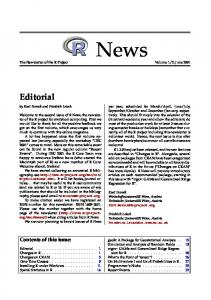
The np Package exper + tenure, data = wage1) wage1.augmented lines(cps71$age, fit.lc, col = "blue") npksum is exceedingly flexible, allowing for leave-one-out sums, weighted sums of matrices, raising the kernel function to different powers, the use of convolution kernels, and so forth. See ?npksum for further details.
12. A parallel implementation Data-driven bandwidth selection methods are, by their nature, computationally burdensome. However, many bandwidth selection methods lend themselves well to parallel computing approaches. High performance computing resources are becoming widely available, and multiple CPU desktop systems have become the norm and will continue to make inroads. When users have a large amount of data, serial bandwidth selection procedures can be infeasible. For this reason, we have developed an MPI-aware version of the np package that uses some of the functionality of the Rmpi package which we have tentatively called the npRmpi package and is available from the authors upon request (the Message Passing Interface (MPI) is an open library specification for parallel computation available for a range of computing platforms). The functionality of np and npRmpi is identical, however, using npRmpi you could take advantage of a cluster computing environment or a multi-core/multi-CPU desktop machine thereby alleviating the computational burden associated with the nonparametric analysis of large datasets. Installation of this package, however, requires knowledge that goes beyond that which even seasoned R users may possess. Having access to local expertise would be necessary for many users therefore this package is not available via CRAN.
13. Summary The np package offers users of R a variety of nonparametric and semiparametric kernel-based methods that are capable of handling the mix of categorical and continuous data typically
30
15
The np Package
●
●
● ●
●
●
●
●
● ● ●
●
●
● ●
●
●
●
● ●
14
● ● ● ●
● ● ●
●
●
● ●
●
●
●
●
● ●
●
●
●
●
● ●
●
●
●
●
● ●
● ●
●
● ● ●
●
●
● ●
● ●
●
●
●
●
●
●
● ●
●
●
●
●
● ● ●
● ● ●
●
●
●
●
●
●
●
● ● ●
●
● ●
●
●
● ●
●
●
●
● ●
●
●
●
●
● ● ●
●
●
●
● ●
●
●
●
●
●
● ●
●
●
●
●
●
●
●
● ●
●
●
●
● ●
● ●
●
●
● ●
●
●
●
●
● ● ●
●
●
● ●
●
● ●
●
●
● ●
●
13
log(wage)
●
●
●
●
●
●
● ●
●
●
● ● ●
●
●
●
●
● ● ●
●
●
●
●
●
●
●
● ●
12
●
●
● ● ●
●
●
● ●
●
●
●
●
●
20
30
40
50
60
Age
Figure 6: A local constant kernel estimator generated with npksum for the cps71 dataset.
encountered by applied researchers. In this article we have described the functionality of the np package via a series of illustrative applications that may be of interest to applied econometricians interested in becoming familiar with these methods. We do not delve into details of the underlying estimators, rather we provide references where appropriate and direct the interested reader to those resources. The help files accompanying many functions found in the np package contain numerous examples which may be of interest to some readers, and we encourage readers to experiment with these examples in addition to those contained herein. Finally, we encourage readers who have successfully implemented new kernel-based methods using the npksum function to send such functions to us so that they can be included in future versions of the np package with appropriate acknowledgment of course.
Acknowledgments We are indebted to Achim Zeileis and to two anonymous referees whose comments and feedback have resulted in numerous improvements to the np package and to the exposition of this article. Racine would like to gratefully acknowledge support from the Natural Sciences and
Tristen Hayfield, Jeffrey S. Racine
31
Engineering Research Council of Canada (http://www.nserc.ca), the Social Sciences and Humanities Research Council of Canada (http://www.sshrc.ca), and the Shared Hierarchical Academic Research Computing Network (http://www.sharcnet.ca).
References Aitchison J, Aitken CGG (1976). “Multivariate Binary Discrimination by the Kernel Method.” Biometrika, 63(3), 413–420. Baiocchi G (2006). “Economic Applications of Nonparametric Methods.” Ph.d. thesis, University of York. Canty A, Ripley BD (2008). boot: Functions and Datasets for Bootstrapping. R package version 1.2-33, URL http://CRAN.R-project.org/package=boot. Gau Q, Liu L, Racine J (forthcoming). “A partially linear kernel estimator for categorical data.” Econometric Reviews. Granger CWJ, Maasoumi E, Racine JS (2004). “A Dependence Metric for Possibly Nonlinear Processes.” Journal of Time Series Analysis, 25(5), 649–669. Hall P, Li Q, Racine JS (2007). “Nonparametric Estimation of Regression Functions in the Presence of Irrelevant Regressors.” The Review of Economics and Statistics, 89, 784–789. Hall P, Racine JS, Li Q (2004). “Cross-Validation and the Estimation of Conditional Probability Densities.” Journal of the American Statistical Association, 99(468), 1015–1026. Hayfield T, Racine JS (2008). “Nonparametric Econometrics: The np Package.” Journal of Statistical Software, 27(5). URL http://www.jstatsoft.org/v27/i05/. Hsiao C, Li Q, Racine JS (2007). “A Consistent Model Specification Test with Mixed Categorical and Continuous Data.” Journal of Econometrics, 140, 802–826. Hurvich CM, Simonoff JS, Tsai CL (1998). “Smoothing Parameter Selection in Nonparametric Regression using an improved Akaike information criterion.” Journal of the Royal Statistical Society Series B, 60, 271–293. Ichimura H (1993). “Semiparametric Least Squares (SLS) and Weighted SLS Estimation of Single-Index Models.” Journal of Econometrics, 58, 71–120. Klein RW, Spady RH (1993). “An Efficient Semiparametric Estimator for Binary Response Models.” Econometrica, 61, 387–421. K¨ unsch HR (1989). “The Jackknife and the Bootstrap for General Stationary Observations.” The Annals of Statistics, 17(3), 1217–1241. Li Q, Maasoumi E, Racine JS (2009). “A Nonparametric Test for Equality of Distributions with Mixed Categorical and Continuous Data.” Journal of Econometrics, 148, 186–200. Li Q, Ouyang D, Racine J (forthcoming). “Categorical Semiparametric Varying-Coefficient Models.” Journal of Applied Econometrics.
32
The np Package
Li Q, Racine J (2008). “Nonparametric Estimation of Conditional CDF and Quantile Functions with Mixed Categorical and Continuous Data.” Journal of Business and Economic Statistics, 26(4), 423–434. Li Q, Racine JS (2003). “Nonparametric Estimation of Distributions with Categorical and Continuous Data.” Journal of Multivariate Analysis, 86, 266–292. Li Q, Racine JS (2004). “Cross-Validated Local Linear Nonparametric Regression.” Statistica Sinica, 14(2), 485–512. Li Q, Racine JS (2007). Nonparametric Econometrics: Theory and Practice. Princeton University Press. Li Q, Racine JS (2010). “Smooth Varying-Coefficient Estimation and Inference for Qualitative and Quantitative Data.” Econometric Theory, 26, 1607–1637. Liu RY (1988). “Bootstrap Procedures Under Some Non I.I.D. Models.” Annals of Statistics, 16, 1696–1708. Maasoumi E, Racine JS (2002). “Entropy and Predictability of Stock Market Returns.” Journal of Econometrics, 107, 291–312. Maasoumi E, Racine JS (2009). “A robust entropy-based test of asymmetry for discrete and continuous processes.” Econometric Reviews, 28, 246–261. Nadaraya EA (1965). “On Nonparametric Estimates of Density Functions and regression curves.” Theory of Applied Probability, 10, 186–190. Ouyang D, Li Q, Racine JS (2006). “Cross-Validation and the Estimation of Probability Distributions with Categorical Data.” Journal of Nonparametric Statistics, 18(1), 69–100. Pagan A, Ullah A (1999). Nonparametric Econometrics. Cambridge University Press, New York. Parzen E (1962). “On Estimation of a Probability Density Function and Mode.” The Annals of Mathematical Statistics, 33, 1065–1076. Politis DN, Romano JP (1994). “Limit Theorems for Weakly Dependent Hilbert Space Valued Random Variables with Applications to the Stationary Bootstrap.” Statistica Sinica, 4, 461–476. R Core Team (2013). R: A Language and Environment for Statistical Computing. R Foundation for Statistical Computing, Vienna, Austria. ISBN 3-900051-07-0, URL http: //www.R-project.org/. Racine JS (1997). “Consistent Significance Testing for Nonparametric Regression.” Journal of Business and Economic Statistics, 15(3), 369–379. Racine JS (2006). “Consistent Specification Testing of Heteroskedastic Parametric Regression Quantile Models with Mixed Data.” Unpublished manuscript, McMaster University. Racine JS, Hart JD, Li Q (2006). “Testing the Significance of Categorical Predictor Variables in Nonparametric Regression Models.” Econometric Reviews, 25, 523–544.
Tristen Hayfield, Jeffrey S. Racine
33
Racine JS, Li Q (2004). “Nonparametric Estimation of Regression Functions with both Categorical and Continuous Data.” Journal of Econometrics, 119(1), 99–130. Racine JS, Li Q, Zhu X (2004). “Kernel Estimation of Multivariate Conditional Distributions.” Annals of Economics and Finance, 5(2), 211–235. Robinson PM (1988). “Root-N Consistent Semiparametric Regression.” Econometrica, 56, 931–954. Rosenblatt M (1956). “Remarks on some Nonparametric Estimates of a Density Function.” The Annals of Mathematical Statistics, 27, 832–837. Wand M, Ripley B (2008). KernSmooth: Functions for Kernel Smoothing. R package version 2.22-22, URL http://CRAN.R-project.org/package=KernSmooth. Watson GS (1964). “Smooth Regression Analysis.” Sankhya, 26:15, 359–372. Wooldridge JM (2003). Introductory Econometrics. Thompson South-Western. Zheng J (1998). “A Consistent Nonparametric Test of Parametric Regression Models Under Conditional Quantile Restrictions.” Econometric Theory, 14, 123–138.
Affiliation: Tristen Hayfield ETH H¨onggerberg Campus Physics Department CH-8093 Z¨ urich, Switzerland E-mail:
[email protected] URL: http://www.exp-astro.phys.ethz.ch/hayfield/ Jeffrey S. Racine Department of Economics McMaster University Hamilton, Ontario, Canada, L8S 4L8 E-mail:
[email protected] URL: http://www.mcmaster.ca/economics/racine/
34
The np Package
Function npcdens npcdensbw
Description Nonparametric Conditional Density Estimation Nonparametric Conditional Density Bandwidth Selection npcdist Nonparametric Conditional Distribution Estimation Parametric Model Specification Test npcmstest npconmode Nonparametric Modal Regression npdeneqtest Nonparametric Test for Equality of Densities Nonparametric Entropy Test for Pairwise Depennpdeptest dence Semiparametric Single Index Model npindex npindexbw npksum npplot npplreg
Semiparametric Single Index Model Parameter and Bandwidth Selection Nonparametric Kernel Sums General Purpose Plotting of Nonparametric Objects Semiparametric Partially Linear Regression
npqreg npreg
Semiparametric Partially Linear Regression Bandwidth Selection Parametric Quantile Regression Model Specification Test Nonparametric Quantile Regression Nonparametric Regression
npregbw
Nonparametric Regression Bandwidth Selection
npscoef npscoefbw
npsigtest
Semiparametric Smooth Coefficient Regression Semiparametric Smooth Coefficient Regression Bandwidth Selection Nonparametric Entropy Test for Serial Nonlinear Dependence Nonparametric Regression Significance Test
npsymtest npudens
Nonparametric Entropy Test for Asymmetry Nonparametric Density Estimation
npudensbw
Nonparametric Density Bandwidth Selection
npudist
Nonparametric Distribution Estimation
npunitest
Nonparametric Entropy Test for Univariate Density Equality
npplregbw npqcmstest
npsdeptest
– Utilities – gradients Extract Gradients se Extract Standard Errors uocquantile Compute Quantiles/Modes for Unordered, Ordered, and Numeric Data
Table 1: np functions.
Reference Hall et al. (2004) Hall et al. (2004) Li and Racine (2008) Hsiao et al. (2007) Li, Maasoumi, and Racine (2009) Maasoumi and Racine (2002) Ichimura (1993), Spady (1993) Ichimura (1993), Spady (1993)
Klein
and
Klein
and
Robinson (1988), Gau et al. (forthcoming) Robinson (1988), Gau et al. (forthcoming) Zheng (1998), Racine (2006) Li and Racine (2008) Racine and Li (2004), Li and Racine (2004) Hurvich, Simonoff, and Tsai (1998), Racine and Li (2004), Li and Racine (2004) Li and Racine (2010) Li and Racine (2010) Granger, Maasoumi, and Racine (2004) Racine (1997), Racine et al. (2006) Maasoumi and Racine (2009) Parzen (1962), Rosenblatt (1956), Li and Racine (2003) Parzen (1962), Rosenblatt (1956), Li and Racine (2003) Parzen (1962), Rosenblatt (1956), Li and Racine (2003) Maasoumi and Racine (2002)