Vol. 120 (2011)
ACTA PHYSICA POLONICA A
No. 4
Optical and Acoustical Methods in Science and Technology
The Numerical Synthesis of a Radar Signal Based on Iterative Method C. Lesnik, A. Kawalec and M. Szugajew∗ Institute of Radioelectronics, Military University of Technology Gen. S. Kaliskiego 2, 00-908 Warsaw, Poland This paper presents the impact of numerical methods used to solve the problem of synthesis of signals modulated in frequency with an autocorrelation function that implements an optimal approximation to a given autocorrelation function. After theoretical introduction an algorithm of frequency modulated signal synthesis is presented. Simulation results made in Matlab are presented in the last section. PACS: 03.50.De
1. Introduction The signal to the interference ratio at the receiver input is a characteristic that has a particular impact on a radar system performance. This is due to the fact that the radar probability of detection of useful signals depends on this parameter. Therefore, one of the parts of a radar receiver is a matched filter which is optimum solution of the problem of filtration in the sense of maximizing the signal-to-noise (SNR) ratio. The signal at the output of such a filter, when the signal on its input is the useful signal (e.g. echo of a single point object), is proportional to the autocorrelation function. The shape of this function determines the accuracy and resolution of distance measurements made with the radar system. The main merit factors of the quality of the autocorrelation function of the transmitted signal are its main lobe width and side lobes level. Therefore, the main problem which a designer of radar systems must face is the optimization of a probing signal waveform in terms of reduction of these parameters. One method of forming the autocorrelation function of the probing signal, and thus the signal at the output of the matched filter, is to change the inner structure of the signal. Signals with nonlinear frequency modulation (NLFM), with appropriately selected frequency modulation function, can have a reduced side lobes level and a higher SNR at the output of the matched filter without use of weighting functions. Thus the signals synthesis task is to determine signal x, that is an element of a set of frequency modulated signals X, on the basis of the set of signals Y having desired property or properties of autocorrelation function. In other words one should synthesize xopt signal which is closest to yopt signal in the meaning of square criterion. The synthesis of optimum signal xopt is equivalent
∗
corresponding author; e-mail:
[email protected]
to determination of shortest distance d(x, y), in sense of square criterion, between the X and Y sets [1], i.e. dmin = min d(x, y) . x∈X
(1)
Square criterion specifies a rule according to which to each pair of functions x and y a distance d(x, y) is assigned to. The distance d(x, y) is often called a function space metric and should not be interpreted as the geometric distance. Signals belonging to this space are governed in terms of energy. 2. Signal synthesis algorithm In this section the proposed algorithm of signal synthesis will be described in detail. The signal synthesis algorithm is presented in Fig. 1. The whole problem of signal synthesis was divided into two parts. First part (first three blocks from Fig. 1) is carried out only once during the initial work of the algorithm and its purpose is to find the form of Eq. (iv) from Fig. 1. The second part of the problem of signal synthesis is solved, by building two separate algorithms (Fig. 1, last two blocks). The second part of the problem of solving the signal synthesis task was divided into two separate steps, algorithms. In the first step a facultative signal x ∈ X is chosen and the best approximation on Y set of signals is determined, this is performed by the main program from Fig. 1. The quality of approximation is characterized by a distance expressed by the following: d(x, Y ) = kx − yk ,
(2)
where k.k — norm of the signal. This distance corresponds to a specific signal y0 : y0 = a(ω)e− j β0x .
(3)
If the signal does not have the desired properties, the signal x is changed (moving inside X set), and the distance d(x, y) is determined again, this task is carried out (693)
694
C. Lesnik, A. Kawalec, M. Szugajew
by iterative program from Fig. 1. Successive distance values should form a decreasing sequence d1 > d2 > d3 > . . . This operation is repeated until the minimum of (2) is achieved. Both algorithms were implemented in Matlab using numerical methods. The main algorithm from Fig. 1 will now be presented in detail.
y˜(ω) = a(ω)e j α(ω) ,
(8)
where A(t) is envelope of signal y(t), Φ(t) is phase function of signal y(t), α(ω) is phase spectrum of signal y˜(ω), a(ω) is amplitude spectrum of signal y˜(ω). The signals x(t) ∈ X differ only in the form of the phase modulation function ϕ(t), with a given envelope a(ω). With given functions a(ω) and B(t) one synthesizes the phase modulation function ϕ(t) (or βx (ω)), which minimizes the distance between the X and Y sets [2]. This means that one must determine the similarity coefficient Z ∞ 1 C(x, Y ) = a(ω)bx (ω) dω = max , (9) 2π −∞ where ¯Z ¯ ¯ ¯ j (ϕ(t)−ωt) ¯ bx (ω) = |˜ x(ω)| = ¯ B(t)e (10) dt¯¯. The optimal frequency modulation function, which maximizes the similarity coefficient (9), shall be determined on the basis of the differential equation 1 2 B 2 (t)dt = a (ωc )dωc . (11) 2π After determining the frequency modulation function ωc (t) from the above equation, in the next step the phase modulation function is determined as Z ϕ(t) = ωc (t)dt . (12)
Fig. 1.
Signal synthesis algorithm.
The task of signal synthesis, and the task of main algorithm, is to synthesize the frequency modulation function ωc (t) that realizes the best approximation to the desired signal y(t). Suppose that the elements of the set of possible signals X are given as T x(t) = B(t)e j ϕ(t) for |t| ≤ , (4) 2 where T is the pulse duration, B(t) is the signal envelope, ϕ(t) is the phase modulation function. The spectrum of the signal x(t): ˜ X(ω) = bx (ω)e− j βx (ω) ,
(5)
where bx (ω) is the amplitude spectrum, βx (ω) is the phase spectrum. In the process of synthesis, it is assumed that the envelope of signal B(t) is set, and the function ϕ(t) is arbitrary. The frequency modulation function is expressed as follows: dϕ(t) . (6) ωc (t) = dt The elements of Y have the following form: y(t) = A(t) e j Φ(t) , and their spectra can be written as
(7)
In order to determine the phase spectrum of signal x(t) one must solve the integral Z T /2 ˜ X(ω) = B(ω) e j (ϕ(t)−ωt) dt. (13) −T /2
Using the method of stationary phase [3] one obtains a solution of the form h πi βx (ω) = − ϕ(t) − ωt0 ± , (14) 4 where t0 is the point of stationary phase. In the next step, from the above equation the phase spectrum βx (ω) should be determined, which is then mapped onto a specified amplitude spectrum a(ω), in order to obtain the signal y(t) closest to the signal x(t) y˜0 (ω) = a(ω)e j βx (ω) .
(15)
The determined spectrum βx (ω) belongs both to the signals xopt (t) and y0 (t). Signal y0 (t) is obtained by taking the inverse Fourier transform from signal y˜0 (ω). At this stage, namely after the determination of the signal xopt (t), the main algorithm ends. The results of the main program are affected by errors. These errors are coming from stationary phase method and numerical methods used in the Matlab program that implements the algorithm. In order to reduce them an iterative method was built and the signal y˜0 (ω) is the input signal for this method.
The Numerical Synthesis of a Radar Signal Based on Iterative Method
695
In the next paragraph the simulation results of both programs, main and iterative, are presented with aspects of additional errors induced by numerical methods. 3. Simulation results As was mentioned in the first paragraph the main and iterative algorithms were implemented in Matlab with extensive use of various numerical methods. The aspects of additional errors induced by these methods to the results of the signal synthesis will be now presented. The goal of the proposed algorithms can be written as: With the given functions a(ω) and B(t) the phase function ϕ(t) (or βx (ω)) of the optimal signal xopt (t) is synthesized. This function minimizes the distance between the sets X and Y . On the basis of the shape of xopt (t) signal, having the optimal phase function ϕ(t), the resulting autocorrelation function Ropt (t) is determined. In order to demonstrate the impact of the numerical methods that were used on the program output, the synthesis of signal with a NLFM having a bell shaped amplitude spectrum, given by p 2/Ω p a(ω) = , −∞ < ω < +∞ (16) 1 + ω 2 /Ω 2 was made. The envelope of the synthesized signal has rectangular shape ( √1 for − T2 ≤ ω ≤ T2 , T B(t) = (17) 0 for |t| > T2 .
Fig. 3. Obtained autocorrelation function of the synthesized signal.
problem that must have been overcome. The solution was the polynomial curve fitting. After applying this numerical method the main algorithm gained more flexibility. From this moment on it can work on not uniformly spaced, sparse data set. Another key aspect of this method is that it does not slow down the process of synthesis as much as one could expect. The approximation is carried out only once, after that only the polynomial coefficients are stored in the system memory. The only problem that had to be solved in order to apply the polynomial curve fitting was the choice of the polynomial degree. For this purpose, a simple experiment in changing the degree of the polynomial and calculating the mean square error, which reflects the accuracy of approximation, was made.
On the basis of the given amplitude spectrum a signal with NLFM function was obtained (Fig. 2).
Fig. 2. Frequency modulation function of the synthesized signal.
The obtained autocorrelation function of the synthesized signal is presented in Fig. 3. As one can see the level of all side lobes is almost constant and does not exceed −40 dB. Those are the best results that authors achieved during the synthesis on the basis of the amplitude spectrum (16). In its first version the main algorithm required on its input uniformly a spaced data set (amplitude spectrum samples) in order to work correctly. Moreover, the data points must have been closely spaced. This was the first
Fig. 4. n = 3.
Polynomial curve fitting of amplitude spectrum
Figure 4 summarizes the results of the polynomial approximation of the data set with a degree 3 polynomial. Figure 5 illustrates how the use of this polynomial affects the outcome of the synthesis. As it can be seen, the final result of the synthesis is much worse than that shown in Fig. 3. This comes from the fact that the input spectrum is subject to substantial error and does not resemble the ideal spectrum shape as shown in Fig. 4. The outcome of the main algorithm (on the basis of which the autocorrelation function from Fig. 5a was
696
C. Lesnik, A. Kawalec, M. Szugajew
drawn) was next sent to the input of the iterative algorithm. This algorithm also needs on its input the amplitude spectrum (Fig. 1). In this case this spectrum is free of errors. Figure 5b shows how the iterative algorithm minimizes the incorrect result of the main algorithm in subsequent iterations. In the course of experiments it was found that a polynomial of 30th degree gives the best results.
as before was made: interpolate the data set with several interpolation methods, and calculate the mean square error to compare the results. The experiment results are illustrated in Fig. 6, where the upper figure shows the results of interpolation of the data set with piecewise cubic Hermite interpolation (pchip) and spline interpolation. As it can be seen, pchip method gives the worst results. On the margins the spectrum is highly distorted, it deviates from the ideal spectrum (black line) most. The spline interpolation (green line) gives much better results. Although the curve deviates from the ideal curve, the nature of the changes is preserved. The superiority of the spline interpolation can be seen in Figs. 5b, c. Figure 5b illustrates the result of synthesis, when the iterative algorithm used piecewise interpolation and Fig. 5c illustrates the result of synthesis when the iterative algorithm used spline interpolation.
Fig. 5. Polynomial curve fitting summary; (a) autocorrelation function of synthesized signal on the output of main algorithm n = 3; (b) amplitude spectra on the exit of selected iterations; (c) autocorrelation function after 30 iterations.
Another problem that arose and had to be solved during the encoding of the iterative algorithm is the fact that the data set (points of the amplitude spectrum) did not cover whole frequency band, as shown in Fig. 6a. By definition, that: Curve fitting: Finding a function (curve) that best fits a set of measured x values and corresponding y values. Interpolating: Estimating the value of yi corresponding to a chosen xi having value between the measured x values. Thus, the objective is not to fit the entire range of data with a single curve, as the case of curve fitting, but rather to use the data to estimate a yi value corresponding to xi . According to above definitions it was decided to solve the second problem by means of interpolation. As in the previous case, there are many methods of interpolation. In order to select the best of them the same experiment
Fig. 6. The interpolation experiment results: (a) comparison of interpolation methods; (b) the autocorrelation function of synthesized signal after the pchip interpolation; (c) the autocorrelation function after the spline interpolation.
As one can see, the autocorrelation function side lobes in Fig. 5b are much higher and are not on equal level. Using spline interpolation gave much better results. Side lobes of autocorrelation are on much lower level and are almost equal. That is why the spline interpolation was chosen as the interpolation scheme used in the signal synthesis algorithm.
The Numerical Synthesis of a Radar Signal Based on Iterative Method
697
4. Conclusion
Acknowledgments
This paper discusses key aspects of the signal synthesis needed for the selection of signals with a desired autocorrelation function to implement for example in the radar technology. The results of previous studies as the theoretical and numerical results confirm the usefulness of the method discussed in the article from the standpoint of the signal optimization. The iterative method reduces the errors induced by the stationary phase method and the errors that are coming from the used numerical methods. The presented method of the signal synthesis is very useful for the cases where the desired autocorrelation function and the subsequent results of the calculations cannot be represented in a strict analytical form. Another key advantage of the presented algorithm is that the used numerical methods allow to find the optimal solution, having at the entrance, only a discrete set of desired signals amplitude spectrum points without any prior knowledge about the signal itself. Another key aspect of this method is that it is tolerant to input errors.
This work was supported by the Polish Ministry of Science and Higher Education from sources for science in the years 2009–2011 under project OR00006909. References [1] A. Kawalec, C. Lesnik, J. Solowicz, E. Sedek, M. Luszczyk, Elektronika 3, 76 (2009) (in Polish). [2] C.E. Cook, M. Bernfeld, Radar Signals: Introduction to Theory and Application, Artech House, Norwood (MA) 1993. [3] D.E. Vakman, R.M. Sedletzkiy, Problems of Synthesis of Radiolocation Signals, Sovietskoye Radio, Moskva 1973 (in Russian).