Transfer and sharing of data between coupled multiphysics phenomena during simulations: the Phenomenon Computational Pattern F. C. G. Santos E. R. de Brito Jr Mechanical Engineering Department Federal University of Pernambuco Recife - PE, Brazil Abstract - Simulation of natural phenomena, such as temperature and air flow distribution inside a room, evolution of material damage due to mechanical and chemical loads, are crucial in the daily life of engineers. This paper presents the Computational Phenomenon Pattern, whose objective is to standardize - through computational abstraction - the complex interactions of coupled natural phenomena in the context of the Finite Element Method. The pattern makes it intuitive and easier the representation of data sharing and dependence between different coupled phenomena when developing simulators based on the Finite Element Method. The pattern models natural phenomena data, the involved processes and their relationships, which are used in a typical simulation process. Keywords: simulation
1
Finite
Element
Method,
Multi-physics
Introduction
Computational Mechanics has had a profound impact on science and technology over the past three decades. The Computational Mechanics software industry generates several billions of dollars per year [1]. However, in many aspects, it applies software engineering development techniques related to the seventies. Computational Mechanics is effective in solving problems that interest society and in providing deeper understanding of natural phenomena. The enormous success of Computational Mechanics resides in its predictive power, making it possible the simulation of complex natural events and the further use of these simulations in the design of engineering systems. This is done through the so called computer modeling: the development of discretized versions of the theories of mechanics, which are amenable to digital computation, together with complex processes of manipulating these digital representations to produce abstractions of the way real systems behave [1]. The Finite Element Method (FEM) has been frequently used in the field of Computational Mechanics, which has come to rely
J. M. A. Barbosa J. M. B. Silva Mechanical Engineering Department Federal University of Pernambuco Recife - PE, Brazil heavily on this technique. Gradually the FEM is becoming the most popular analyzing procedure within various fields of design [2]. In its very essence - in the abstract and computational senses - the FEM comprises the production and assembling of global algebraic systems (discrete behavior laws), which are solved by software components called solvers. Those global algebraic systems are assembled from small matrices and vectors, which are computed based on each finite element (a small portion of the geometry of the problem) and on the definition of the discrete behavior law of each phenomenon. Thus, each phenomenon contributes in its own way to the global algebraic system - data and processes to do so may be different from one phenomenon to other. Therefore, one can consider the main processes of the FEM as those related to the production of small matrices and vectors, which are assembled and used in an articulated form by a specific solution algorithm (solvers). A solution algorithm means one among many ways of performing the desired multi-physics simulation - that is, solving the global algebraic system of equations. The computation of a phenomenon's contribution (matrices and vectors) may depend on (be coupled to) a number of pieces of data from other phenomena. This is the case of multi-physics systems. We can define multi-physics as a qualifier for a set of interacting phenomena, in space and time. Such phenomena are usually of different natures (deformation of solids, heat transfer and electromagnetic fields) and may be defined in different scales of behavior (macro and micro mechanical behavior of materials). Sometimes a multiphysics system is also called a coupled phenomena system. The Phenomenon Pattern represents an abstraction of the collection of commonalities found in the concepts and processes for representing phenomena simulation through FEM. A further objective with such an abstraction is to make the representation of data sharing and dependence
between different phenomena and between phenomena and solvers intuitive and easy. Before proceeding further in the description of the pattern, it is important to acknowledge that the computation of small matrices and vectors at the finite element level depends on a number of choices like, for instance, local order of approximation, definition of shape functions, numerical integration schemes, etc. Although the dealing with all those pieces of data are considered by the Phenomenon Pattern, we will not focus on this aspect, since it is not the more troublesome one. Instead, we will stress the relationship Phenomenon objects may establish with the solver and with each other during the computation of coupled quantities. This work presents a set of results obtained by researchers of PLEXUS Project. The main objective of PLEXUS is the development of simulators for multi-physics and multiscales systems with strong emphasis in reusability, maintainability and adaptability. The general set of methods currently being considered is the one known by the general name of the finite element method. However, strong attempts are being done in the sense of considering architectures, which could be used for other methods as well - for instance, finite volume method [4].
2
Context
In the definition of a simulation problem the user defines the involved natural Phenomena (e.g. fluid flows and heat transfer). The discrete formulation of a phenomenon comprises a set of algebraic equations (either linear or non linear) obtained through the application of a finite element technique to the exact mathematical formulation. The application of such techniques can be described using FEM concepts such as: finite elements, shape functions, discrete weak forms, discrete vector fields, nodal values, couplings, linear solvers, non-linear solvers, error estimation, adaptivity, and time progression schemes [4]. It is assumed that the reader has a basic knowledge about the finite element method. The following levels of procedures can be recognized in the development of simulators using the finite element method: i. The finite element level: a.
Sub-level of the production of matrices and vectors
b.
Sub-level of the post-processing
c.
Sub-level of the error estimation
ii.
The solution level, composed of: a.
Sub-level of the assembling of algebraic systems and its solution;
b.
Sub-level of interactions, which articulate solutions of different algebraic systems;
c.
Sub-level of loops and interactions involving progression in time and adaptation of models and discretizations.
The definition of those levels is important in the sense of software modularizations. But it does not indicate how to deal with separation of concerns for processes and data and how to define abstractions, which could represent the relationships between entities from different levels and, thus, increase the degree of reusability and maintainability of the software. This is not much of a problem when dealing with uncoupled phenomena - and, actually, many researchers have done it - because the algebraic equations of each phenomenon can be solved independently, thus reducing dramatically the degree of complexity mainly at the finite element level. Coupled multi-physics problems make things very complex at both levels, the finite element level and the solution level. For those problems, the abstractions used for uncoupled systems can not be used efficiently anymorein the sense of reusability, adaptability and maintainability. Those abstractions are not fit to adequately represent the data transfer and dependency, which may occur in coupled multi-physics simulations, because there is a strong relation between decisions at one level (solution level) and computations at the other level (finite element level). The reason why this difficulty arises can be further clarified by analyzing the processes at the lowest level, that is, the finite element level. Those processes are related to the computation of small matrices and vectors (at each finite element) and their assembling into large respective matrices and vectors for each phenomenon. The elemental matrices and vectors may be coupled with other phenomena, meaning that the computations of those quantities need pieces of information from other phenomena. Those pieces of information are defined at the solution level. Changing solution algorithms may produce widely spread changes across both levels. Furthermore, more than one phenomenon can be defined in the same geometry, making them coupled in a another sense (sharing geometric data and meshes, for instance). Therefore, coupled multi-physics problems produce many dependencies and relationships, which should be appropriately considered. Those aspects explains why
software development cost for multi-physics systems became a strong concern for scientists and engineers, who wanted to study them.
should stored in the PhenNodes. Further on, each PhenNode, say the jthone, to have an indexed set
The difficulty just described generates a problem that can be phrased as: What abstraction can adequately represent and encapsulate the information, relationships and processes pertaining to the finite element level, which are concerned to the numerical modeling of a natural phenomenon, and also satisfying the requirements imposed by a large set of solution algorithms in the context of the finite element method and coupled multiphysics problems ? The next sections present a solution to this problem.
3
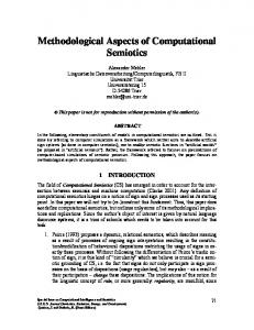
Figure 1. Geometry Graph
The Phenomenon Pattern
For the sake of simplicity of explanation, as we have written before, Phenomenon is considered as a machine for computing small matrices and vectors and assembling them into given large matrices and vectors. The computation of those small matrices and vectors is performed on each finite element of a mesh. The Phenomenon Pattern (called Phenomenon from now on) can be viewed as a container with two acyclic graphs: the PhenGraph and the GeomGraph (see Figs.(1), (2), (3) and (4)). Both of them has exactly the same structure as graphs, but the pieces of data stored in each GraphNode are different. In GeomGraph, the geometry data is stored in the Brep structure (boundary representation). That is, from the root of the graph to the leaves one goes from the higher dimension geometric entities (volumes, for instance) to lower dimension ones (points). On the other hand, in PhenGraph one finds the set of procedures, which are to be computed on the respective geometric entity. Thus, from the root of PhenGraph to its leaves, each GraphNode contains a set of procedures to be computed on the geometric entities of higher dimension down to the lower dimension ones, respectively. Since geometry can be shared with other phenomena, it is important to have such a separation between phenomena and geometry. Each GraphNode from PhenGraph (PhenNode) knows its respective GraphNode from the GeomGraph (GeomNode) and thus has access to its data. Therefore PhenGraph knows GeomGraph but the converse is not true. Phenomenon also contains an indexed set of quantities Q = {Qi}i=1..n (see QTable in Fig. (4), which represents the set of all quantities (small vectors and matrices) that it is able of computing and assembling into given structures (large matrices and vectors). Here n is the total number of quantities the current Phenomenon can compute and assemble. Some of those quantities are computed on the highest dimension geometric entity and others. are computed on lower dimension ones. Then the procedures responsible for the actual computation of those quantities
Figure 2. Phenomenon Graph qj = {Qjk}k=1..nj ⊂ Q (see qTable in Fig. (4), which represents all quantities the jth PhenNode can compute. Each PhenNode needs some pieces of data in order to be able of computing a certain quantity. Those pieces of data are the following: i. General Data (it serves all quantities): a.
GeomMesh: it is the mesh of the geometry. It is a data structure, which contains all geometric finite elements (for instance, triangles, quadrilaterals, tretrahedra, hexagons, etc; it depends on geometric dimension and mesh generation methods used to obtain it). It belongs to its respective GeomNode.
b. PhenMesh: its is the mesh of the phenomenon. It is a data structure, which contains information about the approximation of the phenomenon's vector field on each geometric finite element (for instance, the order of a polynomial approximation). It is strongly related to the respective GeomMesh. ii. Specific Data (it is specific to a certain quantity) for a quantity Qjk:
Figure 3. Phenomenon-Geometry relationship
o
The root of its PhenGraph has only the quantities needed for the transfer of data.
o
Each quantity cited above is coupled to the respective PhenNode of the coupled phenomenon.
o
Each quantity to be computed need only one coupled state - the state to be transferred.
o
The PhenMesh from the coupled phenomenon is also needed, in order to obtain values of the coupled vector field in any desired point.
o
Finally, there is a need for a search structure in order to find the finite element in the mesh of the coupled phenomenon, which contains a given point. This is important in order to perform integration procedures in one mesh using data from the other.
Now we come to the problem where data needed by procedures in a lower level (computation of quantities on each finite element) is defined at a higher level (the owner of Phenomenon objects). Before going directly to this point, it is better to explain how Phenomenon objects are used.
a.
CoupledPhenNodesjk = { Cjks }s=1..njk: it is the set of PhenNodes pertaining to other phenomena. They are used in order to obtain data from coupled phenomena, which are essential for the computation of Qjk.
Phenomenon classes are supposed to be strongly reusable. They are very detailed pieces of software and contain information, which can be used in many different contexts and geometries. In order to achieve that state we should allow the definition of the coupled states from a coupled phenomenon to be done dynamically at run time (see item (ii).b above). That definition depends on the solution algorithms used in the simulation. Here, the simulator is considered as a pattern [3], [5], [9], which is - simply speaking - a workflow in the form of a tree divided into four layers (see levels of procedures defined in section (2)):
b.
CoupledStatesjks = { Sjksr }r=1..njks: it is the set of states, which should be retrieved from the CoupledPhenNode Cjks. Those states usually represent discrete vector fields.
i. Kernel: set of procedures related to algorithmic structures for the control of loops and interactions involving progression in time and adaptation models and discretizations;
Obs: It should be noted that the use (by a certain phenomenon) of a vector field from other phenomenon raises a number of issues. The main issue is the possibility that both GeomMeshes may be different. In this work we do not treat this important problem in detail. What we should say is that we usually build Phenomenon classes, which are specially tailored for the task of transferring data from one mesh to the other. Such a Phenomenon has the following characteristics:
ii. Block: set of procedures related to the articulation of solutions of different algebraic systems;
Figure 4. Phenomenon Diagram
o
It shares the Phenomenon.
GeomGraph
with
the
coupler
iii. Group: set of procedures related to the assembling and solution of algebraic systems, together with the execution of diverse operations with matrices and vectors. iv. Phenomenon: encapsulates the set of procedures related to the production of small matrices and vectors and to their assembling in given larger data structures. It also performs other computations related to post-processing and error estimation.
quantities are to be used and, for each one of them, what are their coupled states)
Figure 5. Simulator Diagram
Therefore the Group level is the level where definitions about the coupled states take place and are conveyed to each Phenomenon object during a demand for the computation of a certain quantity. The coding of the software components for a Group class needs previous knowledge about the set of indexed data structures from all other Group classes. Because of that feature, a Group class is much less reusable than the classes from the other levels. Whenever a solution algorithm is changed, many Group classes may need to be eliminated from the simulators. However, all Phenomenon classes should be implemented in such a way that no modification at all will be needed. Some minor reprogramming of Block and Kernel procedures may still be needed, but their coding as nodes of a workflow will accommodate that without much work. Now we are in a position to describe in a more detailed fashion the usage of a Phenomenon (call it P) object by its owner, that is, a Group object (call it G): i. G is asked (by its Block) to compute a certain quantity Qg. ii. G retrieves from one of its tables the references to all Phenomenon objects, which contribute to Qg. P is one of them.
Figure 6. Group Diagram The simulation starts with the execution of the root of the Kernel, which uses services provided by a set of Blocks, which in turn uses services from a set of Groups. Each Group owns a set of {Phenomenon objects, which are used to perform the computation of small matrices and vectors, assembling them into given (by its Group) large data structures. The intention of this work is not going too far in the explanation of the details of the interactions between objects across the levels of the Simulator Pattern (see Fig. (5)). Before we proceed further with the description of the lowest level - represented by the Phenomenon Pattern - we need some pieces of information about the structure of Group classes (see Fig. (6)):
iii. G retrieves from another table a set of data for each contributing Phenomenon object. This set of data for the ith-object contains information such as: (I) a set qti = { qij }j=1..ni, containing all quantities from the ithPhenomenon, which contributes to form Qg; (II) for each qij, a set CSij = { Sijk }k=1..nij, containing the coupled states to be used in its computation - the order in which those states are given is important, since they may be from different phenomena; (III) a reference to a data structure (say Kg) where the quantity should be assembled. iv. Suppose, now, that P is given a demand to compute a certain quantity Qr, together with a set of indexes for the coupled states, say CSpr = { Sprk }k=1..npr and a reference to Kg.
i. It has a set of indexed data structures (see DataStructures in Fig. (6)), which can be shared upon demand by its own Phenomenon objects.
v. Then, P transfer the demand to its PhenGraph, which in turn send it to its root (say R).
ii. It has a set of tables, which can be dynamically programmed, containing information about the computation of matrices and vectors; the Phenomenon objects, which contribute to them and how they should do it (that is, which Phenomenon
vi. R checks if it is able of computing the desired quantity. If so, it sends the demand to one of its objects (say W), which is responsible for the computation and assembling of Qr. R sends, together with the data already defined, a set of references, say
CG, to the respective PhenNodes of the PhenGraphs of the coupled Phenomenon objects. vii. W retrieves the set of coupled PhenMeshs (say, CPM) and the respective set of discrete coupled states (say Cs) from the respective set of coupled PhenNodes. This is done by sending a request for the states contained in CSpr to the respective PhenNodes contained in CG. Each coupled PhenNode from CG is able of asking its owner Group for the desired states and sending them back to W. viii. W traverse the PhenMesh (given by R) together with the coupled ones (coupled PhenMeshes contained in CPM) and is able of computing, for each finite element, the quantity Qr - using the coupled discrete states (contained in VF) - and of assembling them into Kg. ix. If R is not able of computing the desired quantity, or if it has already computed it, it will transfer the demand recursively to its children PhenNodes together with the same data it received. The process goes on recursively, until there are no children GraphNodes to be reached.
Phenomenon objects and solution algorithms. An important consequence was that all information and procedures, which are very specific of a solution algorithm (less reusable) are encapsulated in the Group level, while all information and procedures, which are strongly reusable are encapsulated in the Phenomenon level. Experiences with prototypes have shown a tremendous improvement in: (i) the time spent in the development of simulators; (ii) the reusability of software components, opening the way for the building of repositories; (iii) the correctness of software components. References of previous and related work can be found in [5]-[10].
5
References
[1] Committee on Theoretical and Applied Mechanics, Research Directions in Computation al Mechanics. A report of the United States Association for Computational Mechanics, 2000. Available at http://www.usacm.org/org\_cm.htm, accessed on 10/01/2004. [2] Viceconti, M., Replication of Numerical Studies. Personal Communication, posted at
[email protected]. Sent on: March 27, 2002 3:03 pm Subject: BIOMCH-L: BioNet controversial topic no. 5.
Obs: Note that, in the description of the computation of Qr by R, we have considered that all PhenMesh objects (that given by R and the coupled ones contained in CPM) share the same GeomMesh object. Therefore they could be traversed at the same time.
[3] Santos, F.C.G., Lencastre, M., Vieira, M. GIGPattern. The Third Latin American Conference on Pattern Languages of Programming, Pernambuco, Brazil, 2003.
4
[4] Lencastre, M., "Conceptualisation of an Environment for the Development of FEM Simulators", Ph.D. thesis, Centro de Informática, Universidade Federal de Pernambuco, Brazil, 2004.
Conclusions
We have presented a pattern called Phenomenon in order to cope with the difficulties found in the development of simulators for coupled multi-physics problems. It was identified that the solution algorithms employed by simulators provide data at a higher level, which determines many procedures at a lower level. Thus, small changes in the solution algorithm could generate the need for widespread changes along the simulator software, implying in strong reprogramming. A separation of concerns was important to identify that the simulator could be divided into four well-defined hierarchical levels. The part of a solution algorithm, where pieces of data to be used at a lower level are generated, was concentrated at a level called the Group level. The part, at a lower level, where those pieces of data are used was identified as the Phenomenon level. An abstraction for the computational representation of the Phenomenon level was described as a pattern. It was shown that the Phenomenon pattern represents adequately all data pertaining to the discrete behavior laws of a phenomenon (computation of small matrices and vectors), together with the sharing and transfer of data between Phenomenon objects and between
[5] Lencastre, M.; Santos, F., "An Approach for FEM Simulator Development"; Journal of Computational Computational and Applied Mathematics, Vol. 185, issue 2, 2006. [6] Lencastre, M.; Santos, F.; Araújo, J., "A Process Model for FEM Simulation Support Development. Proceedings of the Summer Computer Simulation Conference (SCSC 02), San Diego, California, 2002. [7] Lencastre, M.; Santos, F.; Rodrigues, I., "FEM Simulator based on Skeletons for Coupled Phenomena". Proceedings of the 2nd Latin American Conference on Pattern Languages of Programming (SugarLoafPLoP'2002 Conference), pp.35-48, Brazil, 2002. [8] Lencastre, M.; Santos, F.; Rodrigues I., "FEM Simulation Environment for Coupled Multi-physics Phenomena", - Simulation and Planning In High Autonomy Systems, AIS2002; Theme: Towards
Component-Based Modelling and Simulation. pp. 259266. A publication of the Society for Modelling and Simulation International, Portugal, 2002. [9] Lencastre, M.; Santos F.; Vieira, M., "Workflow for Simulators based on Finite Element Method". Proceedings of the International Conference on Computational Science (ICCS 2003), Melbourne, Australia and Saint Petersburg, Russia. 1(2), pp. 555-565, Springer Verlag, 2003. [10] Lencastre, M.; Santos, F.; Vieira, M., "GIG-Pattern". Proceedings of the 3rd Latin American Conference on Pattern Languages of Programming (SugarLoafPLoP'2003), pp. 293-307, Pernambuco, Brazil, 2003.