The quantum transition state wavepacket method - Semantic Scholar

Faraday Discuss., 1998, 110, 105È118

The quantum transition state wavepacket method John C. Light and Dong Hui Zhang¤ Department of Chemistry and T he James Franck Institute, T he University of Chicago, Chicago, IL 60637, USA

The accurate calculation of thermal rate constants for reactions in the gas phase often requires both accurate potential energy surfaces (PESs) and the use of quantum mechanics, particularly in the case of light atom (H) transfers in reactions with activation energy barriers between reactants and products. The thermal rate constant k(T ) can be calculated directly or as a thermal average over the cumulative reaction probability N(E). Both k(T ) and N(E) can be calculated exactly and directly in terms of Ñux formulations Ðrst presented by Miller et al. In this paper we review the recent reformulation of the calculation of N(E) in terms of the time evolution of transition state wavepackets (TSWPs), which then provides a very e†ective method for reactions with activation energy barriers. This method requires a single time propagation for each TSWP contributing to the desired thermal rate constant from which the required contributions to N(E) for all E can be obtained. We then apply this to the calculation of N(E) and k(T ) for the interesting four atom reaction H (D ) ] CN ] HCN(DCN) ] H(D). The 2 at the linear CNHH conÐguration. system has a metastable well in the2 PES The results and a discussion of the inÑuence of this secondary TS well are presented.

1 Introduction The calculation of thermal rate constants of chemical reactions has long been an important goal of theoretical chemical physicists. For a large class of reactions the reaction rate constants are dominated by the energy required to pass over a barrier on the potential energy surface (PES) leading (approximately) to the Arrhenius form of the rate constants. Classical transition state theory (TST)1,2 and further developments of variational TSTs3h9 provide in many cases excellent approximations to thermal rate constants for heavier systems for which the PES is known with reasonable accuracy. However, the dynamical approximations in such TST calculations make it desirable to have a quantum formulation that is both exact and practical. Such calculations will require accurate knowledge of the PES for the full system, at least in the regions of the potential energy barriers separating reactants and products. In addition, the dynamics must be simulated adequately ; if light atom transfers are involved in the reactions, the use of quantum dynamics, which includes both discrete energy level e†ects and quantum tunneling, is highly desirable. Reaction rate constants can be calculated exactly from thermal averages of exact quantum state-to-state reaction probabilities, i.e. from the S-matrices obtained from full solutions to the SchroŽdinger equation at each energy. For reactions with barriers and with relatively sparse reactant and product quantum states, the full S-matrix can be calculated. Alternatively the time dependent SchroŽdinger equation can be solved for ¤ Present address : Department of Computational Science, National University of Singapore, Singapore 119260. 105

106

Quantum transition state wavepacket method

each initial state to obtain the reaction probability as a function of energy from that state. Substantial improvements in the methods used in such initial state selected wavepacket approaches (ISSWP) now permit four atom systems to be solved exactly.10h15 However, for reactions with a relatively dense distribution of reactant and product states at the energies of interest, the number of energetically open states contributing to the rate constant will be very large. In these cases, the full S-matrices or even the initial state selected reaction probabilities may be very difficult to calculate. In addition, the full S-matrices contain much information on state-to-state probabilities that is averaged to obtain the rate constants. If there is a well deÐned transition state region with an activation energy barrier, it will be much more efficient to attack the calculation of the rate constant directly or via the direct calculation of such averaged quantities as the cumulative reaction probability, N(E). In our discussions below we focus on reactions with activation energies for which transition state type theories are most appropriate. The quantum methods discussed are exact for all types of reactions, but their efficiency is greatest for reactions with barriers. Approaches to the direct quantum calculation of k(T ) and N(E) were formulated some time ago in very important papers by Miller and co-workers.16,17 In these formulations dividing surface(s) between reactants and products can be deÐned as in TST. However, the rate constants or reaction probabilities are given as traces of quantum mechanical (Ñux) operators. These were discussed by Miller at a Faraday Discussion meeting more than ten years ago,18 and have been developed and used in a number of applications since that time.19h27 The original formulations were quite general permitting the desired rate information to be obtained in a number of exact and formally equivalent ways. The choice between formally equivalent approaches was not obvious, and there have been a variety of actual computational approaches developed with the basic aims of providing rigorous and efficient methods to determine the speciÐc dynamical information of interest. Ideally there should be a small number of intuitive and efficient methods, each tailored for the speciÐc system information desired. SpeciÐc methods using the formal deÐnitions of the thermal rate constants, k(T ), have been developed to calculate it directly. Other approaches can determine the cumulative reaction probability, N(E), from which k(T ) can be generated by a Boltzmann average. Yet other approaches can yield more detailed information about reaction from a speciÐed initial state or to a speciÐed Ðnal state, by varying the position of the dividing surface(s). The Ðrst calculation of thermal rate constants by these methods for a “ real Ï system, i.e. a three-dimensional (3-D) calculation of the reaction of a triatomic system on a realistic surface was that of Park and Light23 for, naturally, the hydrogen exchange reaction. This was, in a sense, a “ brute force Ï calculation in which the 3-D Hamiltonian was diagonalized on an L 2 basis. The trace was carried out on the basis of the thermal Ñux operator, determined by Lanczos reduction. The diagonalization permitted the rate constants to be calculated analytically at di†erent temperatures as the time integral of the ÑuxÈÑux correlation function. The fact that the Ñux operator is of low rank22 was utilized to simplify the evaluation of the trace of the correlation function. The validity of this approach was veriÐed by Day and Truhlar28 and applied by these authors to the O ] HD reactions.29 As a general method, however, the calculation had several Ñaws : the diagonalization of HŒ becomes prohibitive for larger systems, and, since no absorbing potential was used, accurate results were limited to low temperatures where the e†ects of reÑections from the grid boundaries could be minimized. The obvious utility of absorbing boundary conditions (optical potentials), developed by Neuhauser and Baer28c in removing the e†ect of grid boundaries and permitting the convergence of the time integral of the correlation functions was demonstrated by Brown and Light.25 More recently a number of improved approaches have been developed. The “ transition state probability operator Ï approach of Manthe and co-workers29h31 for the

J. C. L ight and D. H. Zhang

107

determination of N(E) is elegant. The eigenvalues of this operator are probabilities of reaction from each “ transition state Ï, and can be obtained by iterative procedures. This approach requires the use of optical potentials, absorbing potentials are also utilized in all subsequent approaches. The advantages of the probability operator approach are that it is variational and relatively few eigenvalues are required [if the dividing transition state surface (TSS) is well placed at the top of an activation energy barrier]. The disadvantages are that the eigenvalues [essentially of the Green operator, (H [ E [ ie)~1] are not easy to extract by iterative methods and that they must be determined again at each energy. At each energy the number of eigenvalues required is basically the number of transition states contributing to the reaction at that energy. Two other approaches to the direct calculation of rate constants,26,32,33 following the approach proposed by Park and Light,22 are based on the evaluation of the eigenvectors and eigenvalues of the thermal Ñux operator via Lanczos reduction and propagation of these wavepackets. The use of optical potentials makes short time propagations adequate. However, the propagations must be repeated at each temperature at which k(T ) is desired. These approaches have been applied to several important reactions including Cl ] H ] HCl ] H.34 Manthe and co-workers have combined 2 this approach with an approximate multi-conÐguration time dependent Hartree (MCTDH) propagation that is applicable to larger systems.35,36 Our TSWP method37 di†ers from the above in that the cumulative reaction probabilities at all energies desired are evaluated from a single propagation of each TSWP forward and backward in time, followed by the appropriate Fourier transforms. The N(E)s so obtained can then be thermally averaged to produce the thermal rate constants at all desired temperatures. This has the advantages that only TSWPs in the energy range of interest are required ; the Fourier transforms at each E must be accumulated only on a dividing (TS) surface ; and only one propagation (in ] t and [ t) is required per transition state. The TSWP approach has been successfully applied to calculate N(E) for J \ 038 and recently N(E) (summed over all J)39 for the prototype four atom reaction H ] OH ] H O ] H, which provided the Ðrst fairly accurate theoretical rate con2 a four atom2 reaction. stant for In the following we review the formulation of the TSWP theory and discuss the application to a difficult reaction of interest, the H (D ) ] CN reaction. Since the PES 2 2 conÐguration and a metastable of this system has a transition state in the HwHwCwN well in the CwNwHwH conÐguration, it is not a simple transition state problem. The location of the dividing surface (the transition state) and the convergence of the cumulative reaction probability with respect to the number of transition states included illustrate the difficulties encountered when reactions with “ odd Ï PESs are considered.

2 Theory 2.1 TSWP approach The TSWP approach is similar to the regular time-dependent ISSWP approach to reactive scattering40,41 except for the initial wavepacket construction. In the ISSWP approach, the initial wavepacket is usually a direct product of a gaussian wavepacket for the translational motion located in the reactant asymptotic region and a speciÐc (N [ 1 dimensional) internal state for reactants. In the TSWP approach we Ðrst choose a dividing surface S separating the products from reactants preferably located to minimize the value of the 1density-of-states for the energy region considered. Then initial TSWPs are constructed as the direct products of the (N [ 1 dimensional) Hamiltonian eigenstates on the surface H o/T\e o/ T S i i i

(1)

108

Quantum transition state wavepacket method

and the Ñux operator eigenstate, o ] T with positive eigenvalue j. F o ]T \ j o ]T

(2)

Thus we have o /`T \ o / T o ]T (3) i i The cumulative reaction probability, N(E), from the TSWP approach was derived simply from the formulation for N(E) given by Miller and co-workers,17 N(E) \ 2p2tr[d(E [ H)F d(E [ H)F ], (4) 2 1 where F and F are the quantum Ñux operators at dividing surfaces S and S between 1 2 1 2 reactants and products. The surfaces can be identical, and, for calculation of N(E) only, would normally both be the transition state surface. Here the Ñux operator F is deÐned as F\

1 [d(q [ q )pü ] pü d(q [ q )] 0 q q 0 2k

(5)

where k is the reduced mass, q is the coordinate normal to the dividing surface located at q \ q , which separates products from reactants, and pü is the momentum operator 0 to the coordinate q. In evaluating the trace, we take q advantage of the fact that conjugate the Ñux operator has only two non-zero eigenvalues for one-dimension,21,22,42 ^j with eigenfunctions that are complex conjugates of each other o ]T \ o [T*. We then evaluate the trace in eqn. (4) efficiently in a direct product basis of the Ñux operator eigenstates, which are highly localized near the dividing surface, and the eigenstates of the (N [ 1 dimensional) Hamiltonian on the dividing surface, the transition states. The microcanonical density operator, d(E [ H), will eliminate contributions to N(E) from transition states with internal energy much higher than the total energy, E, thus limiting the number of transition states that must be considered. (Owing to tunneling, of course, the internal states with energy somewhat greater than E can contribute to the cumulative reaction probability.) Thus by choosing a dividing surface with the lowest density of internal states, we can minimize the number of transition states required to converge N(E). Since N(E) in eqn. (4) is represented in terms of d function operators, the evaluation is most efficiently carried out utilizing the Fourier transform identity between the energy and time domains. After constructing the initial wavepackets, we propagated them in time, as in the ISSWP approach. The components of the TSWPs at energy E, o t T, are calculated on the second dividi ing surface (at x \ x ) as 0 `= ei(E~H)tdt o /`T. (6) o t (E)T \ Jj i i ~= o /`T \ o / T o ]T with F o ]T \ j o ]T and H o / T \ e o / T (7) i i S1 i i i The cumulative reaction probability N(E) can be computed as

P

1 (8) N(E) \ ; N (E) \ ; St o F o t T \ ; Im[St o t@T] o i i 2 i i i q/q0 k i i i where the o t@T are the derivatives of o t T with respect to q, the coordinate normal to the i surface evaluated on the surface S (q \i q ). Here q can be any coordinate as long as the 2 0from reactants. surface of F , q \ q divides the products 2 0 There are several points to note concerning this compact formulation. First, since the Ñux operator F exists only at the surface S , the Fourier transform of t and its deriv2 2 i

J. C. L ight and D. H. Zhang

109

ative are required only on that surface, not throughout space. If the surface for F is 2 placed in an asymptotic region, then the Ñux can be projected onto the asymptotic internal states of the reactants (or products) to obtain the cumulative reaction probabilities (and rate constants) from each initial state, i.e. the information obtained from the ISSWP approach. For a single initial state, the ISSWP is to be preferred since only one propagation is required. However, when information for many initial states is desired, and there is a barrier to reaction, then the TSWP approach will converge with many fewer wavepacket propagations. A perhaps surprising point is that the N (E) above, which are the contributions to N(E) from each TSWP are not probabilities, ii.e. N (E) can be negative at some energies i amounts). However, N(E) itself is a and greater than one at others (usually by very small cumulative probability, always greater than zero. Finally, since the TSWPs are determined by the position of the dividing surface S the convergence and behaviour of N (E) 1 i vary with the surface. Placement of S in the “ traditional Ï transition state region seems 1 to yield the most rapid convergence with respect to the number of wavepackets required and also seems to produce N values that are “ almost Ï probabilities. We shall see in the i application below that because some “ transition state Ï wavepackets for the HHCN reaction start out in the HHNC conÐguration, the contributions of these wavepackets are zero at low energies, but oscillate with E at higher energies, and do not behave like probabilities.

3 Applications to the H (D ) + CN reaction 2 2

In this section, we show the results of the application of the TSWP approach to the H (D ) ] CN reaction. These two reactions have been the subject of active theoretical 2 experimental 2 and research43h51 because of their practical importance in combustion and atmospheric chemistry. In particular, a new and much improved global PES for the reaction has recently been reported by ter Horst, Schatz and Harding (denoted TSH3).46 Quasiclassical trajectory calculations,48 a reduced dimensionality quantum scattering calculation,47 as well as a recent full dimensional ISSWP calculation49 have been carried out for these reactions on the TSH3 PES. It is found that the thermal rate constant approximated by the rate constant for the ground initial state from the ISSWP approach49 is signiÐcantly smaller than the experimental values in the low temperature region for the H ] CN reaction. Since the number of open rotational channels for this reaction is huge 2even at quite modest translational energy, owing to the tiny rotational constant of CN, it is obviously not feasible to use the ISSWP approach to obtain the rotationally averaged thermal rate constant. On the other hand, reactions such as this, which have a barrier and therefore a much lower density of states in the transition state region than the asymptotic region, are ideal for the TSWP approach.37 We have used this approach to calculate the exact N(E) (J \ 0) on the TSH3 PES, from which the rate constants were computed by using the energy shifting approximation. 3.1 The Hamiltonian and numerical parameters The Hamiltonian for the diatomÈdiatom system in mass-scaled Jacobi coordinates can be written as38,52

A

B

L2 j2 1 3 ] i ] V (s , s , s , h , h , /) (9) ; [ 1 2 3 1 2 Ls2 s2 2k i i i/1 where j and j are the rotational angular momenta for H (D ) and CN, which are then 3 j . In the body-Ðxed frame the orbital angular 2 2 momentum, j , is repcoupled2 to form 23 resented as (J [ j )2, where J is the total angular momentum. In eqn. (9), 1k is the 23 H\

110

Quantum transition state wavepacket method

reduced mass of the system, k \ (M M M )1@3 1 2 3 with M (i \ 1È3) being the reduced masses for the system, H (D ) and CN, i.e. i 2 2 (m ] m )(m ] m ) H C N , M \ H 1 m ]m ]m ]m H H C N m m M \ H H , 2 m ]m H H m m M \ C N . 3 m ]m C N The mass-scaled coordinates s are deÐned as i M s2 \ i R2 i k i

(10)

(11)

where R (i \ 1È3) are the intermolecular distance between the centers of mass of H and 2 CN, andi the bond lengths for H (D ) and CN, respectively. 2 2 Now we deÐne two new “ reaction coordinate Ï variables q and q by translating and 1 2 rotating the s and s axes,37,53 1 2 q cos s sin s s [ s0 1 \ 1 1 . (12) q [sin s cos s s [ s0 2 2 2 It can be seen from this equation that we Ðrst move the origins of the (s , s ) coordinates 1 2 q and q to (s0, s0), then we rotate these two axes by the angle s. The new coordinates, 1 2 1 2Ï can now be deÐned as the “ reaction coordinate Ï and the “ symmetric stretch coordinate for the collinear HwHw(CN) transition state. The Hamiltonian in eqn. (9) can be written in term of q (i \ 1, 2) and s as i 3 2 L2 L2 2 j2 j2 1 i [; [ ]; ] 3 ]V (13) H\ Lq2 Ls2 s (q , q , s0, s0)2 s2 2k 1 i 3 1 i 1 2 1 2 3 By choosing the dividing surface S at q \ 0, we can calculate the “ internal Ï tran1 sition states for the other Ðve degrees 1of freedom by solving for the eigenstates of the 5-D Hamiltonian obtained by setting q \ 0 in eqn. (13). After constructing the initial 1 wavepackets in (q , q , s , h , h , /) coordinates, we transfer them to the (s , s , s , h , 1 2 3 1 2 1 2 3 The 1 h , /) coordinates, and propagate them as in the regular wavepacket approach. 2 calculation of the bound states in 5-D has been presented in detail elsewhere,54 and the propagation of the 6-D wavepacket in the diatomÈdiatom coordinates has also been shown ;12 thus we will not present them again here. The parameters used in the current study are based on those employed in the initial state selected total reaction probability calculation carried out recently by Zhu et al.49 We used a total number of 55 sine functions (among them 21 for the interaction region) for the translational coordinate s in a range of [3.5, 11.5]a . The number of vibrational 1 CN is 2 or 3 depending 0 on whether CN is vibrabasis functions used for the reagent tionally excited. A total of 19 and 22 vibrational functions are employed for s in the 2 basis, range of [0.3, 2.5]a for the reagents H and D , respectively. For the rotational 0 2 2 we used j \ 41 (for CN), j \ 12 for H and j \ 16 for D . The values of s0, s0 3max 2maxstate surface 2were carefully 2max 2 and s that deÐne the transition chosen 2to be 5.1, 0.8 and147¡ for H ] CN, and 5.5, 0.8 and 48¡ for D ] CN, to minimize the density-of-states on the 2 2

AB A

A

BA

B

B

J. C. L ight and D. H. Zhang

111

dividing surface. We propagated the TSWPs for 9000 au for the H ] CN reaction, and 2 10 500 au for the D ] CN reaction. 2 In addition to the separation of even and odd parities, which are related to the wave function symmetry with respect to torsion angle / \ 055 for the total angular momentum J \ 0, the even and odd rotation states of H (D ) can also be separated. In the 2 2 present study, we only calculated the N(E) for the even rotation of H . Based on the fact 2 that the transition state on the PES is quite rigid, we approximated the N(E) for the odd rotation of H (D ) by that for the even rotation. 2 2 For the H ] CN reaction, we propagated 60 wavepackets (40 for even parity, 20 for odd parity) to2 converge the N(E) for energies up to 0.5 eV with respect to the ground rovibrational states of reagents. For the D ] CN reaction, we propagated 45 wave2 packets (30 for even parity, 15 for odd parity) to converge the N(E) for energies up to 0.4 eV. 3.2 The cumulative reaction probability, N(E) (J = 0) We Ðrst show in Fig. 1 the number of open states of even parity as a function of energy in the asymptotic region and on the dividing surface S for the H ] CN reaction. Very 2 obviously and importantly, the number of open states1 on S is much smaller than the 1 number open in the asymptotic region. For E \ 0.4 eV, for example, the ratio between these is about 16. Thus for this reaction the TSWP should require many fewer wavepacket propagations in order to calculate N(E) than the ISSWP approach. Fig. 2 shows the contributions of N (E) of di†erent transition states to N(E) (i \ 1È5, i can be seen from the Ðgure, the N (E) for the 10, 15, 20, 25, 30, 35 for even parity). As i Ðrst few states rise very quickly from 0 to about 1 in about 0.1 eV energy interval, then slightly decrease as the energy increases further. This rise in N (E) is signiÐcantly faster than that for the H ] OH reaction shown in Fig. 5 in ref. 38.i This probably indicates that there is much 2less tunneling in the H ] CN reaction. Also we can see that the 2 transition states are negligible for energy contributions to N(E) for the highly excited lower than 0.25 eV. The contributions to N(E) in that energy region almost all come from the Ðrst 4È5 transition states. For energy up to 0.5 eV, the Ðrst 40 wavepackets have already given very well converged N(E). Among the N (E) shown in the Ðgure, i however, we can see the “ non-probability Ï nature of N (E) ; some have values slightly i

Fig. 1 Number of open states as a function of total energy on transition state dividing surface and in asymptotic region divided by 10 for the H (even rotation) ] CN reaction in even parity 2

112

Quantum transition state wavepacket method

Fig. 2 Some N (E)s (i \ 1È5, 10, 15, 20, 25, 30, 35, 40) as a function of total energy for the H (even i 2 rotation) ] CN reaction in even parity

larger than 1, and some have very small negative contributions (a few percent) at some energies. To our surprise, we found there are Ðve out of the Ðrst 40 transition states that give rise to very strange oscillatory N (E) as shown in Fig. 3. Further investigation revealed i that these Ðve transition states correspond to the HwHwNwC conÐguration in the transition state region. These resonance-like structures in these N (E) are due to a deep well (close to 0.4 eV) along the reaction path in the HwHwNwC itransition state region as shown in Fig. 4. Because the well is quite deep, the TSWPs initially located inside the well are resonantly trapped in the well, causing the oscillatory behavior in these N (E). i Since it is believed that the well is very likely unphysical, we just ignore these TSWPs. Thus the N(E) and later the rate constant presented in this paper are for the H 2 ] CN ] HwCwN ] H reaction.

Fig. 3 Oscillating N (E)s (i \ 16, 24, 31, 37, 39) for the HwHwNwC TSWPs as a function of i total energy for the H (even rotation) ] CN reaction in even parity 2

J. C. L ight and D. H. Zhang

113

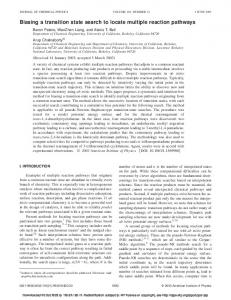
Fig. 4 PES for collinear HwHwNwC conÐguration with CN bond length optimized

The summation of N (E) for i \ 1È40 excluding those shown in Fig. 3 gives the N(E) for even parity shown iin Fig. 5. The N(E) for odd parity shown in the Ðgure are obtained in the same way. The total N(E) is simply the summation of N (E) for even and i odd parities. From the Ðgure, we can see that N(E) is very slightly oscillatory, not as smooth as that for the H ] OH reaction.38 Fig. 6(b) shows the huge di†erence between 2 ] OH in the low-energy region. The N(E) for the H ] CN N(E) for H ] CN and H 2 2 that for the H ] OH reaction for energy lower than 2 0.14 reaction is much smaller than 2 eV. The implies the tunneling e†ect in the H ] OH reaction is much more signiÐcant 2 than that in the H ] CN reaction. 2 The N(E) for the D ] CN reaction for energies up to 0.4 eV is shown in Fig. 6 2 H ] CN reaction. First, we can see the N(E) curve for the together with that for the 2 slight oscillatory behavior, like that for the H ] CN D ] CN reaction also shows 2 reaction. For energy higher than 0.16 eV, the N(E) for the D ] CN reaction is2 higher 2 than that for the H ] CN reaction because of the larger density-of-states for D ] CN 2 2 in the transition state region. For energies lower than about 0.16 eV, where tunneling e†ects are dominant, the N(E) for the D ] CN reaction becomes smaller than that for 2 the H ] CN reaction because of the heavier mass of the D atoms. 2 3.3 Thermal rate constants The thermal rate constant can be calculated from the cumulative reaction probability via a Boltzmann average,

P

`=

dE e~E@kBTN (E) (14) tot ~= where Q (T ) is the reactant partition function (per unit volume), N (E) is the total r reaction probability, tot cumulative k(T ) \ [2pQ (T )]~1 r

N (E) \ ; (2J ] 1)N (E) tot J J

(15)

Quantum transition state wavepacket method

114

Fig. 5 Cumulative reaction probability N(E) as a function of total energy for the H (even 2 reacrotation) ] CN ] HCN ] H reaction, compared with that for the H (even rotation) ] OH 2 tion : (a) linear scale ; (b) logarithmic scale

with J being the total angular momentum. Since the calculation of the N (E) alone J/0 takes more than 1 month of CPU time on an SGI R10000 processor, it is obviously not feasible to calculate the total cumulative reaction probability by using the same method with our current computer power. Thus we invoke the energy shifting approximation to calculate the approximate rate constant from the exact N (E). Since the reaction has a J/0be calculated as56,57 linear transition state, the approximate rate constant should

P

Qt Ct = dEe~E@kB TN (E) (16) (E) B rot J/0 energy shifting 2nQ (T ) ~= r where Qt is the rotational partition function for the linear H CN(D CN) complex at rot 2 the (transition state) saddle point and can be easily calculated as2 k

Qt \ ; (2J ] 1)exp([EJ /k T ) with EJ \ Bt J(J ] 1) (17) rot rot B rot rot J where Bt is the rotational constant of the linear reaction complex at the saddle point ; it rot is 0.757 cm~1 for the H CN complex and 0.495 cm~1 for the D CN complex. C” in eqn. 2 2

J. C. L ight and D. H. Zhang

115

Fig. 6 Comparison of N(E) for the H (even rotation) ] CN reaction and the D (even 2 rotation) ] CN reaction2: (a) linear scale ; (b) logarithmic scale

(16) is a kind of bending partition function of a linear (doubly degenerate) transition state. For a linear four atom system, there are two doubly degenerate bending states and C” can be calculated as56 2 exp([+ut/k T ) 2 exp([+ut/k T ) 1 B 2 B ] . (18) 1 [ exp([+ut/k T ) 1 [ exp([+ut/k T ) 1 B 2 B For the H CN complex, ut and ut are 114.6 cm~1 and 562.3 cm~1, respectively. For 2 the D CN 2complex, ut and1ut are 103.5 cm~1 and 398.62 cm~1, respectively. 2 1 2 The rate constants calculated using eqn. (16) are shown in Fig. 7 for temperatures between 200 and 750 K for the H ] CN reaction and for temperatures between 200 2 Also shown in Fig. 7 are the experimental rate and 600 K for the D ] CN reaction. 2 constants for these two reactions.43,45 For the H ] CN reaction, the agreement 2 high-temperature region. As the between the theory and experiment is only good in the temperature decreases, the experimental value becomes increasingly larger than the theoretical one. At T \ 209 K, the experimental value is larger than the theoretical one by a factor of 2.4. For the D ] CN reaction the theoretical rate constants agree quite 2 well with all the available experimental data. However, because there is no experimental value measured at T \ 209 K, it is very hard to say if the theory can agree with experiCt \ 1 ]

116

Quantum transition state wavepacket method

Fig. 7 Comparison of the present theoretical rate constant with the experimental measurements for the H (D ) ] CN reaction 2 2

ment at that low temperature. We also should bear in mind that we invoked the energy shifting approximation to calculate these rate constants from N(E) (J \ 0). The accuracy of this approximation for these two reactions still must be assessed. Meanwhile if we assume that the energy shifting approximation is quite good for these two reactions, then the comparison between theoretical and experimental results indicates that the tunneling e†ect is not signiÐcant enough on the TSH3 PES. We also compare the present rate constant with other theoretical results on the same PES in Fig. 8. In the high-temperature region, all the calculations agree with each other quite well. Over the whole temperature region, the rate constants for the ground initial state agree very well with our results. In the low-temperature region, the present value is slightly higher than that for the ground initial state (at T \ 200 K, the present value is higher than that for the ground initial state by 16%). In the high-temperature region, the rate constant for the ground initial state is slightly higher than the present value (at T \ 700 K, the rate constant for the ground initial state is higher than the present value

Fig. 8 Comparison of the present theoretical rate constant with other theoretical results for the H ] CN reaction 2

J. C. L ight and D. H. Zhang

117

by 10%). It is worth pointing out that the approximation of the thermal rate constant by that for the ground initial state neglects the reagent rotational e†ect on rate constants, whereas it treats the high J e†ect by the CS approximation. On the other hand, the e†ects from initial reagent rotation are treated accurately in the current study, while the high J e†ect is treated quite crudely by the energy shifting approximation. Realizing the essential di†erence in the approximations made in these two calculations, it is quite interesting to see such good agreement between them. It is found in a recent study of the H ] OH reaction39 that in the high-temperature region the rate constant for the 2 ground initial state is slightly higher than the accurate value, whereas in the lowtemperature region the rate constant for the ground initial state is slightly lower than the accurate result. If this is also true for the H ] CN reaction, this would mean that 2 the rate constant from the energy shifting approximation is quite accurate. Finally, we can see that in the low-temperature region the RB (rotating bond) 4-D results47 are slightly higher than the current results, whereas the rate constants obtained from quasiclassical trajectory calculations, which agree very well with the experimental results, are signiÐcantly larger than the current values. The role of the metastable well in the HHNC conÐguration on the TSH3 PES has not been examined as the well might be an artifact. Hence the current results exclude transition states located in this well. However, if the N (E) from these transition states i were included, the e†ect on the overall rate constants would be small. The sum of N (E) i from these states is less than 0.1 for energies below 0.40 eV, and remains between about [ 0.2 and ] 0.6 for energies between 0.40 eV and 0.5 eV. At energies above 0.4 eV the N(E) from the “ true Ï transition states is larger than 15. Thus the contribution from the metastable states, real or not, is not signiÐcant. It also should be noted that the reaction probability from these HHNC conÐgurations might result in formation of the HNC isomer. The current dividing surface lumps the two isomers as “ product Ï since it does not depend on the polar angle of CN with respect to the intermolecular axis. It will be interesting to investigate this possibility in the future.

4 Conclusions We have evaluated the cumulative reaction probability for the reaction of H (D ) with 2 2 for CN for J \ 0 by the TSWP method. We Ðnd that the method is highly advantageous this system because of the relatively high barrier and low density-of-states in the transition state region. The cumulative reaction probability is a smooth function of energy except for contributions from (possibly spurious) transition states located in the metastable HHNC minimum. The thermal rate constants are approximated from N(E) for J \ 0 by the energy shifting approximation. Surprisingly good agreement is obtained between this calculation and two earlier calculations, the Ðrst based on a 4-D RB approximation,47 and the second an exact quantum initial state selected calculation for the ground state system (with initially non-rotating H and CN). However, all three quantum calculations are not in good agreement with 2experiment or with quasiclassical calculations at low temperatures. This suggests (but certainly doesnÏt prove) that the PES might not permit enough tunneling and/or that the zero point energies at the transition state are too large. The agreement with experiment at higher temperatures for both H ] CN and D ] CN is excellent. 2 2 This research was supported in part by a grant from the Department of Energy, DEF602-87ER 13679, and by Academic research grant RP970632, National University of Singapore. References 1 E. Wigner, J. Chem. Phys., 1937, 5, 720. 2 S. Glasston, K. J. Laidler and H. Eyring, T he T heory of Rate Processes, McGraw-Hill, New York, 1941.

118 3 4 5 6 7 8 9 10 11 12 13 14 15 16 17 18 19 20 21 22 23 24 25 26 27 28 29 30 31 32 33 34 35 36 37 38 39 40 41 42 43 44 45 46 47 48 49 50 51 52 53 54 55 56 57

Quantum transition state wavepacket method J. C. Keck, J. Chem. Phys., 1960, 32, 1035. J. C. Keck, Adv. Chem. Phys., 1967, 13, 85. P. Pechukas and F. J. McLa†erty, J. Chem. Phys., 1973, 58, 1622. P. Pechukas, Modern T heoretical Chemistry, ed. W. H. Miller, Plenum, New York, Part B, vol. 2, 1976. B. C. Garrett and D. G. Truhlar, J. Chem. Phys., 1979, 70, 1593. D. G. Truhlar and B. C. Garrett, Annu. Rev. Phys. Chem., 1984, 35, 159. D. G. Truhlar, B. C. Garrett and S. J. Klippenstein, J. Phys. Chem., 1996, 100, 12771. D. H. Zhang and J. Z. H. Zhang, J. Chem. Phys., 1993, 99, 5615. D. Neuhauser, J. Chem. Phys., 1994, 100, 9272. D. H. Zhang and J. Z. H. Zhang, J. Chem. Phys., 1994, 101, 1146. D. H. Zhang and J. C. Light, J. Chem. Phys., 1996, 104, 4544. D. H. Zhang and J. C. Light, J. Chem. Phys., 1996, 105, 1291. W. Zhu, J. Dai, J. Z. H. Zhang and D. H. Zhang, J. Chem. Phys., 1996, 105, 4881. W. H. Miller, J. Chem. Phys., 1974, 61, 1823. W. H. Miller, S. D. Schwartz and J. W. Tromp, J. Chem. Phys., 1983, 79, 4889. J. W. Tromp and W. H. Miller, Faraday Discuss. Chem. Soc., 1987, 84, 441. K. Yamashita and W. H. Miller, J. Chem. Phys., 1985, 82, 5475. J. W. Tromp and W. H. Miller, J. Phys. Chem., 1986, 90, 3482. T. P. Park and J. C. Light, J. Chem. Phys., 1986, 85, 5870. T. P. Park and J. C. Light, J. Chem. Phys., 1988, 88, 4897. T. P. Park and J. C. Light, J. Chem. Phys., 1989, 91, 974. T. P. Park and J. C. Light, J. Chem. Phys., 1991, 94, 2946. D. Brown and J. C. Light, J. Chem. Phys., 1992, 97, 5465. W. H. Thompson and W. H. Miller, J. Chem. Phys., 1995, 102, 7409. W. H. Thompson and W. H. Miller, J. Chem. Phys., 1994, 101, 8620. (a) P. Day and D. Truhlar, J. Chem. Phys., 1991, 94, 2045 ; (b) P. Day and D. Truhlar, J. Chem. Phys., 1991, 95, 5097 ; (c) D. Neuhauser and M. Baer, J. Chem. Phys., 1989, 90, 4351. U. Manthe and W. H. Miller, J. Chem. Phys., 1993, 99, 3411. U. Manthe, T. Seideman and W. H. Miller, J. Chem. Phys., 1993, 99, 10078. U. Manthe, T. Seideman and W. H. Miller, J. Chem. Phys., 1994, 101, 4759. U. Manthe, J. Chem. Phys., 1995, 102, 9204. W. H. Thompson and W. H. Miller, J. Chem. Phys., 1997, 106, 142. H. Wang, W. H. Thompson and W. H. Miller, J. Chem. Phys., 1997, 107, 7194. U. Manthe and F. Matzkies, Chem. Phys. L ett., 1996, 252, 7. (a) F. Matzkies and U. Manthe, J. Chem. Phys., 1997, 106, 2646 ; (b) U. Mauthe and F. Matzkies, Chem. Phys. L ett., 1998, 282, 442 ; (c) F. Matzkies and U. Manthe, J. Chem. Phys., 1998, 108, 4828. D. H. Zhang and J. C. Light, J. Chem. Phys., 1996, 104, 6184. D. H. Zhang and J. C. Light, J. Chem. Phys., 1997, 106, 551. D. H. Zhang, J. C. Light and S. Y. Lee, J. Chem. Phys., 1998, 109, 79. B. Jackson, Annu. Rev. Phys. Chem., 1995, 46, 251. D. H. Zhang and J. Z. H. Zhang, in Dynamics of molecules and chemical reactions, ed. R. E. Wyatt and J. Z. H. Zhang, Marcel Dekker, New York, 1996. T. Seideman and W. H. Miller, J. Chem. Phys., 1991, 95, 1768. I. R. Sims and I. W. M. Smith, Chem. Phys. L ett., 1988, 149, 564. Q. Sun and J. M. Bowman, J. Chem. Phys., 1990, 92, 5201. Q. Sun, D. L. Yan, N. S. Wang, J. M. Bowman and M. C. Lin, J. Chem. Phys., 1990, 93, 4730. M. A. ter Horst, G. c. Schatz and L. B. Harding, J. Chem. Phys., 1996, 105, 2309. T. Takayanagi and G. C. Schatz, J. Chem. Phys., 1997, 106, 3227. J. H. Wang, K. Liu, G. C. Schatz and M. ter Horst, J. Chem. Phys., 1997, 107, 7869. W. Zhu, J. Z. H. Zhang, Y. C. Zhang, Y. B. Zhang, L. X. Zhang and S. L. Zhang, J. Chem. Phys., 1998, 108, 3509. L.-H. Lai, J.-H. Wang, D. C. Che and K. Liu, J. Chem. Phys., 1996, 105, 3332. J. M. Bowman and G. C. Schatz, Annu. Rev. Phys. Chem., 1995, 46, 169. D. C. Clary, J. Chem. Phys., 1991, 95, 7298. J. M. Bowman, J. Zuniga and A. Wierzbicki, J. Chem. Phys., 1989, 90, 2708. D. H. Zhang, Q. Wu, J. Z. H. Zhang, M. Dirke and Z. Bac—ic, J. Chem. Phys., 1995, 102, 2315. D. H. Zhang and J. Z. H. Zhang, J. Chem. Phys., 1994, 100, 2697. Q. Sun, J. M. Bowman, G. C. Schatz, J. R. Sharp and J. N. L. Connor, J. Chem. Phys., 1990, 92, 1677. J. M. Bowman, J. Phys. Chem., 1991, 95, 4960. Paper 8/01188E ; Received 10th February, 1998