The scale representation - Signal Processing, IEEE ... - Columbia EE

IEEE TRANSACTIONS ON SIGNAL PROCESSING, VOL. 41, NO. 12. DECEMBER 1993

3215

The Scale Representation Leon Cohen

Abstract-We consider “scale” a physical attribute of a signal and develop its properties. We present an operator which represents scale and study its characteristics and representation. This allows one to define the scale transform and the energy scale density spectrum which is an indication of the intensity of scale values in a signal. We obtain explicit expressions for the mean scale, scale bandwidth, instantaneous scale, and scale group delay. Furthermore, we derive expressionsfor mean time, mean frequency, duration, frequency bandwidth in terms of the scale variable. The short-time transform is defined and used to obtain the conditional value of scale for a given time. We show that as the windows narrows one obtains instantaneous scale. Convolution and correlation theorems for scale are derived. A formulation is devised for studying linear scale-invariant systems. We derive joint representations of time-scale and frequency-scale. General classes for each are presented using the same methodology as for the time-frequency case. As special cases the joint distributions of Marinovich-Altes and Bertrand-Bertrand are recovered. Also, joint representations of the three quantities, time-frequency-scale are devised. A general expression for the local scale autocorrelation function is given. Uncertainty principles for scale and time and scale and frequency are derived.

I. INTRODUCTION CALE is a physical attribute of a signal just like frequency. For a given signal we may properly ask what is its frequency content. Similarly, we may properly ask what is its scale content. In the frequency case, we determine the frequency content via the Fourier transform; for scale we need a transform which indicates the moment of scale in the signal. It is the purpose of this paper to develop the concept of scale, its representation and properties. The important first step is to have the scale operator and obtain the scale transform. The solution of the eigenvalue problem for this operator gives the scale transform. Subsequently we study this transform and its properties. In analogy with instantaneous frequency and group delay, we will introduce similar concepts for scale. We obtain explicit expressions for mean scale and scale bandwidth and also for instantaneous scale and scale group delay. Convolution and correlation theorems will be derived. We develop methods for obtaining joint representations involving scale [ 11-[6] which are generalizations of the method devised by the

S

Manuscript received September 1, 1992: revised May 26, 1993. The Guest Editor coordinating the review of this paper and approving it for publication was Dr. Patrick Flandrin. This work was supported in part by the United States Air Force at Rome Laboratories under Grant F30602-91c-0120. The author is with the Department of Physics, Hunter College, New York, NY 10021. IEEE Log Number 9212193.

author for the time-frequency case [8]-[ 101. Also, we derive a joint representation involving time-frequency-scale. A fundamental attribute of frequency and time is their relation with the translation of functions and this leads to the study of linear shift invariant systems. The fundamental property of scale is that of compression; hence, we develop the methodology for linear scale invariant systems. We show that the scale operator does not commute with the time operator or frequency operator. This implies that there must be an uncertainty principle between timescale and frequency-scale. We will derive these uncertainty principles and obtain the minimum uncertainty signal. The use of operator methods in signal analysis has recently been devised for arbitrary physical variables [ 11, [2], [7]. The basic method is based on the work of Scully and Cohen [l 13. We apply this method to be the study of scale. Scaling has been an imoprtant concept in a number of fields. In the general theory of wavelets the concept of scale enters in a fundamental way. This has led to many issues regarding the concept “scale” and in particular has led to ideas regarding joint representations of time and scale. Scaled functions also appear in radar and sonar and in particular in the study of the wide band ambiguity function and also in the study of optical imaging. See [12][ 191 and references therein. 11. REPRESENTATION OF SIGNALS AND OPERATOR METHODS The basic reason for expressing a signal in another domain or representation is that very often that will reveal properties of the signal which may not be apparent in the time domain. Another important reason is that the production, propagation, or behavior of a signal may depend upon physical quantities other than time. Therefore to see how a signal behaves under those circumstances one expresses the signal in the representation in question, does the analysis, and then transforms back to the time domain. In addition, if we want to construct signals with characteristics relating to a certain physical property, we obviously construct the signal in the representation of that quantity and then transform back to the time domain. Representations are usually associated with a physical quantity. In the case of the Fourier representation, the physical quantity is frequency. In the same manner we will develop the scale representation which will represent a signal in a domain for which the fundamental physical

1053-587X/93$03,00 0 1993 IEEE

IEEE TRANSACTIONS ON SIGNAL PROCESSING, VOL

3216

variable is scale. We have recently developed a general approach for associating physical quantities with operators [ 11, [6], [7] similar to the methods used in other fields [20], [21]. This leads to a methodology for constructing and studying representations, particularly joint representations. We review here some basic operator methods.

A. Operators Suppose we have an operator Q. which represents or is associated with a physical quantity. Operators which represent a physical quantity will generally be Hermitian. That means that for any two functionsf(t) and g ( t ) ,

'

s

g*(t)Q.f dt =

s

f ( t ) ( Q . g ( t ) ) *dt.

Q.u(a, t )

au(a, t)

=

(2.2)

results in the eigenfunctions, u ( a , t ) and eigenvalues, a . Since the operator is Hermitian the eigenvalues are real and the eigenfunctions are complete. This implies that

5

u ( a , t ) u * ( a , t ' ) da

s

=

6(t - f');

u ( a , t ) u * ( a ' , t ) dt = 6 ( a - a ' ) .

(2.3)

[ 3 , W] = 3W

f ( f ) u * ( a , t ) dt.

(g) =

3

=j

d W dw '

-.

d dt

= w

s

g ( 4 1"2

da.

(2.9)

To evaluate, one first obtains the transform F ( a ) and then evaluates the integral. However, one does not have to find F(a)!-it can be done directly from the time function by way of

(g)

= S f * ( t ) g ( ~ . ) f (dt. ~

(2.10)

The equality of the right hand sides of (2.9) and (2.10) is well known; we give a simple proof here for those readers not familiar with this result. Substituting,f(t) as given by (2.4) into (2.10) we have (g) =

ss

F * ( a ' ) u * ( a ' , t ) g ( Q ) F ( a ) u ( a ,t ) dt da' da.

=

s5 s ss

=

g ( a ) u ( a , t ) and hence,

F * ( a ' ) u * ( a ' , t ) g ( a ) F ( a ) u ( a ,t ) dt du' da (2.12)

F * ( a ' ) g ( a ) F ( a )6 ( a - a ' ) da' da

(2.5)

We shall use the double arrow to signify correspondence of the time function and its transform, f ( t ) e F ( a ) . The time and frequency operators 3 and W are [lo]

3 = t W = -j

(2.8)

B. Averages Perhaps the most important reason for the power of the operator method is that one can calculate averages in a very easy way. If we have a function of a , g ( a ) , then its average is2

Now, g ( Q . ) u ( a , t )

where u ( a , t ) is the transformation matrix or basis kernel and F ( a ) is the representation of the time function in the a domain. The inverse transformation is

s

W3 = j .

Operators representing other physical variables will usually be expressed in terms of the time and frequency operators. As we will see that is the case for the scale operator.

(8)=

=

-

(2.11)

Therefore, any time function can be expressed as

F(a)

NO 12, DECEMBER 1993

They satisfy the fundamental commutation relation [ 101

(2.1)

Now, if the operator is Hermitian then the solution of the eigenvalue problem

41.

(time domain),

(2.6)

(frequency domain).

(2.7)

C. Characteristic Function Operator For a density P ( a ) , the characteristic function of a is defined by

M ( a ) = (e""") =

s

e J " " P ( a )da.

(2.14)

The characteristic function uniquely determines the distribution, (2.15)

'Operators will be denoted by calligraphic letters. The commutator of two operators, 0 and 63, will be denoted by the standard notation, [a, 631 = a63 - 030. Indefinite integrals imply an appropriate region of integration which depends on the representation being considered. Since the scale operator will give a continuous spectrum we explain the basic method assuming a continuous spectrum. In (2.2) we have assumed that the operator is expressed in the time representation, although the eigenvalue problem can be solved in any representation. In that case the operator must be expressed in the representation of interest. Also, we assume basis sets are self reciprocal.

Since the characteristic function is an average, the average of eJa"",it can be calculated using (2.10), M(a) =

f*(t)e'"'f(t) dt,

(2.16)

'The reason for taking I F ( a ) l Lto be the density is discussed in detail in references _111, _ 121. . _171. . _

COHEN: THE SCALE REPRESENTATION

3211

where Q. is the operator corresponding to the variable a . Now, We call eJaa the characteristic function operator. To show ejoe t n explicitly that o leads to the density given by IF(a)I2 expressf(r) in terms of its transform to obtain

m

- c -( jk!a I k

F ( a ) u ( u ,t) da' du dr. But e j a a u ( a ,r) M(a) =

=

s

(2.17)

e j a a u ( u ,r ) , giving

F * ( u ' ) e J a U6(u

-

ejUef(t) = eJue C a n t n

a ' ) F ( a )da' da

111. THE SCALEOPERATOR The fundamental quantity that characterizes a representation is the operator. We take the following operator for scale =

l(3W

+ W3)

(3.1)

and we use the lower case c to represent scale values. The following basic relations show that it scales or compresses functions of time, f ( t ) , and frequency F ( w ) ,

C a,eo(n+l/*)tn

-

(2.18)

which shows that

e

(3.7) To obtain the action of eJoe on an arbitrary functionf(t), we expand the function in a power series

IF(u)(2e'a"da,

=

ektn

k=O

=

e"/*f(e

r). (3.8)

The scale operator is adopted from the theory of quantum optics where it is written in terms of the creation and annihilation operators [22]. It is related to the affine group [17]-[19]. Also, Klauder [23] has used it to study path integrals and quantum g r a ~ i t y . ~ By using (2.8) the scale operator can be written in the following alternate ways

e

=

3w

- I2 J' g =

w3 + 1'9, 2J

(3.9)

where 9 is the unit operator. A. Basic Properties of Scale and time do not commute, In fact

[3, e ] = j 3 . ejuef(t)

ejoe ~ ( w = ) e-"/*F(e-"w).

(3 '2)

Also, ej In

uef

(3.10)

= e'/2f(eut);

(r)

=

&f (ut);

The significance of this is that we can not find a common representation which diagonalizes both the scale and time operators. In addition, it shows that we must have an uncertainty principle as discussed in Section XIV. However, time commutes with the commutator of time and scale (3.11)

The operator, eJ" therefore compresses the independent variable. It may be called the compression operator. The significance of the factor, e o / 2 ,is that it preserves normalization and the reason it entered in an automatic way is because the operator, elue is unitary. The compression operator should be contrasted with the translation OPerators for time and frequency functions, e''wf(t)

= f f da.

(15.13)

(15.14)

This distribution was derived by Marinovich [16], [171 and Altes [ 141 by different methods. These distributions satisfy the marginals of time and scale,

S

P ( t , c) dc = I s(t)I2.

(15.15)

XVI. JOINT FREQUENCY-SCALE REPRESENTATIONS We now find representations of frequency and scale. However we emphasize that we are seeking representations of frequency and time scaling. In section XIX, we will address the issue of frequency scaling. The notation we shall use is M ( 7 , a) and P ( u , c) for f * ( e - ~ / 2 t ) e j s r ~ f e adt. / 2 t ) (15.10) the frequency-scale characteristic function and distribuexp (jeeo/2t)e"/2f(e"t)dtf

som

(15.9)

COHEN: THE SCALE REPRESENTATION

3287

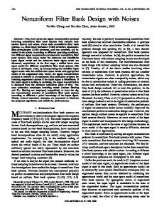
TABLE I1 FREQUENCY-(f) SCALE REPRESENTATIONS #

Characteristic Function: M ( T , a )

Ordering

Distribution: P ( w , c )

A cosh ( o / 2 )) du

F(&'

Table 1 and 2 give, respectively, joint time and frequency representation with time scaling [(t)scale]

tion respectively. They are related by

M(T,a)

=

ss

e"w+jOcP(w,e) dw de. dt da.

(16.1) (16.2)

The characteristic function will be obtained from the chara; , W, e )by averaging acteristic function operator, m ( ~ it

M(7,a> =

(m(7, 0, w, e )

so

(16.3)

m

=

f * ( t ) W ~ , a; W , e)f(t)dt.

(16.4)

We could repeat the algebra as in the previous section; however there is a simple procedure to evaluate these cases. First we note that we can evaluate M(T,a) in the Fourier domain,

1

m

M(7,a)

=

F*(w)m(~, a; W, e ) F ( w ) dw

(16.5)

-m

We are assured that evaluating M by way of (16.4) or (16.5) will give the identical results since which representation is used is immaterial in calculating averages by the operator method. Now, note that structurally m(7, a; W , e ) F ( w ) is identical to m(O, a; 3, e ) f ( t ) except for the fact that a goes into -a. Therefore the frequencyscale characteristic function will be identical in form to the time-scale characteristic function, but we must change the sign of a and replace the time function by its Fourier transform. Also, we must change O to T. The distribution is the Fourier transform of the characteristic function. Since everything is structurally the same except for the minus sign in a, we can obtain the frequency-scale distri-

bution from the time scale distribution by replacing c by -e, and t by w and replace the signal with its Fourier transform. We should emphasize that the limits of integration on the frequency variable go from - 03 to 03 since the spectrum is not constrained. (In Section XIX we will deal with frequency scaling where the spectrum will have only positive values .) Table I1 lists the corresponding characteristic function operators, characteristic functions and the distributions corresponding to the ordering cases we have considered in Section XV. The frequency-scale distributions satisfy the marginal of frequency and scale,

s1

P ( w , e) dw

=

(D(c)I2;

(16.6)

P ( w , e ) de

=

IF(w)I2.

(16.7)

XVII. GENERAL CLASSOF JOINT SCALE REPRESENTATIONS The method we present for obtaining the general class of time-scale distributions is a generalization of the method used to obtain the general class of time-frequency distributions [8]-[ 101. We start with any particular characteristic function and define a new characteristic function by Mn,,(O,

a> =

+(e,

a)M(O, 4

(17.1)

where 4 is the kernel function whose role is identical to the time-frequency case. The general class is then

(17.2) We emphasize that M is any particular characteristic function.

IEEE TRANSACTIONS ON SIGNAL PROCESSING, VOL. 41, NO. 12, DECEMBER 1993

3288

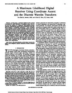
TABLE 111 FREQUENCY-(U) SCALEREPRESENTATIONS #

Ordering

Characteristic Function: M ( 7 ,

Distribution: P ( w , e )

U)

. F(eo/*

2 sinh ( u / 2 ) p (.-a/' cosh (u/2)

. F(ea/'

w cosh ( u / 2 )

Suppose we chose the characteristic function given by ordering one, then 1 P ( t , c) = 4n2 -

[ [[f *

+(e, a)) f

(e"/2U)

exp (-jet - jac jeu +

(e-"/2u)dB du da.

(17.3)

class and any other distribution is obtained by appropriate choice of the kernel. So for example, if we chose the kerne1 equal to one then we obtain the Bertrand-Bertrand distribution while if we chose the kernel to be the inverse of that given by (17.5) then we obtain the Marinovich-Altes distribution. The identical considerations leading to the time-scale general class will give the general frequency-scale class.

The particular distribution is obtained, as in the time frequency case, by specifying the kernel. If, for example we take the kernel to be equal to one then we obtain the distribution of Marinovich and Altes. If we take a kernel given by

.

-joc

dr da.

(17.6)

som

f * (e-"/2t)ejetf (e"I2t) dt

+(e, 4 =

[

exp [2j& sinh ( a / 2 ) / 0 ] f * ( e - " / ~ t ) f ( e " / ~ tdr )

then one obtains the Bertrand-Bertrand distribution. Note that this kernel is a functional of the signal. That should not be surprising because that is also the case with the time frequency case [6]-[lo], although for most of the time frequency cases that have been considered, the kernel is not a functional of the signal. If we chose the characteristic function given by ordering 2 then

P ( t , c> =

4 'j 'j 'j f * ( e - " / 2 u ) + ( e , 4n exp [-jet - jac

Choosing M as given by ordering one we have

P(u, c ) =

(17'5)

Equation (17.3) or (17.5) may be considered a general

4n2

SSS

F*(eg/2u) exp (-jTt

+ ( r , a)F(e-"l2u)dfl du do.

+ jac + jru) (17.7)

If we choose M as given by ordering two we obtain P(u, c)

a)

+ 2jBu sinh ( a / 2 ) / a ]

f (e"/2u)d8 du da.

(17.4)

m

=

1 [[ 4n

S

F*(e-"/2u)d(r, a)

exp [-jrt

+ joc + 2 j ~ usinh ( a / 2 ) / o l

F(e"/2u)dr du da.

(17.8)

For the time frequency case the conditions on the kerne1 have been studied and developed in detail [441-[491.

COHEN: THE SCALE REPRESENTATION

3289

TABLE IV

TIME-(U) SCALE REPRESENTATIONS #

Characteristic Function: M ( 0 , U )

Ordering

Distribution: P ( r , c)

Tables 3 and 4 give the distributions of frequency and time for frequency scaling [(w)scale]. D ( c ) and D , are the time and frequency scale transforms.

Generally speaking, the same ideas apply to other representations. For example, the conditions to satisfy the marginals and instantaneous scale are identical to the conditions for satisfying the marginals and instantaneous frequency in the time-frequency case.

A. Transformation of Distributions For the time-frequency case the general relation between distributions was first derived in reference [9]. We now do the same for the distributions we have derived for scale. Suppose we have two time-scale distributions PI and P2 with corresponding kernels 41and 42.Their characteristic functions are ~ ~ (a)0=,

+we,

~ ~ (a)0=, 42(e,a ) w e ,

0); 0).

function [ l ] , [lo], [44]. We now show that the same can be done for scale. We prove that the general time-scale distributions can be written in the form

P ( t , c) with &(a) =

2n

SS

$(e,

Rr(a)e-"" da

(17.13)

a)M(B, a)e-'@' de.

1 2a

1S

eJe('-')+(f?,a ) f * ( e - " / 2 u ) f ( e " / 2 udu ) dB (17.15)

Hence,

By taking the Fourier transform of both sides one obtains

P l ( t , c) =

Ss

g ( t ' - t , c' - c)P2(t',c ' ) dt' dc' (17.11)

with

. 4(0, a) f * ( e - " / 2 u )f (e"/2u)du de.

(17.16)

XVIII. JOINTREPRESENTATIONS OF TIME-FREQUENCYSCALE We now consider joint representations of the three variables time, frequency, and scale. There are many orderings possible; we consider only one here and using it we write the general class. Take

X(8, B. Local Autocorrelation Method A very fruitful approach to study time-frequency distributions has been to generalize the relationship between the energy density spectrum and the deterministic autocorrelation function by defining a local autocorrelation

(17.14)

We shall call R, the generalized local scale autocomelation function. Depending on which definition we use for the general class (17.3)-( 17.5) we have respectively &(a) = -

(17.9)

1 2n

-

'S

= -

7,

a) = e

j o W / 2 jO3+jrW

e

ejuW/2 .

(18.1)

The characteristic function evaluates to [ 11 M(e,

7,

=

:S *

1

,jerf*(e-u/2(t - n)

f (e"/'(t

+ ;7)) dt.

(18.2)

IEEE TRANSACTIONS ON SIGNAL PROCESSING. VOL. 41, NO. 12, DECEMBER 1993

3290

The distribution is

. exp (-jet

- jrw

-

jab) db' da dr (18.3)

which gives

A N D SCALING I N OTHER XIX. FREQUENCY-SCALING DOMAINS We have considered the scaling of time and have defined the operator e to be the time scaling operator. Equally well one can consider the scaling of frequency functions. It is clear from (3.3) that the operator for frequency scaling is, e, = -e and its eigenfunctions are yw(c, w ) which are the same form as the time scaling eigenfunctions with t replaced by w . For the frequency scaling representation only the positive half of the spectrum is considered, which is equivalent to considering analytic signals. The transformation properties from the frequency domain to the scale domain are now

To obtain the general class of time-frequency-scale distributions we multiply the characteristic function by a kernel of three variables, +(e, r , a) to obtain the generalized characteristic function

r , a)

Mnew(e9

=

4(b'> r7

', a).

(18.5)

If we use (18.2) for M we have

ejorf*(e-g/2(t - 1 2 7))

Mnew(O,r , a) = 4(e, r , a)

f(e"/'(t

+ i r ) ) dt.

(18.6)

and the general class is therefore

-

exp (-jet

-

jrw - jac) db' da dr. (18.7)

Explicitly,

e -j c In w dw .

Now, everything we have done for the time cases can be directly transliterated to this situation with of course a different interpretation. In particular we can define the shortfrequency scale transform by e -jc In r F ( T ) H ( T- U ) -dr (19.3)

J;

where H ( w ) is the window function in the frequency domain. The joint distribution of frequency and frequencyscale is then P ( t , c) = 1 D, (c)1'. The same method leading to instantaneous scale now leads to the conditional scale for a given frequency given by w $ ( w ) . This differs from scale for a given frequency for the time scaling case by a minus sign. The other quantities such as average scale etc. are obtained the same way except that the limits of integration run from 0 to 00 in frequency. Also one can define the density of frequency for a given time by using the short time Fourier transform, e - J C ~In w E,(c) = e-J"y(r)h(r - t ) dr dw 2a 0 J;J

i

- jrw -

jac] db' da dr du.

(18.8)

(19.2)

Sm j

~

The joint distribution of time and frequency-scaling is then given by P ( t , c,) = 1 Ef(cw)1'.

A . Joint Frequency Frequency-Scale Representations In Sections XV-XVII, we obtained joint representations of time and time-scale and frequency and time-scale. We now address how to obtain joint representations of (18.9) P ( t , w , c) dc = P ( t , U), frequency and frequency-scale and time and frequencyscale. Let us first consider the case of frequency and fre(18.10) quency-scaling. The characteristic function will involve P ( t , w , c) dt = P ( w , c ) , the frequency and scale operator. From a mathematical point of view there is no difference to the previous work (18.11) as long we transliterate appropriately. In fact, all we have P ( t , U , c) dw = P ( t , c ) , to do is to change time to frequency, the signal, f ( t ) to where the marginals as given by the right hand side of frequency functions, F ( w ) . We have already considered (18.9)-( 18.1l ) , are the general classes of time-frequency, the evaluation of such characteristic functions in Section frequency-scale and time-scale distributions. XVI where we considered distributions to frequency and This general class of time-frequency-scale distributions satisfies

s som S

COHEN: THE SCALE REPRESENTATION

3291

time scaling. However there the function F(w) was the Fourier transform of the signal and in that case it ranged over the whole frequency axis. Now the function, F ( o ) is arbitrary but can only range from zero to infinity. Therefore all we have to do is take the results of Table I1 and make the limits of integrations zero to infinity. Similarity to obtain distribution of time and frequency scaling we take the results of Table I and let the limits of integration go from - 03 to 03. These are cataloged in Tables I11 and IV . All other consdieration regarding joint representation with frequency scaling can be done the same way. We write here the general classes analogous to (17.3),

exp ( -jrw - jac,,

+ jru) 4

F(e-“I2u)dr du da

*

(7,

U)

(19.4)

and also the one analogous to and ( 17.5).

exp [-jrw

-

jac,,. + 2j7u sinh (a/2)/a]

. F(e“/’u)dr du da

(19.5)

In the above two equations we have used c, to emphasize that we are doing frequency scaling.

B. Other Domains In the above, we have shown how to handle frequency scaling. We now want to discuss how to do scaling for an arbitrary domain or physical variable. Suppose the physical variable is a and the functions in that domain are F ( a ) . We define the generalized scaling operator by (19.6)

and in general we have that

REFERENCES L. Cohen, “A general approach for obtaining joint representations in signal analysis and an application to scale,’’ Advanced Signal-Processing Algorithms, Architectures and Implementaiion I I , Franklin T . Luk, Ed., Proc. SPIE, vol. 1566, pp. 109-133, 1991. -, “Convolution, filtering, linear systems, the Wiener-Khinchin theorem: Generalizations,’ ’ Advanced Signal-Processing Algorithms, Architectures and Implementation I t , Franklin T . Luk, Ed., Proc. SPIE, vol. 1770, pp. 378-393, 1992. -, “Scale, frequency, time, and the scale transform,” in Proc. 6ih IEEE Signal Processing Workshop Statisiical Signal and Array Processing, Victoria, B.C., Canada, 1992, pp. 26-29. -, “Instantaneous scale and the short-time scale transform,” in IEEE Signal Processing In?. Symp. Time-Frequency and Time-Scale Anal., 1992, pp. 383-386. -, “Scale and inverse frequency representations,” in The Role of Wavelets in Signal Processing, B. W . Sutter, M. E. Oxley, and G . T . Warhola, Eds. Wright-Patterson Air Force Base, OH: AFIT, 1992, pp. 118-128. -, “Instantaneous anything,” in Proc. IEEE Int. Con$ Acousi., Speech, Signal Processing-ICASSP ’93, pp. IV105-VlO8. -, “A general approach for obtaining joint representations in signal analysis,” submitted to Proc. IEEE, 1992. -, “Generalized phase-space distribution functions,” J . Math. Phys., vol. 7 , pp. 781-786, 1966. -, “Quantization problem and variational principle in the phase space formulation of quantum mechanics,” J . Math. Phys., vol. 17, pp. 1863-1866, 1976. -, “Time-frequency distributions-A review,” Proc. IEEE. vol. 77, pp. 941-981, 1989. M. Scully and L. Cohen, “Quasi-probability distributions for arbitrary operators,” in The Physics of Phase Space, Y. S . Kim and W . W. Zachary, Ed. New York: Springer-Verlag, 1987. E. J. Kelly and R. P. Wishner, “Matched filter theory for high velocity, accelerating targets,” IEEE Trans. Mil. Electronics, vol. MIL9 , pp. 56-69, 1965. R. A. Altes, “The Fourier-Mellin transform and Mammalian hearing,” J . Acoustic. Soc. A m . , vol. 63, pp. 174-183, 1978. -, “Wide-band, proportional-bandwidth Wigner-Ville analysis,” IEEE Trans. Acoust., Speech, Signal Processing, vol. 38, pp. 10051012, June 1990. G. Eichmann, and N. M. Marinovich, “Scale-invariant Wigner distribution and ambiguity functions,” in Proc. In?. Soc. Opt. Eng. SPIE, vol. 519, pp. 18-24, 1984. N. M. Marinovich, “The Wigner distribution and the ambiguity function: Generalizations, enhancement, compression and some applications,” Ph.D. dissertation, City Univ. New York, New York, NY, 1986. [ 171 J , Bertrand and P. Bertrand, “Representation temps-frequence des signoux,” C. R. Acad. S c i . , vol. 299, serie 1, pp. 635-638, 1984. [I81 -,, “Time-frequency representations of broad band signals,” in The Physics of Phase Space, Y. S . Kim and W. W. Zachary, Ed. New York: Springer-Verlag, 1987, pp. 250-252. [I91 “Affine time-frequency distributions,” in Time Frequency Signal Analysis-Meihods and Applications, B. Boashash, Ed. London: Longman-Chesire, 1992. [20] H. Margenau and G . M. Murphy, The Mathemaiics of Physics and Chemistry. Princeton, NJ: Van Nostrand, 1959. [21] E. Merzbacher, Quantum Mechanics. New York: Wiley, 1970. [22] P. Meystre and M. Sargent 111, Elements of Quantum Opiics. New York: Springer-Verlag, 1990. [23] J. R. Klauder, “Path integrals for affine variables,” in Functional Integraiion: Theory and Applications, J . P. Antoine and E. Tirapgui, Eds. New York: Plenum, 1980. [24] Morse and Feshbach, Methods of Theoretical Physics. New York: McGraw-Hill, 1953. [ 2 5 ] L. Cohen, “Transformation of operators,” Amer. J . P h y s . , vol. 34, pp. 684-690, 1966.

-.

eJUeaF(a) = e“/2F(e“a); e””“eaF(a)= & f ( u a ) .

XX. CONCLUSION We have presented the basic properties of scale and treated it as a physical variable like frequency and we have given a framework for obtaining joint representations involving scale.

(19.7)

It is clear that nothing we have previously done for time scaling is particular to the time variable. Everything can be carried over directly. To convert the equation we have derived for time scaling to scaling in the “a” domain arbitrary variables a , all we have to do is substitute a for t and f ( a ) for f ( t ) in any of formulas we have obtained. The above discussion for the frequency case is an example.

IEEE TRANSACTIONS ON SIGNAL PROCESSING, VOL. 41, NO. 12, DECEMBER 1993

-, “Operator transform pairs,” to be submitted to IEEE Trans. Informat. Theory. U. K. Laine, “Famlet, To be or not to be a wavelet,” in IEEE Signal Processing Symp. Time-Frequency and Time-Scale Analysis, 1992, pp. 335-338. R. G . Baraniuk and D. L. Jones, “Unitary equivalence: A new twist on signal processing,” submitted to IEEE Trans. Signal Processing, 1993. -, “Warped wavelet basis: Unitary equivalence and signal processing,” in Proc. IEEE Int. Conf. Acoust.. Speech and Signal Processing-ICASSP ’93, pp. 111320-111323. L. Cohen, “The covariance of a signal,” in preparation. L. Cohen and C. Lee, “Instantaneous bandwidth,” in Time Frequency Signal Analysis-Methods and Applications, B. Boashash, Ed. London: Longman-Chesire, 1992. D.Gabor, “Theory of communication,” Jour. IEE, vol. 93, pp. 4294 5 7 , 1946. J. Ville, “Theorie et applications de la notion de signal analytique,” Cables et Transmission, vol. 2A, pp. 61-74, 1948. 0. Rioul, “Wigner-Ville representations of signal adapted to shifts and dilations,” AT&T Bell Lab. Murray Hill, NJ, Tech. Memo., 1988. T. E. Posch, “Wavelet transform and time-frequency distributions,” Advanced Algorithms and Architectures f o r Signal Processing IV, Franklin T . Luk, Ed. Proc. SPIE, vol. 1152, pp. 477-482, 1989. 0. Rioul and P. Flandrin, “Time-scale energy distributions: A general class extending wavelet transforms,” IEEE Trans. Signal Processing, vol. 4 0 , pp. 1746-1757, July 1992. A. Papandreaou, F. Hlawatsch, and G . F . Boudreaux-Bartels, “Quadratic time-frequency distributions: The new hyperbolic class and its intersection with the affine class,” in Proc. 6th IEEE Signal Processing Workshop Statistical Signal and Array Processing, Victoria, B.C., pp. 26-29, 1992. R. G . Shenoy and T . W. Parks, “Wideband ambiguity functions and the affine Wigner distributions,” submitted to EURASIP Signal Processing, 1993. R. G . Baraniuk and L. Cohen, “Operator methods and unitary equivalence,” to be submitted. J . Jeong and W. J. Williams, “Variable windowed spectrograms: Connecting Cohen’s class and the wavelet transform,” in ASSP Workshop Spectrum Estimation and Modeling, pp. 270-273, 1990. P. Flandrin, “Scale invariant Wigner spectra and self-similarity,” L. Torres, E. Masgrau, and M. A. Lagunas (Ed.), Signal Processing V . New York: Elsevier. 1990.

-, “On the time-scale analysis of self similar processes,” in The Role of Wavelets in Signal Processing, B. W. Sutter, M. E. Oxley, and G . T. Warhola, Eds. Wright-Patterson Air Force Base, OH: AFIT, 1992, pp. 137-150. R. M. Wilcox, “Exponential operators and parameter differentiation in quantum physics,” J . Math. P h y s . , vol. 8 , pp. 962-982, 1967. H. I. Choi and W . J. Williams, “Improved time-frequency representation of multicomponent signals using exponential kernels,” IEEE Trans. Acoust. Speech Signal Processing, vol. 37, pp. 862-871, June 1989. J. Jeong and W. J. Williams, “Kernel design for reduced interference distributions,” IEEE Trans. Signal Processing, vol. 4 0 , pp. 402-412, Feb. 1992. P. J. Loughlin, J. Pitton, and L. Atlas, “Bilinear time-frequency representations: New insights and properties,” IEEE Trans. Signal Processing, vol. 4 1 , pp. 450-467, Feb. 1993. S . Oh, R. J . Marks, 11, L. E. Atlas, and J. A. Pitton, “Kernel synthesis for generalized time-frequency distributions using the method of projection onto convex sets, ’’ Advanced Algorithms and Architectures f o r Signal Processing I l l , Franklin T. Luk, Ed., Proc. SPIE, vol. 1348, pp. 197-207, 1990. Y . Zhao, L. E. Atlas and R. J. Marks 11, “The use of cone-shaped kernels for generalized time-frequency representations of nonstationary signals,” ZEEE Trans. Acoust. Speech Signal Processing, vol. 38, pp. 1084-1091, 1990. R. G . Baraniuk and D. L. Jones, “Optimal kernels for time-frequency analysis,” Advanced Algorithms and Archirectures f o r Signal Processing 111, Franklin T . Luk, Ed., Proc. SPIE, vol. 1348, pp. 181-187, 1990.

Leon Cohen was born in Barcelona, Spain on March 2 3 , 1940. He received the B.S. degree from City College of New York, New York, NY in 1958 and the Ph.D. degree from Yale University, New Haven, CT in 1966. He has contributed to the fields of astronomy, quantum mechanics, mathematics, chemical physics and signal analysis. Dr. Cohen is a fellow of the American Physical Society.