The Search for Active Marsquakes Using Subpixel Coregistration and

Journal of Geophysical Research: Planets RESEARCH ARTICLE 10.1029/2018JE005649 Key Points: • Best practice of identifying coseismic displacement in HiRISE images of Mars produces images coregistered with about 1/50 pixel accuracy • No strong evidence of detectable coseismic displacement in part of Cerberus Fossae over 8 years of observations • Ancillary observations of recurring slope lineae activity do not match previous seasonal timescales

Supporting Information: • Supporting Information S1 • Movie S1 • Movie S2 • Movie S3 • Movie S4 • Movie S5 • Movie S6 • Movie S7 Correspondence to: P. M. Grindrod, [email protected]

Citation: Grindrod, P. M., Hollingsworth, J., Ayoub, F., & Hunt, S. A. (2018). The search for active marsquakes using subpixel coregistration and correlation: Best practice and first results. Journal of Geophysical Research: Planets, 123, 1881–1900. https://doi.org/10.1029/ 2018JE005649 Received 19 APR 2018 Accepted 1 JUN 2018 Accepted article online 10 JUN 2018 Published online 26 JUL 2018

The Search for Active Marsquakes Using Subpixel Coregistration and Correlation: Best Practice and First Results Peter M. Grindrod1

, James Hollingsworth2,3

, Francois Ayoub4

, and Simon A. Hunt5

1

Department of Earth Sciences, Natural History Museum, London, UK, 2ISTerre, Université Grenoble Alpes, Grenoble, France, ISTerre, CNRS, Grenoble, France, 4Seismological Laboratory, California Institute of Technology, Pasadena, CA, USA, 5 Department of Earth Sciences, University College London, London, UK 3

Abstract The state of seismic activity on Mars is currently unknown. On Earth, coseismic displacement has been observed using visible wavelength images and subpixel coregistration and correlation techniques. We apply this method to Mars with the COSI-Corr (Co-registration of Optically Sensed Images and Correlation) software package using High-Resolution Imaging Science Experiment (HiRISE) images, focusing on part of the Cerberus Fossae fault system. We derive best practices for applying this method to the study of coseismic displacements on Mars. Using a time series of eight overlapping HiRISE images, we achieve pixel coregistration with a mean accuracy of about 1/50 of a pixel. We see no clear evidence for coseismic displacement in this region during a time period of over 8 years. One possible displacement signal (1–2 m of west-east displacement over a length scale of about 50 m) that has similarities to terrestrial coseismic deformation was dismissed as the result of incomplete correction of steep topography during the coregistration stage. Ancillary observations of recurring slope lineae (RSL) activity in the surrounding fault system offer no supporting evidence for the occurrence of coseismic displacement but do seem to suggest RSL activity that does not fit into previous seasonal timescales. Although it is unlikely that we have observed coseismic displacement in our study area during this time period, the best practice method and the accuracy of our results offer encouragement for future studies. HiRISE, Context Camera, and Color and Stereo Surface Imaging System images can be used to complement and independently verify in situ seismic observations by the InSight (Interior Exploration using Seismic Investigations, Geodesy, and Heat Transport) lander or source location changes from the ExoMars Trace Gas Orbiter spacecraft.

Plain Language Summary It is currently unknown whether there are active “marsquakes”— earthquakes on Mars—despite past missions with seismometer instruments designed for their detection. In this study we compare images of Mars taken over 8.5 (Earth) years to look for changes at the surface that could have been caused by marsquakes. We focused our study on the youngest fault system on Mars, Cerberus Fossae, as it is one of the areas that probably has the best chances of being active today. We developed a method that should be sensitive to small changes in the surface but have found no conclusive evidence of any marsquakes. We dismissed one possible signal of change as the result of artifacts in the method and offer best practices for future studies of this kind. Identifying marsquakes is important in understanding the tectonic and overall geologic evolution of Mars. 1. Introduction

©2018. The Authors. This is an open access article under the terms of the Creative Commons Attribution License, which permits use, distribution and reproduction in any medium, provided the original work is properly cited.

GRINDROD ET AL.

The European Space Agency ExoMars Trace Gas Orbiter (TGO; Vago et al., 2015) and the National Aeronautics and Space Administration (NASA) InSight (Interior Exploration using Seismic Investigations, Geodesy, and Heat Transport; Banerdt et al., 2013) missions are both focused on detecting and monitoring active surface processes on Mars. Although these missions have different overall goals, they both demonstrate that understanding the present is key to understanding the past. In the case of TGO, although the main goal of the mission is to study the martian atmosphere, the Colour and Stereo Surface Imaging System (CaSSIS; Thomas et al., 2017) instrument will help investigate the location and nature of any possible active sources of trace gases from orbit. One of the primary science goals of the InSight mission to Mars is to measure the magnitude, rate, and geographical distribution of internal seismic activity, through the Seismic Experiment for Interior Structure instrument (Dandonneau et al., 2013). The only other Mars surface missions to have included seismometers were the Viking landers (Anderson et al., 1972), whose design inherently

1881

Journal of Geophysical Research: Planets

10.1029/2018JE005649

exposed the instruments to wind noise (e.g., Anderson et al., 1977; Nakamura & Anderson, 1979). Despite this problem, the level of seismicity of Mars has been predicted from studies of faulting (e.g., Golombek, 2002; Golombek et al., 1992), with a possible single event having been possibly found in recently archived data (Lorenz et al., 2017). In preparation for these missions, we now have the data and methods sufficient to identify, monitor, and even quantify active surface processes on Mars at the meter to decimeter scale. Since the arrival of Mars Reconnaissance Orbiter in 2005, near-global coverage of unprecedented resolution has been achieved. With the advent of submeter resolution at Mars, even small-scale surface changes can be identified and large areas examined using methods that were previously only possible in studies of active surface processes on Earth. Using a method of automatic and precise orthorectification, coregistration, and subpixel correlation of orbital images, the software package COSI-Corr (“Co-registration of Optically Sensed Images and Correlation”) can detect surface displacements of between ~1/20 to 1/50 of a pixel (Leprince, Barbot, et al., 2007) and has been validated for use with different active feature types, including terrestrial glaciers (e.g., Herman et al., 2011), landslides (e.g., Le Bivic et al., 2017), and earthquakes (e.g., Hollingsworth et al., 2012), as well as dune and ripple migration (e.g., Vermeesch & Leprince, 2012). Recent studies have also demonstrated the first applications of the COSI-Corr method to quantify ripple and dune migration rates on Mars (Ayoub et al., 2014; Bridges et al., 2012; Cardinale et al., 2016; Runyon et al., 2017; Silvestro et al., 2016). Given that COSI-Corr has begun to be applied to aeolian features and processes on Mars, we aim to extend the range of active processes that can be addressed by this approach. In this study we use COSI-Corr with high resolution images of a likely young fault system on Mars to (1) develop best practice techniques for processing data for Marsquake identification, (2) search for surface changes that could be the result of coseismic displacements, and (3) predict the likelihood of future detection with different imaging instruments.

2. Data and Methods All data used in this study were obtained through the NASA Planetary Data System (PDS) and processed using techniques outlined below. Where possible we have combined different data sets in a Geographical Information System to aid analysis and interpretation. Specific data sets used include topography and imagery from Mars Global Surveyor, Mars Orbiter Laser Altimeter (Smith et al., 1999), Mars Reconnaissance Orbiter Context Camera (CTX; Malin et al., 2007), and High Resolution Imaging Science Experiment (HiRISE; McEwen et al., 2007). Higher level processed HiRISE data, called HiPRECISION data, were also provided by the HiRISE instrument team (Mattson et al., 2012). The exact processing chain differed according to data type, and we describe and explain standard and nonstandard techniques, respectively. As of June 2017, CTX had returned over 88,000 images of up to about 6 m/px resolution; HiRISE had returned over 49,000 images of up to about 25 cm/px resolution, of which over 5,000 are planned stereo pairs. In this study we concentrate on the use of HiRISE data in the search for coseismic deformation on Mars, focusing on eight overlapping images (Table S1, Figure 2) but discuss the possible future use of other imaging sensors. 2.1. Digital Terrain Models Given that the availability of an accurate Digital Terrain Model (DTM) can affect the accuracy of the technique we employ (Leprince et al., 2008), we produced four DTMs to ensure that we had full control over our data and also the highest resolution data possible. We used a standard and verified method of generating DTMs from stereo image pairs to ensure that results are comparable to previous studies. Following the method of Kirk et al. (2008; Kirk, 2003), we first preprocessed our stereo images using the Integrated Software for Imagers and Spectrometers (ISIS), freely available through the United States Geological Survey. We then imported these images and associated metadata into the commercial image analysis software SOCET SET, available from BAE Systems, to produce DTMs and orthorectified images, which then went through final postprocessing in ISIS. We identified four image pairs from the eight overlapping HiRISE images (Table S1) in our study area to be used for making DTMs. The vertical precision of each DTM depends on the stereo convergence angle and pixel size of the images and can be estimated assuming 1/5 pixel correlations during SOCET SET processing (Kirk et al., 2008; Okubo, 2010). We made DTM1 (Table S2) with both PDS and HiPRECISION data and determined that the higher level data were necessary in this study (see section 4.1), as PDS-derived DTMs had both along- and across-track artifacts

GRINDROD ET AL.

1882

Journal of Geophysical Research: Planets

10.1029/2018JE005649

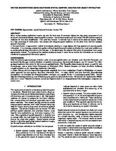
Figure 1. Global and regional context of the study area. Inset shows the location of Cerberus Fossae in relation to the InSight landing site. Main image shows the fault trace (red line) of the Cerberus Fossae system. Base image is a colorized Mars Orbiter Laser Altimeter image overlain on a THEMIS daytime infrared image. Location of the main study area (Figure 2) is shown by the black box and HiRISE stereo pairs by the white boxes.

that propagated through to final correlation and displacement results. In our case of searching for meterscale, fault-driven steps in the displacement maps, we found HiPRECISION data to be essential and therefore used them throughout. Although we made four DTMs, we were restricted to using just DTM1 as the elevation data set throughout for a number of reasons. The first is that image viewing geometry meant that the vertical precision of both DTM2 and DTM4 was sufficiently low that the final data product was noisy at the meter-scale, with occasional blunders. Although the overall vertical precision of DTM3 was good, the different viewing geometries meant that 42% of the DTM pixels were interpolated in SOCET SET, rather than being the result of true pixel matching, resulting in a noisy data set at the 10-m scale throughout. Therefore, we used DTM1 throughout our analysis due to its good vertical precision and relatively low noise (only 5% of pixels were interpolated) but discuss some of the implications of this approach in section 5. 2.2. Orthorectification and Correlation Between 45 and 73 tie points were selected between the first image (T0) and each image of the time series (Table S3). All tie points were placed in similar locations in all images, away from recognized aeolian features in case they were active. The accuracy of the tie points was optimized with COSI-Corr using an initial and final window size of 256 × 256 and 128 × 128 pixels, respectively. All images were orthorectified and mapprojected with COSI-Corr, using the optimized tie points, DTM1 and required ancillary data (camera and orbital geometries). For reasons outlined in section 4, all images in the time series were correlated using a sliding window of 64 × 32 pixels (16 × 8 m) and a step of four pixels (1 m). All images were correlated with the T0 image as a baseline, as cumulative changes maximize the chance of success in identifying any active tectonic processes.

3. Study Region: Cerberus Fossae Our choice of general study region was guided by geology and image availability. We aimed to choose an area that stood a good chance of showing evidence of coseismic deformation (e.g., Runyon et al., 2011) but had sufficient repeat image coverage to explore different methods of investigation. Given that one of the fundamental image constraints was a stereo HiRISE image pair for DTM production, we were limited to small parts of the Cerberus Fossae fault system (Figure 1)—at the time of writing, only 39 HiRISE stereo pairs intersected part of the mapped fault system. We narrowed our choice of region by concentrating on areas of

GRINDROD ET AL.

1883

Journal of Geophysical Research: Planets

10.1029/2018JE005649

Figure 2. Local context and image footprints of the local study area. (a) CTX image (G12_022809_1900_6m) orthorectified by a stereo CTX DTM showing the latitude and longitude of the study area of Cerberus Fossae. Black box shows the location of Figure 3. (b) Footprints of the 8 overlapping HiRISE images used in this study. (c) Location of the stereo HiRISE DTMs generated for this study. DTM1 is used throughout (see text for details). (d) Timing of the different images showing the local season at time of image acquisition. (e) Emission angle of each image, with relative image timing.

Cerberus Fossae found to have peaks in boulder size-frequency distribution, attributed to ground shaking during geologically recent marsquakes (Roberts et al., 2012). 3.1. Regional Setting The main study region is part of the central Cerberus Fossae fault system, centered around 9.9°N, 157.8°E (Figure 2). Cerberus Fossae is a single system at this location, approximately 1–1.5 km wide and 600 m deep. There is a smaller (up to ~100 m wide and 30 m deep) isolated fault to the north that is orthogonal to the main system, in addition to a 10-km-long linear feature interpreted as a poorly developed fault, which is about 40 km north of and parallel to the main system. Cerberus Fossae in this region cuts through Late Amazonian Volcanic Unit (lAv), with Amazonian and Hesperian Volcanic Unit (AHv) about 12 km to the north of the main system and Hesperian and Noachian Transition Unit about 40 km to the east (Tanaka et al., 2014). Although there are complicating factors when determining surface ages through crater size frequency analysis of small craters (e.g., McEwen et al., 2005), all studies agree that the faults in Cerberus Fossae cut through units that are very late Amazonian in age, with estimates ranging from a few million years (Berman & Hartmann, 2002; Burr et al., 2002; Hartmann & Berman, 2000) to several tens of millions of years (McEwen et al., 2005; Plescia, 2003). Similarly, the age of faults in Cerberus Fossae is uncertain due to unknown slip rates, but independent studies agree that the faults present today formed entirely after the youngest surface units had formed (Taylor et al., 2013; Vetterlein & Roberts, 2010) and could still be active today (Roberts et al., 2012). The study area therefore appears to have the youngest surface

GRINDROD ET AL.

1884

Journal of Geophysical Research: Planets

10.1029/2018JE005649

formation age in the region, in addition to showing evidence of geologically recent fault activity. The faults at Cerberus Fossae are likely tectonic graben (e.g., Taylor et al., 2013; Vetterlein & Roberts, 2010), with their lateral extent and association with pit chains providing evidence that dike emplacement is the predominant regional driving process (e.g., Wyrick et al., 2004). Regardless of the ultimate cause of subsidence, it is clear that the young age of the features offers a good first target for identifying active tectonic processes on Mars with this method. Although not the focus of this study, the HiRISE DTM produced shows some obvious channels originating from our local study area to the main Athabasca Valles to the southeast, in addition to local depressions surrounding the parallel fault to the north, and locally either side of the main system valley. 3.2. Local Setting Although we explore the application of COSI-Corr to the full HiRISE image data available, we concentrate some of our effort on a region that allowed the best exploration of possible coseismic deformation and optimal imaging conditions for the approach taken. This local study area is focused on an amphitheater-headed valley, approximately 650 × 900 m in size and up to 300 m in depth, which branches off from the main Cerberus valley in a SSE direction. It is unclear whether water originated directly from this smaller valley, as it lies several hundred meters to the east of the main fluvial channel that emanates from the Cerberus valley and sources Athabasca Valles to the southeast. Laterally continuous, horizontally stratified material occurs in two distinct layers in this area, similar to features at Hephaestus Fossae interpreted as representing a transition from bedrock (likely a lava flow) to regolith at this depth (Warner et al., 2017).

4. Results 4.1. Effect of Using HiPRECISION Data A comparison of east-west displacement results using PDS and HiPRECISION data is given in Figure 3. We used relative time step T1 to explore the effect, as the two images in this interval are a stereo pair, and thus any artifacts identified at this stage would propagate from the DTM production process. Although the ISIS preprocessing procedure includes radiometric calibration (“hical”), image column normalization (“cubenorm”), and equalization (“hiequal”), geometric distortions can still occur due to high-frequency spacecraft jitter. These distortions can create problems with stereo correlation and affect the quality of a stereoderived DTM and any subsequent displacement measurements. In the along-track direction, the dominant artifact is a 0.5- to 0.75-m amplitude periodic signal with a wavelength of ~0.75 km, which is due to spacecraft jitter, and similar to signals observed in SPOT (Satellite pour l’Observation de la Terre ), ASTER, and Quickbird images of Earth, and HiRISE images of Mars (Ayoub et al., 2008, July). In these cases, attitude effects such as jitter have been successfully removed in postprocessing by calculating the mean residual offset in the image column (e.g., Leprince, Ayoub, et al., 2007; Scherler et al., 2008). In the across-track direction, the use of PDS data can cause false east-west displacement steps of about 0.5 to 0.75 m, which are the result of misalignment between the different charge-coupled devices (CCDs) of the HiRISE instrument (Figures 3b and 3d). A similar effect has been observed in SPOT images of Earth (Leprince, Barbot, et al., 2007). The use of HiPRECISION data reduces these false displacement steps to less than 0.5 m. Any artifacts left in the across-track direction can be identified as linear features parallel to the along-track direction. Thus, any candidate marsquake signals that mimic these remaining artifacts must be treated with caution. However, our use of HiPRECISION data has effectively removed all attitude effects such as jitter, with no periodic signals evident above at most a 10-cm amplitude (Figures 3c and 3e). 4.2. Coregistration and Correlation We first explored the choice of correlation sliding window size in COSI-Corr for one time period (T5), as it determines the spatial resolution of any potential Marsquake offset field measured (Leprince, Barbot, et al., 2007). Figure 4 shows the effect of using four different initial and final sliding window sizes with a frequency correlation process (Leprince, Barbot, et al., 2007). In general, the larger the pixel size of the sliding windows, the lower the noise in the correlation result. At larger sliding windows, long wavelength noise due to camera distortion and artifacts are present (Figures 4a and 4b); at smaller sliding windows, although the long

GRINDROD ET AL.

1885

Journal of Geophysical Research: Planets

10.1029/2018JE005649

Figure 3. Comparison of Planetary Data System (PDS) and HiPRECISION results. (a) Image T1 (PSP_004283_1900) showing the study area and shadow conditions in the main fault system. (b) East-west component of the T1 correlation (64 × 32 sliding window) using PDS data. Charge-coupled device (CCD) array distortions are clear in the along-track direction as steps in the apparent displacement. Profile locations are shown by black lines. (c) East-west component of the T1 correlation (64 × 32 sliding window) using HiPRECISION data. There is a notable reduction of detector artifacts in the apparent displacement. Profile locations are shown by the gray lines. (d) Comparison of the across-track displacement with both PDS and HiPRECISION data. Large, meter-scale steps have been removed with HiPRECISION data, with maximum noise from sub-CCD image artifacts about 30 cm in magnitude. (e) Comparison of the along-track displacement with both PDS and HiPRECISION data. Spacecraft jitter creates periodic displacements with a wavelength and amplitude of about 0.7 km and 50 cm, respectively, with PDS data. The use of HiPRECISION data appears to largely remove this signal without further processing necessary and was used throughout this study.

wavelength noise is reduced, short wavelength noise increases (Figures 4c and 4d). We settled on a sliding window of 64 × 32 pixels as a compromise between the two levels of noise and used the following correlation settings in COSI-Corr for all time periods: correlator = frequency, window size initial = 64 pixels, window size final = 32 pixels, step = 4 pixels (1 m), robustness = 4, mask threshold = 0.9, resampling = 1. In experimenting with the correlation sliding window size, we made two main observations: (1) areas in shadow in one or both images produce erroneous displacements due to missing/poorer quality image data, and (2) only one displacement signal that could possibly be argued as being similar to what would be expected from a marsquake remained in all correlation tests and time periods. We also experimented with the use of a low-pass filter to remove both CCD and camera model artifacts, in addition to some noise. We used the T3 correlation results, with a full image average west-east displacement of 7 (±76 cm) and applied a low pass convolution filter with a kernel size of 49 (Figure 5). This procedure is a built-in function in COSI-Corr and has been used successfully in terrestrial studies (Hollingsworth et al., 2012). The resulting filtered correlation (Figure 5d) contains no visible CCD or camera model artifacts and has a reduced average west-east displacement of 2 (±41 cm). Detailed views of our case study region (Figures 5f and 5h) show that this filter choice leaves behind some topographic and shadow noise but also any GRINDROD ET AL.

1886

Journal of Geophysical Research: Planets

10.1029/2018JE005649

Figure 4. Comparison of choice of correlation sliding window size. (a) East-west component of the T5 correlation, using a correlation sliding window of 128 × 64 pixels. Some charge-coupled device (CCD) artifacts are present, but there is little short wavelength noise. (b) East-west component of the T5 correlation, using a correlation sliding window of 64 × 32 pixels. Some CCD artifacts are still present, but there is some short wavelength noise. (c) East-west component of the T5 correlation, using a correlation sliding window of 32 × 16 pixels. Reduced CCD artifacts are present, but there is an increasing amount of short wavelength noise and some topographic artifacts. (d) East-west component of the T5 correlation, using a correlation sliding window of 16 × 8 pixels. Almost no CCD artifacts are evident, but short wavelength noise and topographic artifacts dominate the signal. (e)–(h) Close-up of (a)–(d), respectively, showing the location of the focus of our study, with the location of Figure 6 shown by the black box.

possible displacement signatures at the length scale of interest. However, although the filter results are promising in future best practice studies, for this work we used unfiltered correlation results to gauge the overall performance of the method and to avoid the possible introduction of erroneous signals and/or removal of real signals. Misregistration of tie points can give some estimate of the accuracy of the subsequent orthorectification and is given in Figure 6a and Table S3. In all cases the average misregistration is less than a single pixel, with the best (T0) and worst (T7) cases being ~3 × 10 5 and 0.4 pixels, respectively, in the east-west directions. The mean (±standard deviation) misregistration in the east-west and north-south directions is 0.06 (±1.8) and 0.04 (±1.2) pixels, respectively. The mean misregistration of all images in all directions is 0.079 pixels, corresponding to approximately 1.6 cm. Therefore, given that the tie points were selected as having undergone no change, we can use this misregistration value as a guide to the effective minimum displacement that can be identified. Figures 6b to 6h show histograms of displacement for each entire image in the time series. In most cases, the mean displacement is close to zero, albeit with standard deviation values that are significant. The lowest standard deviation in displacement occurs in image T1, which could be the result of there being the smallest time gap between images. It could be argued that there is indeed an overall increase in standard deviation with increasing time between images. However, no filtering has been applied in any of the image correlation results in Figure 6, and therefore, overall displacement also includes poorly correlated areas such as shadowed regions. In the case of T1, limiting the values to those pixels with a signal-to-noise ratio of >0.99 GRINDROD ET AL.

1887

Journal of Geophysical Research: Planets

10.1029/2018JE005649

Figure 5. Example of low-pass filtering to remove image artifacts. (a) HiRISE base image T3 (ESP_022875_1900), with the black box showing the location of the local example study area. (b) Original east-west component of the T3 correlation, using a correlation sliding window of 64 × 32 pixels. Charge-coupled device (CCD) and camera model artifacts are present. (c) The low pass filter derived from (b), using a low pass convolution filter with a kernel size of 49, and adding 10% of the original image back in. (d) Output of subtracting the filter from the original image. No obvious CCD artifacts are observed, leaving topographic noise, in addition to the displacement signal of interest. (e)–(h) Close-up of (a)–(d), respectively, showing the location of the focus of our study.

reduces the mean and standard deviation displacement values by factors of approximately 50 and 5, respectively. However, given that most of our analysis was on a local case study example with limited shadows, we use the full nonfiltered correlation results except where explicitly stated. 4.3. Local Case Study Example Our focus in searching for evidence of active coseismic deformation was concentrated on a single area and signal that could be argued to be most similar to that of a terrestrial earthquake (Figure 7). No other area in any image showed any such signal. The main pattern that we used to identify such a feature was an area with apparent displacement that was approximately equal in magnitude, but opposite in direction, either side of a linear feature that could be a fault. Numerous examples of this sort of earthquake feature have been identified in terrestrial studies using COSI-Corr (e.g., Avouac et al., 2006; Copley et al., 2011; Hollingsworth et al., 2012, 2017; Konca et al., 2010; Kuo et al., 2014; Leprince, Barbot, et al., 2007) and compared to similar processes identified with interferometric synthetic aperture radar data (e.g., Jonsson et al., 2003; Simons et al., 2002). Figure 7 shows detailed views of the correlation results for our local case study example. The case study area lies on steep southwest facing slopes that run down from relatively flat plains. Only one obvious DTM error, away from the signal of interest, is obvious in this area and was avoided in all measurements. Correlation results from images T1 and T2 are relatively noisy, but images T3 and T4 show near identical results of up to 1–2 m west displacement near the top of the slope and up to 1–2 m of east displacement lower down the slope. Images T5 and T6 show almost identical displacement results but with the directions reversed. Image T7 is again too noisy to interpret with confidence. No other displacement signals in any image in this local area demonstrated such a distinct and consistent, albeit reversing, signature. The

GRINDROD ET AL.

1888

Journal of Geophysical Research: Planets

10.1029/2018JE005649

Figure 6. Summary of the misregistration and displacement of each relative image timing. (a) The mean (vertical black line) and one standard deviation (box) of the east-west (red) and north-south (gray) components of the correlation (64 × 32 pixel sliding window) for each relative image. T0 represents the base image (PSP_003650_1900) coregistered and orthorectified to its own SOCET SET image but with a stereo DTM and shows the lowest misregistration. (b)–(h) Histograms of the east-west and north-south displacements across the whole of images T1 to T7, respectively. Also given in each case is the mean and standard deviation.

profiles through the local area (Figure 8) show these correlation results in a different manner. The shape of the surface in the profile region is given in Figure 8a, with west-east displacements for all images in the time series in subsequent subfigures. Again, correlation results from images T1 and T2 are relatively noisy and show no definite trend. However, images T3 and T4 highlight the possible displacement pattern, with between 1- and 2-m displacement in opposite directions, over a length scale of about 40 m. This trend continues, but in the opposite direction, in images T5 and T6, with image T7 too noisy to see any definite trend. To further investigate whether the displacement trends seen in the local case study are indeed real, we calculated the displacement vectors in the best case result, image T4 (Figure 9a). These vectors show that the apparent displacement corresponds with the base (easterly movement) and top (westerly movement) of a steep slope, with both signals concentrated on two subhorizontal layers separated by likely scree material. Therefore, the possibility of having found evidence of coseismic deformation is not immediately ruled out by the local geology that corresponds to the displacement signals. Instead, as none of the images in the time series are nadir looking, we expect parallax difference between images if topography is not entirely corrected during the orthorectification stage. To overcome this problem, previous studies have reprojected images and correlation results into the epipolar and epipolar perpendicular planes (e.g., Hollingsworth et al., 2012). In this projection, the topographic noise should be isolated to the epipolar plane displacement field. We follow the same technique by using the “Epipolar Map Projection” tool in COSI-Corr and investigate the epipolar perpendicular plane, as it should contain no topographic

GRINDROD ET AL.

1889

Journal of Geophysical Research: Planets

10.1029/2018JE005649

Figure 7. Example of local displacement results. (a)–(h) HiRISE images T0 to T7 respectively. (i) Stereo DTM1 overlain on a hillshade image. Contours represent 100(thick lines) and 10-m (thin lines) intervals. Black arrow shows the location of a small DTM blunder. (j)–(p) East-west component of the correlation (64 × 32 sliding window) for images T1 to T7, respectively. In each case the location of the stacked profiles (average of 10 profiles 1 pixel apart) given in Figure 8 is shown. Grid spacing is 10 m.

information. Figure 9b shows the epipolar perpendicular correlation results, which do not contain any displacements that can confidently be attributed to coseismic deformation. Therefore, rather importantly, removing the effect of topography also removes any possible signal of a Marsquake, thus making it unlikely that we have observed active deformation due to a seismic event. 4.4. Ancillary Observations Although it is unlikely that we have found evidence of a coseismic event, the production of images that are coregistered and orthorectified to a high level of precision means that ancillary observations can be made to support or refute the main finding. In this case, we mapped all dark streaks that resembled recurring slope lineae (RSLs; McEwen et al., 2011) in all images in the time series. Given that RSLs are thought to be the result of seasonal processes, growing in length in summer and fading or disappearing entirely in winter (e.g., Chojnacki et al., 2016; McEwen et al., 2011, 2014), any deviation from this trend could be the result of stochastic timing triggered by seismic activity. Figure 10 shows the location, density, and length statistics for

GRINDROD ET AL.

1890

Journal of Geophysical Research: Planets

10.1029/2018JE005649

Figure 8. Example of 50 pixel-wide stacked profiles over example study region. (a) Plots of the elevation and derived slope from DTM1. (b)–(h) Plots of the east-west component of the correlation (64 × 32 sliding window) for images T1 to T7, respectively. Both the mean (black line) and one standard deviation (gray region) is given in each case. T1 and T2 are too noisy to interpret, but images T3–T6 are similar to a typical displacement plot across a fault, with the order of 1 m throw over a baseline of about 50 m, albeit with a reversal in direction between T4 and T5. Image T7 has increased noise but appears to continue the same trend. Vertical dotted and dashed lines in each case represent the location of the extent and peak displacement, respectively, in T4.

candidate RSLs in each image along the main Cerberus Fossae wall slopes. Almost all identified candidate RSLs occur on south-facing slopes, with some also occurring on west-facing slopes in our local case study region. Through the time series from T0 to T7, the number of individual RSL-like features was 50, 45, 21, 88, 46, 6, 6, and 1 respectively. However, the number of RSLs does not correspond with the length, with the respective mean lengths being 28, 36, 43, 28, 36, 30 26, and 23 m. There is a marked increase in the number of RSLs in image T3, which was taken in northern hemisphere winter only 5 sols after image T2 and corresponds to when the possible displacement is first observed with confidence in the case study area. In image T4, taken 135 sols later and in northern hemisphere spring, the number of RSLs has almost halved, but the mean length has increased from 28 to 36 m. Almost all RSL candidates are not evident by image T5, when a reversal in the displacement signal was observed and continue to be absent in T6 and T7.

Figure 9. Epipolar perpendicular displacement. (a) West-east component of the T4 correlation, using a correlation sliding window of 128 × 64 pixels. Purple arrows show the displacement direction and magnitude of this result. (b) Reprojection of the displacement map in (a) into the epipolar perpendicular plane. Black arrows show the direction of this plane across the image, which are parallel due to the consistent use of pushbroom detector images before and after the possible event (c.f. Hollingsworth et al., 2012). Any possible marsquake signal is eliminated in this projection.

GRINDROD ET AL.

1891

Journal of Geophysical Research: Planets

10.1029/2018JE005649

Figure 10. Recurring slope lineae (RSLs) distribution over time in the study area. (a)–(h) shows the location (black lines) and density (color scale) of RSLs in this part of Cerberus Fossae for each relative image timing. Box and whisker plots in each case show the length of the RSLs at each time through the following measurements: median (red line), the 25th and 75th centile (blue box), range (whiskers), and outliers (1.5 times the interquartile range away, red dots).

Several candidate RSLs and other dark slope features were observed to grow and fade in our local case study area (Figure 11). No RSLs or other dark slope features were observed until T2, when a 95-m RSL, partially bifurcated, appeared ~200 m to the south of the possible displacement signatures, originating from the second subhorizontal layer and flowing down a scree surface. This RSL has shrunk to 91 m by T3, but a second shorter RSL has appeared, originating from the first subhorizontal layer. This small RSL has faded by T4, with no change in the long RSL, but there is an apparent darkening of material ~160 m to the west of the possible

GRINDROD ET AL.

1892

Journal of Geophysical Research: Planets

10.1029/2018JE005649

Figure 11. Recurring slope lineae (RSLs) over time in the local example study area. (a)–(h) show the same location with the relative image in the background and RSLs marked by the red lines and black arrows. The length of the dominant RSL is given in each case when present. The red arrows highlight non-RSL features that appear to have darkened in that relative image.

displacement signatures. RSLs remain essentially unchanged in T5, although the large dark material has faded to previous levels. In T6 the main RSL has started to appear to break up through fading at different parts of the length, but there is also a subtle dark feature that runs below and almost parallel to the second subhorizontal layer that is not present in any other image. By T7, all RSLs and associated dark features have faded in the local case study area. We acknowledge that apparent fading of these dark features can be misleading, and so according to a rigorous definition (McEwen et al., 2014), our RSLs are only partially confirmed.

5. Discussion We break down the discussion of our results into three main sections covering (1) investigating a localized and large amplitude signal, (2) predictions of what fault events should be detectable with different detectors, and (3) recommendations for future use of the method in seismic applications. 5.1. Localized Large Amplitude Signal One of the ultimate goals of this study was to identify any evidence of surface deformation associated with marsquakes. Although we did not see such evidence, we did identify some systematic signals with large amplitude that are inconsistent with earthquakes but remain unaccounted for. We need to better understand the source of these signals to establish if they are (1) noise introduced by the data or the processing or (2) real signals from some yet unknown or poorly understood process (e.g., mass wasting). Given that we do not currently know the state of seismic activity on Mars, it is necessary to first look at the dynamics that would be associated with any fault that could have produced the signal and, second, the data used in the analysis. The former will provide information on whether any possible displacement of the type observed is likely from a geologic perspective, whereas the latter can help us determine whether any possible displacement is the result of artifacts of the data or processing. The consensus view is that Cerberus Fossae fault system is a large tectonic feature made up of many individual normal faults or fault-controlled pits in association with dike emplacement and volcanism (e.g., Ernst et al., 2001; Head et al., 2003; Plescia, 2003; Taylor et al., 2013; Vetterlein & Roberts, 2010). Previous estimates of the maximum fault throw measured at the main fault system studied here range from approximately 600 (Taylor et al., 2013) to 2,000 m (Vetterlein & Roberts, 2010), demonstrating significant slip on any normal faults responsible. Our best (and only) correlation result that resembles terrestrial earthquake displacement

GRINDROD ET AL.

1893

Journal of Geophysical Research: Planets

10.1029/2018JE005649

suggests that 1–2 m of west-east displacement (Dmax) has occurred, possibly twice in opposite directions, over a length scale (L) of about 50 m, giving Dmax/L values of 0.02 to 0.04, respectively. Extensive study has shown that there is significant variation in the displacement-length scaling of all types of terrestrial faults, due to a combination of fault mechanics and measurement techniques (e.g., Kim & Sanderson, 2005; Scholz, 2002). Nonetheless, our possible fault-displacement characteristics are not unrealistic and lie toward the middle to upper end of typical Dmax/L values for normal faults (e.g., Cowie & Scholz, 1992a, 1992b; Dawers et al., 1993; Kim & Sanderson, 2005). However, simple analysis of the stress that would occur on this system refutes the idea of active faulting in this local case study. To estimate the seismic moment (M) expected, we can use the simplified relationship M = μAD, where μ is the shear modulus, A is the fault rupture area, and D is the displacement. Using our above values, and an assumed shear modulus of 30 GPa (e.g., Scholz, 2002), gives values of M of between 2.5 × 1014 and 5 × 1014 Nm. From studies of the Earth (Kanamori & Anderson, 1975), we can also use the approximation M = ΔσA3/2, where Δσ is the static stress drop. Rearranging the above equation allows us to estimate the stress drop of a feature of the size we have identified as between 2,000 and 4,000 MPa. Although the stress-drop is scale-independent, typical earthquake stress drop values are between 1 and 10 MPa (e.g., Scholz, 2002). In short, any fault at this location would have activated long before the stresses reached such high values and implies that the possible fault dynamics are implausible. In addition, the small spatial extent and decay wavelength would suggest that any marsquake here nucleated in the shallowest part of the crust, which is unlikely given the low normal stresses expected at these depths and perhaps supports Cerberus Fossae being the result of collapse atop dilational faults at depth (Runyon et al., 2011; Wyrick et al., 2004). Although it is not possible to confidently predict the nature of any possible fault in our local case study area due to the resolution of the topographic data being too poor, it is possible that if present, any fault is not a simple, single normal fault. Instead, the presence of two distinct layers in the wall and the possible displacement pattern could suggest a number of possible different fault type and geometries, including an obliqueslip or double fault. It is also possible that any possible activation and reversal in displacement direction in our local case study area could be the result of a change in the larger stress conditions, as experienced, for example, by the propagation of a dike and the evolution of a stress shadow (e.g., Green et al., 2015). Overall, although the fault-displacement characteristics and possible geometries are not unrealistic compared to terrestrial faults, the stress analyses and epipolar perpendicular correlation results strongly suggest that topography was not entirely corrected during the orthorectification stage and that we have not observed coseismic displacement in this case. This interpretation is supported by the observation parameters of the images in the time series. The apparent reversal in the possible displacement signal occurs in images T5 and T6, the only images that have an emission angle lower than the base image T0 (Figure 12). In effect, the topographic effect in the correlation results is likely a result of the near-nadir observations containing few to no pixels covering the steep (>80°) slopes of the canyon walls. Although there will be an element of observational bias due to image properties and season, we also see no definitive evidence in the distribution and timing of candidate RSLs to support their formation through coseismic deformation that matches the timing observed in our correlation results. However, the sudden increase in RSL-like features between images T2 and T3, which were also taken under similar conditions, is an interesting observation that does not easily sit with the hypothesis that liquid water, albeit a brine, is responsible (McEwen et al., 2011; Ojha et al., 2015) for their formation and aligns better with water-free formation mechanisms (Dundas et al., 2017). 5.2. Prediction of Detectability Given prior COSI-Corr performance (e.g., Leprince, Barbot, et al., 2007), it should be possible to identify coseismic displacements in HiRISE images at the centimeter-scale. Although there are possible complicating factors when determining surface ages through crater size frequency analysis of small craters (McEwen et al., 2005), all studies agree that the faults and/or pits in Cerberus Fossae cut through units that are very late Amazonian in age, with estimates ranging from a few million years (Berman & Hartmann, 2002; Burr et al., 2002; Hartmann & Berman, 2000) to several tens of millions of years (McEwen et al., 2005; Plescia, 2003). We can use these maximum ages to predict the likely slip rates and thus whether the displacement is observable with COSICorr using two end-member cases: (1) fault creep and (2) fault stick-slip.

GRINDROD ET AL.

1894

Journal of Geophysical Research: Planets

10.1029/2018JE005649

Figure 12. Summary of image observation geometry. (a) East-west component of the T4 correlation, using a correlation sliding window of 64 × 32 pixels. Stereo DTM1 contours represent 100- (thick lines) and 10-m (thin lines) intervals. Thick dashed line shows the approximate location of the boundary between the zones of equal and opposite displacement. (b) Aspect of the surface from DTM1. (c) Slope map of DTM1 scaled to emphasize steep regions. The study area has slopes greater than 80° in places. (d) Fig. of Merit (FOM) values of DTM1 in the local study area. Values 40 actually representing successful automatic correlation in SOCET-SET. (e) Schematic diagram showing the observation geometry of the different relative image timings. T0 is the base image and is shown in each case for comparison. In images T5 and T6 the emission angle is less than that of T0, essentially leading to a different look direction.

5.2.1. Fault Creep The characteristic earthquake model states that individual faults and fault segments in a single fault zone generate earthquakes of essentially the same magnitude (e.g., Schwartz & Coppersmith, 1984), resulting in a constant slip rate over time when averaged. Active normal faults in terrestrial rift basins on Earth have slip rates of 0.01–10 mm/year (e.g., Cowie & Roberts, 2001). Over an assumed 15-year period, successful HiRISE image correlations with COSI-Corr of 1/20 and 1/50 pixels could detect minimum slip rates of 0.75 and 0.3 mm/year, respectively (Figure 13), well within terrestrial rates. The slip rate on faults at Cerberus Fossae are poorly constrained due to the uncertainty in their age, but if any faulting occurred in the last 850 ka at faults with all but the smallest throws, then our technique should be capable of detecting the movement, regardless of the slip rate (Figure 13). Similar predictions for CTX and CaSSIS images at 1/50 pixel correlation yield detectable slip rates of 8 and 6 mm/year, respectively. A caveat to this estimate is that any signal would be best observed by our method if the fault was creeping at the surface; if creep was occurring on part of a fault at depth, the signal would be filtered by the overlying elastic crust producing a longwavelength arctan-like signal, with the resultant change of signal more difficult to detect with these optical methods. 5.2.2. Fault Stick-Slip The modified overlap model of earthquakes states that small portions of a fault can rupture with variations in time and location (Roberts, 1996), resulting in regions with relatively short earthquake recurrence intervals. There is recent, tantalizing evidence of extremely recent marsquakes at faults in Cerberus Fossae, from the spatial variation in boulder size populations along the graben (Roberts et al., 2012). The boulders have left trails in aeolian ripples, which can be used to estimate the timing of the marsquake(s) possibly responsible for triggering boulder avalanches. Recent work using COSI-Corr has derived ripple migration rates of 0.2–1 m/year on Mars (Bridges et al., 2012), implying that a 1-m-wide boulder track (i.e., 4 HiRISE pixels to be resolvable) would be obscured by active ripple movement at the bottom of Cerberus Fossae in 1–50 years. Assuming a 1/20 pixel correlation with COSI-Corr means that new boulders and/or boulder trails of 0.0125, 0.3, and 0.23 m in size could be identified with our technique with HiRISE, CTX or CaSSIS data, respectively. The above analysis is based on the assumption that ripple movement occurs at similar rates across Mars.

GRINDROD ET AL.

1895

Journal of Geophysical Research: Planets

10.1029/2018JE005649

Figure 13. Prediction of detectability of coseismic displacements with COSI-Corr. In each case solid gray lines show theoretical fault slip rates as a function of maximum throw on individual faults and time since faulting. Terrestrial data are from onshore and offshore fault systems. Mars data are from two different sources: Four faults at Cerberus Fossae, with maximum ages of 2.5 Ma; four faults with variable maximum ages. In both Mars cases, the maximum age is an estimate due to the inherent problems with crater counting of very young surfaces, whereas the minimum age is essentially unconstrained. Shaded gray regions show the detectability ranges for the COSI-Corr method at both 0.05 (1/20) and 0.02 (1/50) pixel correlations. Predictions are made for (a) High-Resolution Imaging Science Experiment (HiRISE), (b) Context Camera (CTX), and (c) Color and Stereo Surface Imaging System (CaSSIS) imaging instruments. (d) shows the post-priori correlation performance for each image.

Further analysis is needed for studying any movement of the ripples in Cerberus Fossae, which is optimized for aeolian features and takes into account the detrimental effect of shadows. The identification of no coseismic displacement or related features will still provide important results, as the threshold detection limit for the COSI-Corr method and image data will be used to determine for the first time a definitive maximum current slip rate. This slip rate can then be used to calculate the cumulative total moment release on the faults, which has been used to predict the size-frequency distribution of seismic events on Mars (Knapmeyer et al., 2006; Taylor et al., 2013). To this end we can determine our correlation performance post-priori in this study, for comparison with the predictions of detectability (Figure 13d). Our best

GRINDROD ET AL.

1896

Journal of Geophysical Research: Planets

10.1029/2018JE005649

performing image in terms of coregistration was T0, as it was tied to itself and therefore should not be used to test performance. Instead, the average coregistration performance of each image in this study suggests that fault slip rates of between 0.1 and almost 10 mm/year should be detectable using this method (Figure 13d). If correct, our results suggest that there has been no seismic movement in the study area during the interval of HiRISE imaging at these orders of magnitude scales. 5.3. Recommendations for Future Use Although previous studies have used COSI-Corr in studies of aeolian features on Mars (Ayoub et al., 2014; Bridges et al., 2012; Cardinale et al., 2016; Runyon et al., 2017; Silvestro et al., 2016), this study is the first attempt to use this method for identifying and quantifying coseismic displacement. Even though it is unlikely that we have successfully identified a marsquake, we can offer recommendations for future use of the method to maximize the chance of success. In terms of image acquisition, given that we need a highresolution DTM, then there needs to be a stereo pair with little time gap between images to minimize the chance of any changes affecting the quality of the resulting DTM. Then just one other image taken either before or after the DTM is required, with as much time gap as possible to maximize the chance of identifying coseismic displacement. In addition, to minimize any possible topographic effects in the correlation results, the third image should be taken with observation parameters as close as possible, preferably identical, to one of the stereo pair images that will be used for correlation. Returning repeat HiRISE or CTX images of an area with these image constraints is a difficult and data-heavy procedure. However, the CaSSIS imaging instrument on the ExoMars 2016 TGO is particularly well suited to this task, as it is designed to acquire a stereo pair for DTM production on a single orbit. Single HiRISE or CTX images can then be used as the third image in the sequence, taken before CaSSIS images were acquired and giving a time gap of up to 14 years at the start of TGO science operations. Given that no previous studies have investigated the use of CTX data with COSI-Corr, which can also be used as a proxy for CaSSIS image resolution and coverage, our current focus is on quantifying the changes, both coseismic and eolian, that can be identified and quantified with these data. Initial results are promising and will be published in a future study. Once images have been acquired and correlations have been determined, then there are several different approaches that could be used in future studies to improve the results. A more rigorous assessment and removal of DTM errors and topographic effects could be explored in future studies, in an attempt to identify subtle changes (Scherler et al., 2008). The use of post-processing filters could also be investigated, with direction and magnitude having been successfully used with terrestrial data to improve the correlation results (e.g., Scherler et al., 2008) and median filters used to remove high-frequency noise (Hollingsworth et al., 2012; Hollingsworth et al., 2013). Principal component analysis has also been used with correlation results for Mars (Ayoub et al., 2014) and could be tested in future tectonic studies. Given that the method used here is a time- and data-heavy procedure, it is useful to target areas with the best chance of having undergone recent, or even active, seismic activity. We used a previous study of boulder distribution in Cerberus Fossae to guide our selection of study area (Roberts et al., 2012), but future studies could use the detection of possible diagnostic fault-related mineralogies (e.g., Arancibia et al., 2014; Sánchez-Roa et al., 2017) as a proxy for age, as presumably older fault surfaces will either be masked by dust or collapse scree. If internal cooling and large lithospheric loads are the dominant source of seismicity (e.g., Panning et al., 2016), then studies of faults near the Tharsis region would be useful. Finally, direct detection of seismic activity by the InSight mission could yield a marsquake location (Böse et al., 2017), faults within which could then be studied with COSI-Corr to provide independent confirmation and complementary information on martian seismicity.

6. Conclusions We have conducted the first search for active seismic activity on Mars using subpixel image coregistration and correlation. Our study focused on one area of the Cerberus Fossae fault system, to the southeast of the Elysium volcanic province. We used eight overlapping HiRISE images taken over a time period of about 8.5 Earth years in an attempt to identify and quantify any surface changes that could be attributable to seismic displacement. In using this approach, it is evident that unless suitable postprocessing techniques are developed, the use of jitter-corrected images significantly improves the correlation results. Investigation of the correlation parameters highlighted the different scale of image noise and possible changes in the

GRINDROD ET AL.

1897

Journal of Geophysical Research: Planets

10.1029/2018JE005649

resultant displacement maps, which can be improved with the use of a low-pass filter postprocessing. Together with the use of jitter-corrected images, this filtering can effectively remove almost all instrument artifacts from the final correlation data. Overall, we saw no strong evidence for coseismic displacement in our study region during the time period of the observations. One candidate signal had some similarities with typical terrestrial earthquake displacement, with an apparent west-east displacement of 1–2 m, possibly twice in opposite directions, over a length scale of about 50 m. This signal was present, albeit with different noise levels, in all of the images in the time series. However, we dismissed this signal as evidence of coseismic deformation and, through the use of an epipolar perpendicular projection, instead interpreted this signal to be the result of the incomplete correction of topography during the coregistration stage. Ancillary observations of RSL activity in the surrounding fault system, which could be triggered by stochastic seismic events, do not obviously support the observation of a seismic event, although RSL activity that does not match previous seasonal observations elsewhere requires further explanation. Nonetheless, our study offers a best practice approach in searching for active marsquakes with orbital images, which can be used to complement and independently verify in situ observations by the InSight lander. Acknowledgments The standard data used in this study are available at the NASA PDS Imaging Node, Mars Reconnaissance Orbiter Online Data Volumes (https://pdsimaging.jpl.nasa.gov/volumes/mro. html), the stereo DTM at Figshare (doi: 10.6084/m9.figshare.6384035), and all HiPRECISION image data at Figshare (doi: 10.6084/m9.figshare.6383834). P. M.G. was supported by the UK Space Agency (grants ST/J002127/1, ST/J005215/1, ST/L00254X/1, and ST/R002355/1). S.H. was supported by NERC (grants NE/L006898/1 and NE/P017525/1). The stereo DTM processing was carried out at the Natural History Museum, London. This work has benefited from discussions with Pieter Vermeesch, Joel Davis, Gerald Roberts, and Matt Balme. We thank Sarah Sutton, Audrie Fennema, and the HiRISE team for the production of HiPRECISION data products. We also thank the United States Geological Survey Astrogeology Mapping, Remote-sensing, Cartography, Technology, and Research (MRCTR) Geographical Information System Lab for ongoing support with producing stereo DTMs. We thank Kirby Runyon and an anonymous reviewer for helpful comments that improved the quality of this paper.

GRINDROD ET AL.

References Anderson, D. L., Kovach, R. L., Latham, G., Press, F., Nafi Toksoz, M., & Sutton, G. (1972). Seismic investigations: The Viking Mars Lander. Icarus, 16(1), 205–216. https://doi.org/10.1016/0019-1035(72)90147-9 Anderson, D. L., Miller, W. F., Latham, G. V., Nakamura, Y., Toksöz, M. N., Dainty, A. M., et al. (1977). Seismology on Mars. Journal of Geophysical Research, 82(28), 4524–4546. https://doi.org/10.1029/JS082i028p04524 Arancibia, G., Fujita, K., Hoshino, K., Mitchell, T. M., Cembrano, J., Gomila, R., et al. (2014). Hydrothermal alteration in an exhumed crustal fault zone: Testing geochemical mobility in the Caleta Coloso Fault, Atacama Fault System, Northern Chile. Tectonophysics, 623, 147–168. https://doi.org/10.1016/j.tecto.2014.03.024 Avouac, J.-P., Ayoub, F., Leprince, S., Konca, O., & Helmberger, D. V. (2006). The 2005, Mw 7.6 Kashmir earthquake: Sub-pixel correlation of ASTER images and seismic waveforms analysis. Earth and Planetary Science Letters, 249(3), 514–528. https://doi.org/10.1016/j. epsl.2006.06.025 Ayoub, F., Avouac, J. P., Newman, C. E., Richardson, M. I., Lucas, A., Leprince, S., & Bridges, N. T. (2014). Threshold for sand mobility on Mars calibrated from seasonal variations of sand flux. Nature Communications, 5(1), 5096. https://doi.org/10.1038/ncomms6096 Ayoub, F., Leprince, S., Binet, R., Lewis, K. W., Aharonson, O., & Avouac, J. P. (2008, July). Influence of camera distortions on satellite image registration and change detection applications. Paper presented at 2008 IEEE International Geoscience and Remote Sensing Symposium, IGARSS 2008, IEEE, Piscataway, NJ. Banerdt, W. B., Smrekar, S., Hurst, K., Lognonné, P., Spohn, T., Asmar, S., et al. (2013). InSight: A discovery mission to explore the interior of Mars. Paper (#1915) presented at 44th Lunar and Planetary Science Conference, The Woodlands, TX, edited. Berman, D. C., & Hartmann, W. K. (2002). Recent fluvial, volcanic, and tectonic activity on the Cerberus Plains of Mars. Icarus, 159(1), 1–17. https://doi.org/10.1006/icar.2002.6920 Böse, M., Clinton, J. F., Ceylan, S., Euchner, F., van Driel, M., Khan, A., et al. (2017). A probabilistic framework for single-station location of seismicity on Earth and Mars. Physics of the Earth and Planetary Interiors, 262, 48–65. https://doi.org/10.1016/j.pepi.2016.11.003 Bridges, N. T., Ayoub, F., Avouac, J. P., Leprince, S., Lucas, A., & Mattson, S. (2012). Earth-like sand fluxes on Mars. Nature, 485(7398), 339–342. https://doi.org/10.1038/nature11022 Burr, D. M., Grier, J. A., McEwen, A. S., & Keszthelyi, L. P. (2002). Repeated aqueous flooding from the Cerberus Fossae: Evidence for very recently extant, deep groundwater on Mars. Icarus, 159(1), 53–73. https://doi.org/10.1006/icar.2002.6921 Cardinale, M., Silvestro, S., Vaz, D. A., Michaels, T., Bourke, M. C., Komatsu, G., & Marinangeli, L. (2016). Present-day aeolian activity in Herschel crater, Mars. Icarus, 265, 139–148. https://doi.org/10.1016/j.icarus.2015.10.022 Chojnacki, M., McEwen, A., Dundas, C., Ojha, L., Urso, A., & Sutton, S. (2016). Geologic context of recurring slope lineae in Melas and Coprates Chasmata, Mars. Journal of Geophysical Research: Planets, 121, 1204–1231. https://doi.org/10.1002/2015JE004991 Copley, A., Avouac, J.-P., Hollingsworth, J., & Leprince, S. (2011). The 2001 Mw 7.6 Bhuj earthquake, low fault friction, and the crustal support of plate driving forces in India. Journal of Geophysical Research, 116, B08405. https://doi.org/10.1029/2010JB008137 Cowie, P. A., & Roberts, G. P. (2001). Constraining slip rates and spacings for active normal faults. Journal of Structural Geology, 23(12), 1901–1915. https://doi.org/10.1016/S0191-8141(01)00036-0 Cowie, P. A., & Scholz, C. H. (1992a). Growth of faults by accumulation of seismic slip. Journal of Geophysical Research, 97(B7), 11,085–11,095. https://doi.org/10.1029/92JB00586 Cowie, P. A., & Scholz, C. H. (1992b). Physical explanation for the displacement-length relationship of faults using a post-yield fracture mechanics model. Journal of Structural Geology, 14(10), 1133–1148. https://doi.org/10.1016/0191-8141 (92)90065-5 Dandonneau, P.-A., Lognonné, P., Banerdt, W. B., Deraucourt, S., Gabsi, T., Gagnepain-Beyneix, J., et al. (2013). The SEIS InSight VBB experiment. Paper (#2006) presented at 44th Lunar and Planetary Science Conference, Lunar and Planetary Institute, Houston, TX. Dawers, N., Anders, M. H., & Scholz, C. (1993). Growth of normal faults: Displacement-length scaling. Geology, 21(12), 1107–1110. https://doi. org/10.1130/0091-7613(1993)0212.3.CO;2 Dundas, C. M., McEwen, A. S., Chojnacki, M., Milazzo, M. P., Byrne, S., McElwaine, J. N., & Urso, A. (2017). Granular flows at recurring slope lineae on Mars indicate a limited role for liquid water. Nature Geoscience, 10(12), 903–907. https://doi.org/10.1038/s41561-017-0012-5 Ernst, R., Grosfils, E., & Mège, D. (2001). Giant dike swarms: Earth, Venus, and Mars. Annual Review of Earth and Planetary Sciences, 29(1), 489–534. https://doi.org/10.1146/annurev.earth.29.1.489 Golombek, M. (2002). A revision of Mars seismicity fromsurface faulting. Paper (#1244) presented at 33rd Lunar and Planetary Science Conference, Lunar and Planetary Institute, Houston, TX. Golombek, M. P., Banerdt, W. B., Tanaka, K. L., & Tralli, D. M. (1992). A prediction of Mars seismicity from surface faulting. Science, 258(5084), 979–981. https://doi.org/10.1126/science.258.5084.979 Green, R. G., Greenfield, T., & White, R. S. (2015). Triggered earthquakes suppressed by an evolving stress shadow from a propagating dyke. Nature Geoscience, 8(8), 629–632. https://doi.org/10.1038/ngeo2491

1898

Journal of Geophysical Research: Planets

10.1029/2018JE005649

Hartmann, W. K., & Berman, D. C. (2000). Elysium Planitia lava flows: Crater count chronology and geological implications. Journal of Geophysical Research, 105(E6), 15,011–15,025. https://doi.org/10.1029/1999JE001189 Head, J. W., Wilson, L., & Mitchell, K. L. (2003). Generation of recent massive water floods at Cerberus Fossae, Mars by dike emplacement, cryospheric cracking, and confined aquifer groundwater release. Geophysical Research Letters, 30(11), 1577. https://doi.org/10.1029/ 2003GL017135 Herman, F., Anderson, B., & Leprince, S. (2011). Mountain glacier velocity variation during a retreat/advance cycle quantified using sub-pixel analysis of ASTER images. Journal of Glaciology, 57(202), 197–207. https://doi.org/10.3189/002214311796405942 Hollingsworth, J., Leprince, S., Ayoub, F., & Avouac, J.-P. (2012). Deformation during the 1975–1984 Krafla rifting crisis, NE Iceland, measured from historical optical imagery. Journal of Geophysical Research, 117, B11407. https://doi.org/10.1029/2012JB009140 Hollingsworth, J., Leprince, S., Ayoub, F., & Avouac, J.-P. (2013). New constraints on dike injection and fault slip during the 1975–1984 Krafla rift crisis, NE Iceland. Journal of Geophysical Research: Solid Earth, 118, 3707–3727. https://doi.org/10.1002/jgrb.50223 Hollingsworth, J., Ye, L., & Avouac, J.-P. (2017). Dynamically triggered slip on a splay fault in the Mw 7.8, 2016 Kaikoura (New Zealand) earthquake. Geophysical Research Letters, 44, 3517–3525. https://doi.org/10.1002/2016GL072228 Jonsson, S., Segall, P., Pedersen, R., & Bjornsson, G. (2003). Post-earthquake ground movements correlated to pore-pressure transients. Nature, 424(6945), 179–183. https://doi.org/10.1038/nature01776 Kanamori, H., & Anderson, D. L. (1975). Theoretical basis of some empirical relations in seismology. Bulletin of the Seismological Society of America, 65(5), 1073–1095. Kim, Y.-S., & Sanderson, D. (2005). The relationship between displacement and length of faults: A review. Earth Science Reviews, 68(3–4), 317–334. https://doi.org/10.1016/j.earscirev.2004.06.003 Kirk, R. L. (2003). High-resolution topomapping of candidate MER landing sites with Mars Orbiter Camera narrow-angle images. Journal of Geophysical Research, 108(E12), 8088. https://doi.org/10.1029/2003je002131 Kirk, R. L., Howington-Kraus, E., Rosiek, M. R., Anderson, J. A., Archinal, B. A., Becker, K. J., et al. (2008). Ultrahigh resolution topographic mapping of Mars with MRO HiRISE stereo images: Meter-scale slopes of candidate Phoenix landing sites. Journal of Geophysical Research, 113, E00A24. https://doi.org/10.1029/2007je003000 Knapmeyer, M., Oberst, J., Hauber, E., Wählisch, M., Deuchler, C., & Wagner, R. (2006). Working models for spatial distribution and level of Mars’ seismicity. Journal of Geophysical Research, 111, E11006. https://doi.org/10.1029/2006JE002708 Konca, A. O., Leprince, S., Avouac, J.-P., & Helmberger, D. V. (2010). Rupture process of the 1999 Mw 7.1 Duzce earthquake from joint analysis of SPOT, GPS, InSAR, Strong-Motion, and Teleseismic data: A Supershear rupture with variable rupture velocity. Bulletin of the Seismological Society of America, 100(1), 267–288. https://doi.org/10.1785/0120090072 Kuo, Y.-T., Ayoub, F., Leprince, S., Chen, Y.-G., Avouac, J.-P., Shyu, J. B. H., et al. (2014). Coseismic thrusting and folding in the 1999 Mw 7.6 ChiChi earthquake: A high-resolution approach by aerial photos taken from Tsaotun, Central Taiwan. Journal of Geophysical Research: Solid Earth, 119, 645–660. https://doi.org/10.1002/2013JB010308 Le Bivic, R., Allemand, P., Quiquerez, A., & Delacourt, C. (2017). Potential and limitation of SPOT-5 ortho-image correlation to investigate the cinematics of landslides: The example of “Mare à Poule d’Eau” (Réunion, France). Remote Sensing, 9(2), 106. https://doi.org/10.3390/ rs9020106 Leprince, S., F. Ayoub, Y. Klinger, and J. P. Avouac (2007), Co-Registration of Optically Sensed Images and Correlation (COSI-Corr): An operational methodology for ground deformation measurements, Paper presented at 2007 IEEE International Geoscience and Remote Sensing Symposium, 23–28 July 2007. Leprince, S., Barbot, S., Ayoub, F., & Avouac, J. P. (2007). Automatic and precise orthorectification, Coregistration, and subpixel correlation of satellite images, application to ground deformation measurements. IEEE Transactions on Geoscience and Remote Sensing, 45(6), 1529–1558 . https://doi.org/10.1109/TGRS.2006.888937 Leprince, S., Berthier, E., Ayoub, F., Delacourt, C., & Avouac, J.-P. (2008). Monitoring Earth surface dynamics with optical imagery. Eos, Transactions American Geophysical Union, 89(1), 1–2. https://doi.org/10.1029/2008EO010001 Lorenz, R. D., Nakamura, Y., & Murphy, J. R. (2017). Viking-2 seismometer measurements on Mars: PDS data archive and meteorological applications. Earth and Space Science, 4(11), 681–688. https://doi.org/10.1002/2017EA000306 Malin, M. C., Bell, J. F. III, Cantor, B. A., Caplinger, M. A., Calvin, W. M., Clancy, R. T., et al. (2007). Context Camera investigation on board the Mars Reconnaissance Orbiter. Journal of Geophysical Research, 112, E05S04. https://doi.org/10.1029/2006je002808 Mattson, S., R. Heyd, A. Fennema, R. Kirk, D. Cook, K. Becker, A. McEwen, and A. Boyd (2012), High-precision geometrically corrected HiRISE images, Paper presented at European Planetary Science Congress 2012. McEwen, A. S., Dundas, C. M., Mattson, S. S., Toigo, A. D., Ojha, L., Wray, J. J., et al. (2014). Recurring slope lineae in equatorial regions of Mars. Nature Geoscience, 7(1), 53–58. https://doi.org/10.1038/ngeo2014 McEwen, A. S., Eliason, E. M., Bergstrom, J. W., Bridges, N. T., Hansen, C. J., Delamere, W. A., et al. (2007). Mars Reconnaissance Orbiter’s High Resolution Imaging Science Experiment (HiRISE). Journal of Geophysical Research, 112, E05S02. https://doi.org/10.1029/2005JE002605 McEwen, A. S., Ojha, L., Dundas, C. M., Mattson, S. S., Byrne, S., Wray, J. J., et al. (2011). Seasonal flows on warm Martian slopes. Science, 333(6043), 740–743. https://doi.org/10.1126/science.1204816 McEwen, A. S., Preblich, B. S., Turtle, E. P., Artemieva, N. A., Golombek, M. P., Hurst, M., et al. (2005). The rayed crater Zunil and interpretations of small impact craters on Mars. Icarus, 176(2), 351–381. https://doi.org/10.1016/j.icarus.2005.02.009 Nakamura, Y., & Anderson, D. L. (1979). Martian wind activity detected by a seismometer at Viking Lander 2 site. Geophysical Research Letters, 6(6), 499–502. https://doi.org/10.1029/GL006i006p00499 Ojha, L., Wilhelm, M. B., Murchie, S. L., McEwen, A. S., Wray, J. J., Hanley, J., et al. (2015). Spectral evidence for hydrated salts in recurring slope lineae on Mars. Nature Geoscience, 8(11), 829–832. https://doi.org/10.1038/ngeo2546 Okubo, C. H. (2010). Structural geology of Amazonian-aged layered sedimentary deposits in southwest Candor Chasma, Mars. Icarus, 207(1), 210–225. https://doi.org/10.1016/j.icarus.2009.11.012 Panning, M. P., Lognonné, P., Bruce Banerdt, W., Garcia, R., Golombek, M., Kedar, S., et al. (2016). Planned products of the Mars structure service for the InSight mission to Mars. Space Science Reviews, 211(1–4), 611–650. https://doi.org/10.1007/s11214-016-0317-5 Plescia, J. B. (2003). Cerberus Fossae, Elysium, Mars: A source for lava and water. Icarus, 164(1), 79–95. https://doi.org/10.1016/S00191035(03)00139-8 Roberts, G. P. (1996). Noncharacteristic normal faulting surface ruptures from the Gulf of Corinth, Greece. Journal of Geophysical Research, 101(B11), 25,255–25,267. https://doi.org/10.1029/96JB02119 Roberts, G. P., Matthews, B., Bristow, C., Guerrieri, L., & Vetterlein, J. (2012). Possible evidence of paleomarsquakes from fallen boulder populations, Cerberus Fossae, Mars. Journal of Geophysical Research, 117, E02009. https://doi.org/10.1029/2011je003816 Runyon, K. D., Bridges, N. T., Ayoub, F., Newman, C. E., & Quade, J. J. (2017). An integrated model for dune morphology and sand fluxes on Mars. Earth and Planetary Science Letters, 457, 204–212. https://doi.org/10.1016/j.epsl.2016.09.054

GRINDROD ET AL.

1899

Journal of Geophysical Research: Planets

10.1029/2018JE005649

Runyon, K. D., Davatzes, A. K., & Davatzes, N. C. (2011). Structural characterization of the Cerberus Fossae at the Athabasca Valles Source Region, Mars. Paper (#1913) presented at 42nd Lunar and Planetary Science Conference, Lunar and Planetary Institute, Houston, TX. Sánchez-Roa, C., Faulkner, D. R., Boulton, C., Jimenez-Millan, J., & Nieto, F. (2017). How phyllosilicate mineral structure affects fault strength in Mg-rich fault systems. Geophysical Research Letters, 44, 5457–5467. https://doi.org/10.1002/2017GL073055 Scherler, D., Leprince, S., & Strecker, M. (2008). Glacier-surface velocities in alpine terrain from optical satellite imagery—Accuracy improvement and quality assessment. Remote Sensing of Environment, 112(10), 3806–3819. https://doi.org/10.1016/j.rse.2008.05.018 Scholz, C. H. (2002). The mechanics of earthquakes and faulting, (2nd ed.). Cambridge, UK: Cambridge University Press. https://doi.org/ 10.1017/CBO9780511818516 Schwartz, D. P., & Coppersmith, K. J. (1984). Fault behavior and characteristic earthquakes: Examples from the Wasatch and San Andreas fault zones. Journal of Geophysical Research, 89(B7), 5681–5698. https://doi.org/10.1029/JB089iB07p05681 Silvestro, S., Vaz, D. A., Yizhaq, H., & Esposito, F. (2016). Dune-like dynamic of Martian Aeolian large ripples. Geophysical Research Letters, 43(16), 8384–8389. https://doi.org/10.1002/2016GL070014 Simons, M., Fialko, Y., & Rivera, L. (2002). Coseismic deformation from the 1999 Mw 7.1 Hector Mine, California, earthquake as inferred from InSAR and GPS observations. Bulletin of the Seismological Society of America, 92(4), 1390–1402. https://doi.org/10.1785/0120000933 Smith, D. E., Zuber, M. T., Solomon, S. C., Phillips, R. J., Head, J. W., Garvin, J. B., et al. (1999). The global topography of Mars and implications for surface evolution. Science, 284(5419), 1495–1503. https://doi.org/10.1126/science.284.5419.1495 Tanaka, K. L., Robbins, S. J., Fortezzo, C. M., Skinner, J. A., & Hare, T. M. (2014). The digital global geologic map of Mars: Chronostratigraphic ages, topographic and crater morphologic characteristics, and updated resurfacing history. Planetary and Space Science, 95, 11–24. https:// doi.org/10.1016/j.pss.2013.03.006 Taylor, J., Teanby, N. A., & Wookey, J. (2013). Estimates of seismic activity in the Cerberus Fossae region of Mars. Journal of Geophysical Research: Planets, 118, 2570–2581. https://doi.org/10.1002/2013je004469 Thomas, N., Cremonese, G., Ziethe, R., Gerber, M., Brändli, M., Bruno, G., et al. (2017). The Colour and Stereo Surface Imaging System (CaSSIS) for the ExoMars Trace Gas Orbiter. Space Science Reviews, 212(3), 1897–1944. https://doi.org/10.1007/s11214-017-0421-1 Vago, J., Witasse, O., Svedhem, H., Baglioni, P., Haldemann, A., Gianfiglio, G., et al. (2015). ESA ExoMars program: The next step in exploring Mars. Solar System Research, 49(7), 518–528. https://doi.org/10.1134/s0038094615070199 Vermeesch, P., & Leprince, S. (2012). A 45-year time series of dune mobility indicating constant windiness over the central Sahara. Geophysical Research Letters, 39, L14401. https://doi.org/10.1029/2012gl052592 Vetterlein, J., & Roberts, G. P. (2010). Structural evolution of the northern Cerberus Fossae graben system, Elysium Planitia, Mars. Journal of Structural Geology, 32(4), 394–406. https://doi.org/10.1016/j.jsg.2009.11.004 Warner, N. H., Golombek, M. P., Sweeney, J., Fergason, R., Kirk, R., & Schwartz, C. (2017). Near surface stratigraphy and regolith production in southwestern Elysium Planitia, Mars: Implications for Hesperian-Amazonian terrains and the InSight lander mission. Space Science Reviews, 211(1–4), 147–190. https://doi.org/10.1007/s11214-017-0352-x Wyrick, D., Ferrill, D. A., Morris, A. P., Colton, S. L., & Sims, D. W. (2004). Distribution, morphology, and origins of Martian pit crater chains. Journal of Geophysical Research, 109, E06005. https://doi.org/10.1029/2004JE002240

GRINDROD ET AL.

1900