The Semantics of Partial Model Transformations - University of Toronto

The Semantics of Partial Model Transformations Michalis Famelis, Rick Salay and Marsha Chechik University of Toronto, Canada {famelis, rsalay, chechik}@cs.toronto.edu Abstract—Model transformations are traditionally designed to operate on models that do not contain uncertainty. In previous work, we have developed partial models, i.e., models that explicitly capture uncertainty. In this paper, we study the transformation of partial models. We define the notion of correct lifting of transformations so that they can be applied to partial models. For this, we encode transformations as transfer predicates and describe the mechanics of applying transformations using logic. We demonstrate the approach using two example transformations (addition and deletion) and outline a method for testing the application of transformations using a SAT solver. Reflecting on these preliminary attempts, we discuss the main limitations and challenges and outline future steps for our research on partial model transformation.

I. I NTRODUCTION AND M OTIVATING E XAMPLE Software modelers often face the challenging task of working in the presence uncertainty. This involves having to deal with potentially large sets of design alternatives, in situations where there is not enough information to make fully informed decisions. However, existing modeling methodologies, languages and tools rarely address uncertainty in an explicit way. In particular, model transformation languages, libraries and engines usually assume the existence of a single, unambiguous input model. Uncertainty is therefore implicitly treated as an undesirable property. In fact, in the face of uncertainty, modelers are forced either (a) to transform each alternative model separately or (b) to remove uncertainty entirely before work can continue. The first option is clearly intractable when the set of alternatives is large. The second option requires modelers to make provisional decisions that artificially remove uncertainty from their artifacts. This increases the risk of having to undo their work when previously unknown information becomes available. Even worse, it can mean committing too early to design decisions that cannot be reversed without significant costs, when in fact the modeler may still find it desirable to keep many alternative options open for consideration. [9] In previous work [5], we introduced partial models. Partial models concisely express sets of possible models that can result from removing uncertainty. Yet partial models can be developed directly and used as first-class artifacts in software development. In this paper, we present our preliminary work on transforming partial models. In [11], we introduced a class of transformations that is particular to partial models, namely, refinement, aimed to reduce the level of uncertainty. The aim of this paper is different – we want to apply ordinary transformations, otherwise written for classical models, to partial models. We propose to

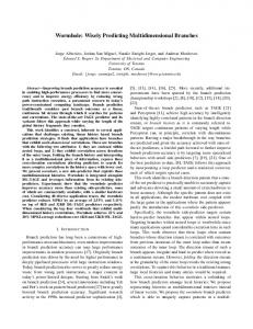
Figure 1. (a) Refactoring transformation rule R1 for adding getters and setters. (b) Initial partial model M1 of our motivating example. (c) Resulting partial model M2 after applying R1 to M1 .

achieve this by lifting, i.e., adapting, the semantics of ordinary transformations to partial models. We now present a motivating example. The partial modeling approach can be applied to any modeling language, but in this example we use a simplified version of UML class diagrams. We assume the scenario where a modeler is facing uncertainty regarding a fragment of the class diagram for an application for a food company. At the start of our scenario, the modeler has come up with the partial model M1 , shown in Figure 1(b) (see Section II for details about notation and semantics). M1 captures a basic hierarchy: a class Milk that extends a more general class Product. The modeler does not yet know if the company plans to use the application for non-perishables as well. She is therefore unclear as to whether expirationDate should be an attribute of all products or just for milk.1 At the same time, she is yet undecided as to whether an attribute hasExpired, derived from expirationDate, would be useful. The four possible alternative designs (also called concretizations), m1,1 − m1,4 , that this partial model encodes are shown in Figures 2(a-d). We further assume that the modeler wants to refactor the model to add getter and setter methods. For that she wants to 1 We

disregard the obvious modeling solution for illustration purposes.

We conclude our motivating example by introducing a second example transformation. After applying R1 to M1 and producing M2 , the modeler realizes that applying this rule had the undesired effect of also adding setter methods for the derived attribute hasExpired. For illustration purposes, we assume that derived attributes follow the naming convention “hasX”. Based on this, the modeler defined the transformation R2 , shown in Figure 3(a) (in the remainder of the paper, we refer to it as An Example Deleting Rule). The rule matches classes that have both a derived attribute and its respective setter and deletes this setter. Applying R2 to M2 should result in a new partial model M3 , shown in Figure 3(b), that has exactly the four concretizations m3,1 − m3,4 , shown in Figures 2(c-f). To summarize, the paper makes the following contributions: (a) We define the notion of lifting transformations to partial models and outline a way to test it. (b) We provide a method for defining semantics of lifting transformations for partial models using logical encodings in the form of transfer predicates. (c) We demonstrate the approach by applying it to two transformation examples and discuss the limitations and challenges of lifting (Section V).

Figure 2. (a-d) The four concretizations of M1 . (e-h) Concretizations of M2 , i.e., transformed versions of (a-d) respectively after the addition of getters and setters.

use a simple rewrite rule R1 (in the remainder of the paper, we refer to it as An Example Adding Rule) which is shown in Figure 1(a). The left-hand side (LHS) of the rule can match an attribute of a class. The matched sub-model is then replaced with the right-hand side (RHS) of the rule, which contains the newly added getter and setter operations. Applying a rule to a single classical model is straightforward, both in terms of desired results and of mechanics. But what does it mean to apply a transformation rule to a partial model? We break down this general question into two specific ones: (Q1) What should the result of applying a transformation to a partial model be? (Q2) What is the mechanics of applying a rule to a partial model? Regarding (Q1), we describe the intuition as follows: the partial model M1 in Figure 1(b) encodes exactly the four models m1,1 − m1,4 in Figure 2(a-d). Applying the rule R1 , using the “standard” graph transformation approach [3] to each alternative classical model m1,i in produces a new model m2,i , respectively shown in Figures 2(e-h).2 Models m2,1 − m2,4 are encoded by the partial model M2 shown in Figure 1(c). Therefore, the application of the rule R1 directly to M1 should result in M2 . We formalize this intuition as a correctness criterion in Section IV. Regarding (Q2), we have opted to not change the transformation itself, but rather redefine the semantics of rule application for partial models, using logic. In Section II, we describe how both classical and partial models can be encoded in propositional logic. In Section III-A, we outline a method to also encode the rules as transfer predicates and in Section III-B, we describe how to apply such encoded rules on partial models.

II. PARTIAL M ODELS In this section, we use the motivating example from Section I to briefly explain the notation and semantics of partial models. Their formal definition, semantics, encodings and representation are described in detail in [6]. The partial model M1 in Figure 1(b), called a May Model [11], summarizes the four alternative concretizations in Figure 2(a-d) compactly and exactly. Each element in M1 is annotated as True, False or Maybe [8]. A Maybe annotation indicates an optional element, such as the attributes labeled with the letters A to D in Figure 1(b). These are the model elements that differ between the concretizations and are depicted graphically using dashed lines. As more information becomes available, the annotations of these elements can change from Maybe to True or False (i.e., be included or excluded from the model) or remain Maybe. This process is a form of “point-wise” refinement [11] that only affects the degree of explicated uncertainty without introducing additional elements. A concretization of a partial model is a model where all the Maybe elements have been annotated with True or False. All concretizations of a partial model are classical and are obtained via point-wise refinement. We denote the set of concretizations of a partial model M by [M ]. May models are accompanied by May Formulas constraining the allowable configurations of the Maybe elements and thus defining the set of concretizations of the partial model. For example, the May formula for model M1 is Φmay = M1 (A ↔ ¬C) ∧ (B → A) ∧ (D → C). A particular valuation of Φmay M1 , namely, hA = True, B = C = D = Falsei, corresponds to the classical model m1,2 , shown in Figure 2(b). Every classical model is a partial model where all terms are annotated by True or False and the May formula is True.

2 We assume a graph transformation engine that applies the rule in parallel to all matching sites. For example, in the model m1,3 in Figure 2(c), the rule matches simultaneously both attributes, resulting in the model m2,3 in Figure 2(g).

2

all matched sites with RHS, to produce the output model N . That is, a rule R can be applied to an input model M to R∗ produce a new model N . We denote this as M =⇒ N . While inspired from algebraic graph transformation [3], we adopt a purely logic-based perspective of model transformation. A transformation is accordingly captured as a transfer predicate that relates elements of the input and the output models. In this section, we outline our approach for encoding and applying transformation rules as transfer predicates. A. Representing Transformations A transformation rule can be encoded in logic: Definition 3: Given a rule R = hLHS,RHSi, where ΦL , ΦR are propositional formula patterns, that logically encode the rule’s LHS and RHS respectively, the transfer predicate R(R) encodes the relationship between the variables of ΦL and those of ΦR as follows: R(R) = (ΦL → ΦR ) ∧ (¬ΦL → ΦN E ), where ΦN E describes the case where the rule has “no effect”. Matching is done by unifying the variables of ΦL , ΦR with those of the model at each particular site. That is, the rule says that if the LHS applies, then in the result (denoted by primed variables), RHS should hold. Otherwise, values of variables are left unchanged. Systematic construction of transfer predicates is still work in progress. In the following, we outline the manual construction of transfer predicates for the two rules of the motivating scenario.

Figure 3. (a) Refactoring transformation rule R2 for removing setters of derived attributes. (b) The partial model M3 resulting from applying R2 to M2 . (c-f) Concretizations of M3 .

A partial model (and thus every classical model as well!) can be encoded entirely as a propositional formula [6]. This is done by conjoining its May Formula with a conjunction of the model’s True and False elements. For the model M1 , this propositional encoding is the conjunction ΦM1 = Product ∧ Milk ∧ gen Milk Product ∧ . . .∧Φmay M1 , where gen Milk Product represents the generalization between Milk and Product.3 Moreover, the propositional formula for a partial model can be obtained by computing a disjunction of encodings for each of its concretizations. The set of all variables in such a propositional encoding is called the scope or vocabulary of the partial model. It is possible to embed a partial model into a larger scope, i.e., one that contains elements not present in the original. The new elements simply appear negated in the propositional encoding. For example, M1 can be embedded into the scope of M2 , in which case its propositional encoding becomes ΦM1 ∧ ¬E ∧ . . . ∧ ¬L.

An Example Adding Rule. The rule R1 , shown in Figure 1(a), is a refactoring rule that adds getters and setters for attributes in classes that don’t have them. Overall, the rule has four propositional variables: a class c, an attribute a, a getter g and a setter s. The rule’s LHS explicitly refers to the first two variables, c and a whereas the variables g, s are implicitly set to False (i.e., the rule does not match sites where the getter and the setter already exist). The rule’s RHS sets the variables of g 0 , s0 depending on the value of a. A matched site is captured by ΦL = c ∧ a ∧ ¬g ∧ ¬s. It is evident that at each matched site, the transfer predicate includes the expression Φ0R = (c0 ↔ c) ∧ (a0 ↔ a) ∧ (g 0 ↔ a) ∧ (s0 ↔ a)5 . For each model element x that is not matched by the rule, the transfer predicate is ΦN E = (x0 ↔ x).

III. PARTIAL T RANSFORMATIONS In the motivating scenario presented in Section I, the modeler uses graphical rules to express transformations. Traditionally, rules and their applications are defined as follows: Definition 1: A transformation rule R is a tuple hLHS, RHSi, where the typed, attributed graphs LHS, RHS are respectively called the left-hand and right-hand sides of the rule.4 Definition 2: A rule R = hLHS, RHSi is applied to a model M by finding all matches of LHS in M and replacing

An Example Deleting Rule. The rule R2 , shown in Figure 3(a), deletes the setters for derived attributes, assuming that the naming convention “hasX” is followed. This rule has three propositional variables: a class c, a derived attribute h and a setter s. The RHS of the rule implicitly sets s0 to False. A matched site is captured by ΦL = c ∧ h ∧ s. At each matched site, the transfer predicate is Φ0R = (c0 ↔ c)∧(h0 ↔ h) ∧ ¬s0 . For each model element x that is not matched by the rule, the transfer predicate is again ΦN E = (x0 ↔ x).

3 We have omitted the ownership relationships between attributes and classes for brevity. 4 We simplify the problem by ignoring negative application conditions [3]

5 The

3

operator ↔ is interpreted as equality.

B. Applying Transformations R(R1 , M1 , M2 )

When using the logical representations of models and transfer predicates, rule application is defined as: Definition 4: A rule R = hLHS, RHSi, applied to a (partial) model M to produce the output model N , corresponds to the equation Φ0N = R(R, M, N ) ∧ ΦM , where R(R, M, N ) is a transfer predicate, expressed in first-order logic, that associates the (primed) elements of N with the (unprimed) elements of M . The transfer predicate R(R, M, N ) is constructed by unifying the predicate R(R) with each site in M and N . Multiple applications of rules can be achieved by the construction: Φn = Φn−1 ∧ R(Rn , M n−1 , M n ). In this paper, we assume for simplicity that the vocabulary of the output model is known at the time of rule application. With this assumption, the Transfer Predicate is propositionalized over the union of the vocabularies of M and N .

Using the propositional encoding ΦM1 of the partial model R1 ∗ M1 , the production M1 =⇒ M2 is thus encoded as ΦM2 = R(R1 , M1 , M2 ) ∧ ΦM1 Example Deleting Rule (Cont’d). We now demonstrate the application of rule R2 to M2 . Using the vocabulary of M2 and manually doing the match for hc, h, si, we get two matching sites {hProduct, B, Hi, hMilk, D, Li}. The transfer predicate becomes R(R2 , M2 , M3 )

Rule Application for Classical Models: Example. We illustrate Definition 4 by creating the transfer predicate for applying the rule R1 to the model m1,1 in Figure 2(a). The construction is done manually by doing the matching and grounding over the union of the vocabularies of m1,1 and the model m2,1 in Figure 2(e). The rule matches the variables hc, a, g, si at the matching site hMilk, C, I, Ji. Thus, after simplification, the grounded transfer predicate becomes R(R1 , m1,1 , m2,1 )

= (Product0 ↔ Product) ∧ (Milk0 ↔ Milk)∧ (A0 ↔ A) ∧ (B 0 ↔ B) ∧ (C 0 ↔ C)∧ (D0 ↔ D) ∧ (E 0 ↔ A) ∧ (F 0 ↔ A)∧ (G0 ↔ B) ∧ (H 0 ↔ B) ∧ (I 0 ↔ C)∧ (J 0 ↔ C) ∧ (K 0 ↔ D) ∧ (L0 ↔ D)∧ (gen Milk Product0 ↔ gen Milk Product)

= (Product0 ↔ Product) ∧ (Milk0 ↔ Milk)∧ (B 0 ↔ B) ∧ (D0 ↔ D) ∧ ¬H 0 ∧ ¬L0 ∧ ΦN E

Here we used ΦN E to denote a conjunction of terms of the form (X 0 ↔ X) for each model element that was not matched by the rule, such as expirationDate, R2 ∗ getHasExpired, etc. The production M2 =⇒ M3 is encoded as ΦM3 = R(R2 , M2 , M3 ) ∧ ΦM2 using the propositional encoding ΦM2 of the partial model M2 . In this section, we showed how to encode an outcome of applying a transformation to models, partial and classical. This gives as semantics of partial transformations and answers question Q2 posted in Section I. Our treatment was based on knowing what the outcome of the transformation is supposed to be, since the output model was an integral part of computing the transfer predicate. In the next section, we discuss what such output model should be (question Q1).

= (Milk0 ↔ Milk) ∧ (C 0 ↔ C) ∧ (I 0 ↔ C)∧ (J 0 ↔ C) ∧ (Product0 ↔ Product)∧ (gen Milk Product0 ↔ gen Milk Product)

The last two clauses of the conjunction are the elements in the model that are unaffected by the transformation. Given the propositional encoding Φm1,1 of the model m1,1 , the R ∗

1 production m1,1 =⇒ m2,1 is consequently encoded as

Φm2,1 = R(R1 , m1,1 , m2,1 ) ∧ Φm1,1

IV. T OWARDS V ERIFICATION OF C ORRECTNESS This mechanism for applying transformations is directly applicable to the transformation of partial models. The only difference is that partial models have somewhat more complex encoding as propositional formulas. We illustrate on two examples below.

In this section, we define a criterion that lifted transformations should follow and check correctness of adding and deleting rules in our running example. Correctness Condition. Partial models are intended to be exact representations of sets of models and lifted transformations must preserve this. This means that applying a lifted transformation R to a partial model M should be equivalent to applying its classical version to each of the concretizations of M and building a partial model from the result. We refer to this principle as the Correctness Criterion for lifting transformations. More formally: Definition 5: Given a rule R, a partial model M with a set of concretizations [M ] = {m1 , . . . , mn }, and the set U = R∗ R∗ {m0i |∀mi ∈ [M ] · mi =⇒ m0i }, the production M =⇒ N is correct iff the set of concretizations of the resulting partial model M 0 satisfies the condition [N ] = U .

Example Adding Rule (Cont’d). We begin by encoding R1 ∗ the production M1 =⇒ M2 . Using the union of the vocabularies of the models M1 , M2 , shown in Figures 1(bc), we manually perform the matching and propositionalize the transfer predicate at the possible matching sites in M1 . For the variables hc, a, g, si, these are four matches: {hProduct, A, E, F i, hProduct, B, G, Hi, hMilk, C, I, Ji, hMilk, D, K, Li}. The only element unaffected by the rule in this case is the generalization gen Milk Product). After simplifying and removing duplicates, the transfer predicate becomes: 4

ning the SAT solver in ALLSAT mode. Comparing the valuations produced by MathSAT4 for each formula, we verified that the two formulas have the same sets of possible valuations, thus satisfying the correctness criterion. R2 ∗ Similarly, we tested the production M2 =⇒ M3 . We compared the valuations of the formulas ΦM3 = R(R2 , M2 , M3 ) ∧ ΦM2 and ΦU 3 . The latter was constructed similarly to ΦU 2 above for the models {m3,1 , m3,2 , m3,3 , m3,4 }, shown in Figures 3(c-f). Using MathSAT4, we verified that the sets of valuations of these formulas coincide, thus satisfying the correctness criterion. For these small examples, the runtimes of the SAT solver were negligible. As discussed in Section V, we do expect scalability issues for transformations of partial models with larger sets of concretizations and/or more sites of application. The overall process is expensive, due to the fact that in order to do a test, we have to enumerate and transform each concretization of the input model.

R∗

Figure 4. Testing the rule application M =⇒ N for correctness of lifting: (a) model view; (b) logical view.

Alternatively, the resulting model N is obtained by building a partial model from the set U . Note that this correctness criterion holds independently of how we choose to encode productions! Testing Correctness. Using this criterion, we can test R∗ whether a production M =⇒ N is correct with respect to lifting. Testing is done in three steps: (1) create the model N by applying the rule, (2) create the set U by appling the rule to each concretization m of M , (3) compare the sets [N ] and U . The process is summarized in Figure 4(a). The reason why we call this testing rather than verification is that we can only establish that the production is correct w.r.t. an input model M. In our motivating example, correctness of our encoding R1 ∗ of the production M1 =⇒ M2 can be tested by checking whether the set of concretizations [M2 ] is the same as the set of models that is constructed by individually transforming the set of concretizations [M1 ]. Indeed, by individually transforming the set {m1,1 , m1,2 , m1,3 , m1,4 } of concretizations of M1 , shown in Figures 2(a-d), we arrive to the set of models {m2,1 , m2,2 , m2,3 , m2,4 }, shown in Figures 2(e-h), which is exactly the set [M2 ].

V. S UMMARY AND D ISCUSSION Transforming partial models is an important component of the research agenda for partial models that we presented in [5], which aims to build a comprehensive framework for explicitly handling uncertainty in the software engineering lifecycle. In Section I, we presented the problem of transforming partial models in terms of two basic questions: (Q1) what should the outcome look like, and (Q2) what mechanics would produce such an outcome. We have outlined our preliminary thoughts on this: In Section IV, we defined a correctness criterion to answer (Q1). In Section III, we presented our approach to addressing (Q2), using a logicbased approach for defining the semantics of transformations that takes into account partial models. We further experimented with two examples of transformations, an additive and a deleting transformation. In this section, we draw from this experience to outline the major challenges that we have identified and discuss future steps. In Section IV, we used the correctness criterion to test the lifting of our example transformations, using SAT. Certain important limitations arose from these examples:

Towards Tool Support. Our encoding of transformations using the transfer predicate allows us to automatically check correctness of transformations using a SAT solver. R∗ In particular, given a production M =⇒ N , we compare the sets of valuations of the following two formulas: (a) the rule application formula ΦN = R(R, M, N ) ∧ ΦM and (b) the formula ΦU = Φm01 ∨ . . . ∨ Φm0k . ΦU encodes the set U of individually transformed concretizations. Each such concretization m0i is encoded by the formula Φm0i = R(R, mi , m0i ) ∧ Φmi . The process is summarized in Figure 4(b). We illustrate this verification approach using our example. R1 ∗ In order to check the correctness of the production M1 =⇒ M2 , we first construct the formula ΦM2 = R(R1 , M1 , M2 ) ∧ ΦM1 , as discussed in Section III-B. Subsequently, we create the formula ΦU 2 which represents the set of transformed concretizations {m2,1 , m2,2 , m2,3 , m2,4 }, that are shown in Figures 2(e-h). We used these formulas as inputs to MathSAT4 [1], run-

R ∗

1 1) Testing the production, e.g. M1 =⇒ M2 requires the U construction of the formula Φ2 that encodes the individually transformed concretizations of M1 . Essentially, this amounts to the explicit construction and enumeration of all the concretizations of M2 . This corresponds to thorough checking [7] and can be very expensive, especially if the set of concretizations of M1 is large or if there are many possible matching sites. 2) The criterion can only be used to test the application of a lifted transformation for specific input and output models. We should be able to verify that a transformation is correctly lifted, regardless of specific inputs and outputs. We are currently working on alternative approaches to verifying lifted transformations compositionally. For this, we aim to use an approach centered on proving transformations correct, based on identifying proof obligations, similar to the

5

(AHLR) [4]. We have made some initial attempts at formalizing partial models as an AHLR, with the biggest challenge being the identification of the proper morphisms. In conclusion, in this paper we have outlined the problem of partial model transformation and identified its main parameters in terms of correctness and mechanics. We have illustrated our preliminary approach in two examples of basic additive and deleting transformations. Using this experience we were able to identify the main challenges and outline next steps. R EFERENCES

approach we developed in [10] for verifying the special class of uncertainty-reducing partial model refinements. A logic-based lifting semantics for partial model transformation was introduced in Section III and illustrated on our two examples. Our preliminary attempts point us to identify the following challenges: 1) We manually constructed the transfer predicates for the particular examples we presented. Similarly, rule application was also done manually (matching and propositionalization of the transfer predicates). We are currently working on systematizing the creation of transfer predicates using First-Order Logic. Given a classical transformation, we want to create the transfer predicate using a predefined set of reusable modular predicates, such as MatchNode() AddNode(), DeleteEdge(), etc. This will allow us to support more sophisticated features of model transformation, such as Negative Application Conditions. At the same time, this will help streamline the lifting process and form the basis for effective tool support for automatic matching and propositionalization. 2) In our examples, we required knowledge of the vocabulary of the output model prior to rule application, especially in the case of additive transformations. This is, naturally, not always the case in real-world settings. A similar problem occurs with deleting transformations: deleted elements remain in the vocabulary, albeit negated. We are working on a more systematic approach to expand and contract vocabularies and, more specifically, on ways to treat transformations that affect changes to the vocabulary. 3) Applying transformations using the transfer predicate results in a formula that is in terms of the original model in the form of “unprimed variables”. Converting this to a representation that is useful to the user requires us to construct an expression that is solely expressed in terms of the resulting model. To do this, unprimed variables need to be factored out, which can be expensive. An alternative approach, that would address the last concern, but also provide a more general solution, would be to define partial model transformations in terms of the Double Pushout (DPO) approach [2]. In [3], it is proven that the DPO can be applied to any Adhesive High-Level Replacement Category

[1] R. Bruttomesso, A. Cimatti, A. Franzen, A. Griggio, and R. Sebastiani. The MathSAT 4 SMT Solver. In Proceedings of CAV’08’, pages 299–303, 2008. [2] A. Corradini, U. Montanari, F. Rossi, H. Ehrig, R. Heckel, and M. Lowe. Algebraic approaches to graph transformation. Part I: Basic concepts and double pushout approach. In Handbook of graph grammars and computing by graph transformation, pages 163–245. World Scientific Publishing Co., Inc., 1997. [3] H. Ehrig, K. Ehrig, U. Prange, and G. Taentzer. Fundamentals of Algebraic Graph Transformation. EATCS. Springer, 2006. [4] H. Ehrig, A. Habel, J. Padberg, and U. Prange. Adhesive High-Level Replacement Categories and Systems. Graph Transformations, 3256:144–160, 2004. [5] M. Famelis, S. Ben-David, M. Chechik, and R. Salay. “Partial Models: A Position Paper”. In Proceedings of MoDeVVa’11, pages 1–6, 2011. [6] M. Famelis, M. Chechik, and R. Salay. “Partial Models: Towards Modeling and Reasoning with Uncertainty”. In Proceedings of ICSE’12, 2012. To appear. [7] A. Gurfinkel and M. Chechik. “How Thorough Is Thorough Enough?”. In Proceedings of CHARME’05, pages 65–80, 2005. [8] K. G. Larsen and B. Thomsen. “A Modal Process Logic”. In Proceedings of LICS’88, pages 203–210, 1988. [9] M. Petre. “Insights from Expert Software Design Practice”. In Proceedings of FSE’09, 2009. [10] R. Salay, M. Chechik, and J. Gorzny. “Towards a Methodology for Verifying Partial Model Refinements”, 2012. submitted. [11] R. Salay, M. Famelis, and M. Chechik. “Language Independent Refinement using Partial Modeling”. In Proceedings of FASE’12, 2012.

6