The spin-foam-representation of loop quantum gravity

arXiv:gr-qc/0601095v1 23 Jan 2006

Edited by

1 The spin-foam-representation of LQG Alejandro Perez Centre de Physique Théorique, Campus de Luminy, 13288 Marseille, France. Unité Mixte de Recherche (UMR 6207) du CNRS et des Universités Aix-Marseille I, Aix-Marseille II, et du Sud Toulon-Var; laboratoire afilié ` a la FRUMAM (FR 2291).

Abstract

The problem of background independent quantum gravity is the problem of defining a quantum field theory of matter and gravity in the absence of an underlying background geometry. Loop quantum gravity (LQG) is a promising proposal for addressing this difficult task. Despite the steady progress of the field, dynamics remains to a large extend an open issue in LQG. Here we present the main ideas behind a series of proposals for addressing the issue of dynamics. We refer to these constructions as the spin foam representation of LQG. This set of ideas can be viewed as a systematic attempt at the construction of the path integral representation of LQG. The spin foam representation is mathematically precise in 2+1 dimensions, so we will start this chapter by showing how it arises in the canonical quantization of this simple theory. This toy model will be used to precisely describe the true geometric meaning of the histories that are summed over in the path integral of generally covariant theories. In four dimensions similar structures appear. We call these constructions spin foam models as their definition is incomplete in the sence that at least one of the following issues remains unclear: 1) the connection to a canonical formulation, and 2) regularization independence (renormalizability). In the second part of this chapter we will describe the definition of these models emphasizing the importance of these open issues. 1

2

Alejandro Perez 1.1 The path integral for generally covariant systems

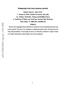
LQG is based on the canonical (Hamiltonian) quantization of general relativity whose gauge symmetry is diffeomorphism invariance. In the Hamiltonian formulation the presence of gauge symmetries (Dirac P.M.) gives rise to relationships among the phase space variables—schematically C(p, q) = 0 for (p, q) ∈ Γ—which are referred to as constraints. The constraints restrict the set of possible states of the theory by requiring them to lay on the constraint hyper-surface. In addition, through the Poisson bracket, the constraints generate motion associated to gauge transformations on the constraint surface (see Fig. (1.1)). The set of physical states (the so called reduced phase space Γred ) is isomorphic to the space of orbits, i.e., two points on the same gauge orbit represent the same state in Γred described in different gauges (Fig. 1.1). In general relativity the absence of a preferred notion of time implies that the Hamiltonian of gravity is a linear combination of constraints. This means that Hamilton equations cannot be interpreted as time evolution and rather correspond to motion along gauge orbits of general relativity. In generally covariant systems conventional time evolution is pure gauge: from an initial data satisfying the constraints one recovers a spacetime by selecting a particular one-parameter family of gauge-transformations (in the standard ADM context this amounts for choosing a particular lapse function N (t) and shift N a (t)). Γ quantizing

Γred

quantizing

Hkin

reducing

reducing

rbi eo ug ga

CONSTRAINT SURFACE

(spin foam rep)

Γ t

Constraint Hamiltonian vector field

Hphys

Γred

Fig. 1.1. On the left: the geometry of phase space in gauge theories. On the right: the quantization path of LQG (continuous arrows).

From this perspective the notion of spacetime becomes secondary and the dynamical interpretation of the the theory seems problematic (in the quantum theory this is refered to as the “problem of time”). A

The spin-foam-representation of LQG

3

possible reason for this apparent problem is the central role played by the spacetime representation of classical gravity solutions. However, the reason for this is to a large part due to the applicability of the concept of test observers (or more generally test fields) in classical general relativity†. Due to the fact that this idealization is a good approximation to the (classical) process of observation the notion of spacetime is useful in classical gravity. As emphasized by Einstein with his hole argument (see Rovelli C. (2005) for a modern explanation) only the information in relational statements (independent of any spacetime representation) have physical meaning. In classical gravity it remains useful to have a spacetime representation when dealing with idealized test observers. For instance to solve the geodesic equation and then ask diff-invariant-questions such as: what is the proper time elapsed on particle 1 between two succesive crossings with particle 2? However, already in the classical theory the advantage of the spacetime picture becomes, by far, less clear if the test particles are replaced by real objects coupling to the gravitational field †. However, this possibility is no longer available in quantum gravity where at the Planck scale (ℓp ≈ 10−33 cm) the quantum fluctuations of the gravitational field become so important that there is no way (not even in principle‡) to make observations without affecting the gravitational field. In this context there cannot be any, a priori, notion of time and hence no notion of spacetime is possible at the fundamental level. A spacetime picture would only arise in the semi-classical regime with the identification of some subsystems that approximate the notion of test observers. What is the meaning of the path integral in the background independent context? The previous discussion rules out the conventional † Most (if not all) of the textbook applications of general relativity make use of this concept together with the knowledge of certain exact solutions. In special situations there are even preferred coordinate systems based on this notion which greatly simplify interpretation (e.g. co-moving observers in cosmology, or observers at infinity for isolated systems). † In this case one would need first to solve the constraints of general relativity in order to find the initial data representing the self-gravitating objects. Then one would have essentially two choices: 1) Fix a lapse N (t) and a shift N a (t), evolve with the constraints, obtain a spacetime (out of the data) in a particular gauge, and finally ask the diff-invariant-question; or 2) try to answer the question by simply studying the data itself (without t-evolution). It is far from obvious whether the first option (the conventional one) is any easier than the second. ‡ In order to make a Planck scale observation we need a Planck energy probe (think of a Planck energy photon). It would be absurd to suppose that one can disregard the interaction of such photon with the gravitational field treating it as test photon.

4

Alejandro Perez

interpretation of the path integral. There is no meaningful notion of transition amplitude between states at different times t1 > t0 or equivalently a notion of “unitary time evolution” represented by an operator U (t1 − t0 ). Nevertheless, a path integral representation of generally covariant systems arises as a tool for implementing the constraints in the quantum theory as we argue below. Due to the difficulty associated with the explicit description of the reduced phase space Γred , in LQG one follows Dirac’s prescription. One starts by quantizing unconstrained phase space Γ, representing the canonical variables as self-adjoint operators in a kinematical Hilbert space Hkin . Poisson brackets are replaced by commutators in the standard way, and the constraints are promoted to self-adjoint operators (see Fig. 1.1). If there are no anomalies the Poisson algebra of classical constraints is represented by the commutator algebra of the associated quantum constraints. In this way the quantum constraints become the infinitesimal generators of gauge transformations in Hkin . The physical Hilbert space Hphys is defined as the kernel of the constraints, and hence associated to gauge invariant states. Assuming for simplicity that there is only one constraint we have ψ ∈ Hphys

iff

ˆ exp[iN C]|ψi = |ψi ∀ N ∈ R,

ˆ is the unitary operator associated to the gauge where U (N ) = exp[iN C] transformation generated by the constraint C with parameter N . One can characterize the set of gauge invariant states, and hence construct Hphys , by appropriately defining a notion of ‘averaging’ along the orbits generated by the constraints in Hkin . For instance if one can make sense of the projector Z P : Hkin → Hphys where P := dN U (N ). (1.8) It is apparent from the definition that for any ψ ∈ Hkin then P ψ ∈ Hphys . The path integral representation arises in the representation of the unitary operator U (N ) as a sum over gauge-histories in a way which is technically analogous to standard path integral in quantum mechanics. The physical interpretation is however quite different as we will show in Sec. 1.2.4. The spin foam representation arises naturally as the path integral representation of the field theoretical analog of P in the context of LQG. Needles is to say that many mathematical subtleties appear when one applies the above formal construction to concrete examples (Giulini D. & Marolf D., (1999)).


5

1.2 Spin foams in 3d quantum gravity Here we derive the spin foam representation of LQG in a simple solvable example: 2+1 gravity. For the definition of spin foam models directly in the covariant picture see Freidel (2005), and other approaches to 3d quantum gravity see Carlip S. (1998).

1.2.1 The classical theory Riemannian gravity in 3 dimensions is a theory with no local degrees of freedom, i.e., a topological theory. Its action (in the first order formalism) is given by Z S[e, ω] = Tr(e ∧ F (ω)), (1.9) M

where M = Σ × R (for Σ an arbitrary Riemann surface), ω is an SU (2)connection and the triad e is an su(2)-valued 1-form. The gauge symmetries of the action are the local SU (2) gauge transformations δe = [e, α] ,

δω = dω α,

(1.10)

where α is a su(2)-valued 0-form, and the ‘topological’ gauge transformation δe = dω η,

δω = 0,

(1.11)

where dω denotes the covariant exterior derivative and η is a su(2)-valued 0-form. The first invariance is manifest from the form of the action, while the second is a consequence of the Bianchi identity, dω F (ω) = 0. The gauge symmetries are so large that all the solutions to the equations of motion are locally pure gauge. The theory has only global or topological degrees of freedom. Upon the standard 2+1 decomposition, the phase space in these variables is parametrized by the pull back to Σ of ω and e. In local coordinates one can express them in terms of the 2-dimensional connection Aia and the triad field Ejb = ǫbc ekc δjk where a = 1, 2 are space coordinate indices and i, j = 1, 2, 3 are su(2) indices. The Poisson bracket is given by {Aia (x), Ejb (y)} = δab δ ij δ (2) (x, y).

(1.12)

Local symmetries of the theory are generated by the first class constraints Db Ejb = 0,

i Fab (A) = 0,

(1.13)

6

Alejandro Perez

which are referred to as the Gauss law and the curvature constraint respectively. This simple theory has been quantized in various ways in the literature, here we will use it to introduce the spin foam representation.

1.2.2 Spin foams from the Hamiltonian formulation The physical Hilbert space, Hphys , is defined by those ‘states in Hkin ’ that are annihilated by the constraints. As discussed in Thiemann (2005) (see also Rovelli C. (2005) and Thiemann (2005)), spin network states a \ solve the Gauss constraint—D a Ei |si = 0—as they are manifestly SU (2) gauge invariant. To complete the quantization one needs to characterize i the space of solutions of the quantum curvature constraints Fbab , and to provide it with the physical inner product. As discussed in Sec. 1.1 we can achieve this if we can make sense of the following formal expression for the generalized projection operator P : Z Z Y P = D[N ] exp(i Tr[N Fb (A)]) = δ[F[ (A)], (1.14) Σ

x⊂Σ

where N (x) ∈ su(2). Notice that this is just the field theoretical analog of equation (1.8). P will be defined below by its action on a dense subset of test-states called the cylindrical functions Cyl ⊂ Hkin (see Ashtekar & Lewandowski (2004)). If P exists then we have hsP U [N ], s′ i = hsP, s′ i ∀ s, s′ ∈ Cyl, N (x) ∈ su(2) (1.15) R where U [N ] = exp(i Tr[N Fˆ (A)]). P can be viewed as a map P : Cyl → KF ⊂ Cyl⋆ (the space of linear functionals of Cyl) where KF denotes the kernel of the curvature constraint. The physical inner product is defined as hs′ , sip := hs′ P, si,

(1.16)

where h, i is the inner product in Hkin , and the physical Hilbert space as Hphys := Cyl/J

for J := {s ∈ Cyl s.t. hs, sip = 0},

(1.17)

where the bar denotes the standard Cauchy completion of the quotient space in the physical norm. One can make (1.14) a rigorous definition if one introduces a regularization. A regularization is necessary to avoid the naive UV divergences that appear in QFT when one quantizes non-linear expressions of the

7


canonical fields such as F (A) in this case (or those representing interactions in standard particle physics). A rigorous quantization is achieved if the regulator can be removed without the appearance of infinities, and if the number of ambiguities appearing in this process is under control (more about this in Sec. 1.3.1). We shall see that all this can be done in the simple toy example of this section.

Wp ε

Σ

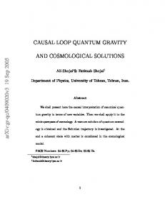
Fig. 1.2. Cellular decomposition of the space manifold Σ (a square lattice of size ǫ in this example), and the infinitesimal plaquette holonomy Wp [A].

We now introduce the regularization. Given a partition of Σ in terms of 2-dimensional plaquettes of coordinate area ǫ2 (Fig. 1.2) one can write the integral Z X F [N ] := Tr[N F (A)] = lim ǫ2 Tr[Np Fp ] (1.18) ǫ→0

Σ

p

as a limit of a Riemann sum, where Np and Fp are values of the smeari ing field N and the curvature ǫab Fab [A] at some interior point of the ab plaquette p and ǫ is the Levi-Civita tensor. Similarly the holonomy Wp [A] around the boundary of the plaquette p (see Figure 1.2) is given by Wp [A] = 1 + ǫ2 Fp (A) + O(ǫ2 ).

(1.19) P

The previous two equations imply that F [N ] = limǫ→0 p Tr[Np Wp ], and lead to the following definition: given s, s′ ∈ Cyl (think of spin network states) the physical inner product (1.16) is given by Y Z hs′ P, si := lim hs dNp exp(iTr[Np Wp ]), si. (1.20) ǫ→0

p

The partition is chosen so that the links of the underlying spin network graphs border the plaquettes. One can easily perform the integration over the Np using the identity (Peter-Weyl theorem) Z X j (2j + 1) Tr[Π (W )], (1.21) dN exp(iTr[N W ]) = j

8

Alejandro Perez j

where Π (W ) is the spin j unitary irreducible representation of SU (2). Using the previous equation np (ǫ)

hs′ P, si := lim

ǫ→0

Y X jp (2jp + 1) hs′ Tr[Π (Wp )]), si, p

(1.22)

jp

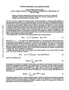
where the spin jp is associated to the p-th plaquette, and np (ǫ) is the number of plaquettes. Since the elements of the set of Wilson loop operators {Wp } commute, the ordering of plaquette-operators in the previous product does not matter. The limit ǫ → 0 exists and one can give a closed expression for the physical inner product. That the regulator can be removed follows from the orthonormality of SU (2) irreducible representations which implies that the two spin sums associated to the action of two neighboring plaquettes collapses into a single sum over the action of the fusion of the corresponding plaquettes (see Fig 1.3). One can also show that it is finite†, and satisfies all the properties of an inner product (Noui K. & Perez A. (2005)).

P

=

(2j + 1)(2k + 1) j

jk

k

P

(2k + 1)

k

k

Fig. 1.3. In two dimensions the action of two neighboring plaquette-sums on the vacuum is equivalent to the action of a single larger plaquette action obtained from the fusion of the original ones. This implies the trivial scaling of the physical inner product under refinement of the regulator and the existence of a well defined limit ǫ → 0.

1.2.3 The spin foam representation jp

Each Tr[Π (Wp )] in (1.22) acts in Hkin by creating a closed loop in the jp representation at the boundary of the corresponding plaquette (Figs. 1.4 and 1.6). Now, in order to obtain the spin foam representation we introduce a non-physical (coordinate time) as follows: Instead of working † The physical inner product between spin network states satisfies the following inequality X hs, s′ ip ≤ C (2j + 1)2−2g , j

for some positive constant C. The convergence of the sum for genus g ≥ 2 follows

9


k

Tr[Π (Wp )] ⊲

P

j

=

P

k

Nj,m,k

j

m

m

.

Fig. 1.4. Graphical notation representing the action of one plaquette holonomy on a spin network state. On the right is the result written in terms of the spin network basis. The amplitude Nj,m,k can be expressed in terms of ClebschGordan coefficients.

with one copy of the space manifold Σ we consider np (ǫ) copies as a jp

n (ǫ)

p . Next we represent each of the Tr[Π (Wp )] discrete folliation {Σp }p=1 in (1.22) on the corresponding Σp . If one inserts the resolution of unity in Hkin between the slices, graphically

1=

X

|γ, {j}ihγ, {j}|

γ⊂Σ,{j}γ

Σ2 Σ1

coordinate time

Σ3

(1.23)

where the sum is over the complete basis of spin network states {|γ, {j}i}— based on all graphs γ ⊂ Σ and with all possible spin labelling—one arrives at a sum over spin-network histories representation of hs, s′ ip . More precisely, hs′ , sip can be expressed as a sum over amplitudes corresponding to a series of transitions that can be viewed as the ‘time evolution’ between the ‘initial’ spin network s′ and the ‘final’ spin network s. This is illustrated in the two simple examples of Figs. 1.5 and 1.7); on the r.h.s. we illustrate the continuum spin foam picture obtained when the regulator is removed in the limit ǫ → 0. Spin network nodes evolve into edges while spin network links evolve into 2-dimensional faces. Edges inherit the intertwiners associated to the nodes and faces inherit the spins associated to links. Therefore, the directly. The case of the sphere g = 0 and the torus g = 1 can be treated individually (Noui K. & Perez A. (2005)).

10

Alejandro Perez j

j

j

k

k

m

k

k

k

k

m

m

m

m

j

k

j

j

j

m

m j

j j

j

k

m

k

k

k

m

m

m

m

j

Fig. 1.5. A set of discrete transitions in the loop-to-loop physical inner product obtained by a series of transitions as in Figure 1.4. On the right, the continuous spin foam representation in the limit ǫ → 0. j

k

j P

n

Tr[Π (Wp )] ⊲

=

P

o,p

m

1 ∆n ∆j ∆k ∆m

j k m n o p

k

n

p

o m

.

.

Fig. 1.6. Graphical notation representing the action of one plaquette holonomy on a spin network vertex. The object in brackets ({}) is a 6j-symbol and ∆j := 2j + 1.

series of transitions can be represented by a 2-complex whose 1-cells are labelled by intertwiners and whose 2-cells are labelled by spins. The places where the action of the plaquette loop operators create new links (Figs. 1.6 and 1.7) define 0-cells or vertices. These foam-like structures are the so-called spin foams. The spin foam amplitudes are purely combinatorial and can be explicitly computed from the simple action of the loop operator in Hkin . The physical inner product takes the standard Ponzano-Regge form when the spin network states s and s′ have only 3-valent nodes. Explicitly, j5

j4

hs, s′ ip =

X

Y

Fs→s′ f ⊂Fs→s′

(2jf + 1)

νf 2

Y

v⊂Fs→s′

j3 j6 j1

,

(1.24)

j2

where the sum is over all the spin foams interpolating between s and s′ (denoted Fs→s′ , see Fig. 1.10), f ⊂ Fs→s′ denotes the faces of the spin

11


foam (labeled by the spins jf ), v ⊂ Fs→s′ denotes vertices, and νf = 0 if f ∩ s 6= 0 ∧ f ∩ s′ 6= 0, νf = 1 if f ∩ s 6= 0 ∨ f ∩ s′ 6= 0, and νf = 2 if f ∩ s = 0 ∧ f ∩ s′ = 0. The tetrahedral diagram denotes a 6j-symbol: the amplitude obtained by means of the natural contraction of the four intertwiners corresponding to the 1-cells converging at a vertex. More generally, for arbitrary spin networks, the vertex amplitude corresponds to 3nj-symbols, and hs, s′ ip takes the same general form. j

j

m

m

p

j

m

n

p

j

n o

o

k

k

k

j

j

j

p

p m

n

p m

n

o

o

n o

k

k

j

j

p

k

j

p

m

m

n

p m

n

o

k

o

m m

n

p

n

o

o

k

k

k

Fig. 1.7. A set of discrete transitions representing one of the contributing histories at a fixed value of the regulator. On the right, the continuous spin foam representation when the regulator is removed.

Even though the ordering of the plaquette actions does not affect the amplitudes, the spin foam representation of the terms in the sum (1.24) is highly dependent on that ordering. This is represented in Fig 1.8 where a spin foam equivalent to that of Fig 1.5 is obtained by choosing an ordering of plaquettes where those of the central region act first. One can see this freedom of representation as an analogy of the gauge freedom in the spacetime representation in the classical theory. j j

j

j

j

k

j

k

m

k

m

m

k

m

j k

m

j k

m

k

k j m

j k

m

j k

m

k m

j

Fig. 1.8. A different representation of the transition of figure 1.5. This spinfoam is obtained by a different ordering choice in (1.22).

12

Alejandro Perez

One can in fact explicitly construct a basis of Hphys by choosing an linearly independent set of representatives of the equivalence classes defined in (1.17). One of these basis is illustrated in Fig. 1.9. The number of quantum numbers necessary to label the basis element is 6g − 6 corresponding to the dimension of the moduli space of SU (2) flat connections on a Riemann surface of genus g. This is the number of degrees of freedom of the classical theory. In this way we arrive at a fully combinatorial definition of the standard Hphys by reducing the infinite degrees of freedom of the kinematical phase space to finitely many by the action of the generalized projection operator P . 3

6g−10

6g−6

6g−8 6g−7

6g−9

6g−11

6g−13 6g−14

1 4

5

2

6g−12

Fig. 1.9. A spin-network basis of physical states for an arbitrary genus g Riemann surface. There are 6g − 6 spins labels (recall that 4-valent nodes carry an intertwiner quantum number).

1.2.4 Quantum spacetime as gauge-histories What is the geometric meaning of the spin foam configurations? Can we identify the spin foams with “quantum spacetime configurations”? The answer to the above questions is, strictly speaking, in the negative in agreement with our discussion at the end of Sec. 1.1. This conclusion can be best illustrated by looking first at the simple example in 2+1 gravity where M = S 2 × R (g = 0). In this case the spin foam configurations appearing in the transition amplitudes look locally the same to those appearing in the representation of P for any other topology. However, a close look at the physical inner product defined by P permits to conclude that the physical Hilbert space is one dimensional—the classical theory has zero degree of freedom and so there is no non-trivial Dirac observable in the quantum theory. This means that the sum over spin foams in (1.24) is nothing else but a sum over pure gauge degrees of freedom and hence no physical interpretation can be associated to it. The spins la-


13

belling the intermediate spin foams do not correspond to any measurable quantity. For any other topology this still holds true, the true degrees of freedom being of a global topological character. This means that in general (even when local excitations are present as in 4d) the spacetime geometric interpretation of the spin foam configurations is subtle. This is an important point that is often overlooked in the literature: one cannot interpret the spin foam sum of (1.24) as a sum over geometries in any obvious way. Its true meaning instead comes from the averaging over the gauge orbits generated by the quantum constraints that defines P —recall the classical picture Fig. 1.1, the discussion around eq. (1.8), and the concrete implementation in 2+1 where U (N ) in (1.15) is the unitary transformation representing the orbits generated by F . Spin foams represent a gauge history of a kinematical state. A sum over gauge histories is what defines P as a means for extracting the true degrees of freedom from those which are encoded in the kinematical boundary states. l

p o

q

j

n k

s

m n

p q

s

m

l j k

l

o

j k l j k

Fig. 1.10. A spin foam as the ‘colored’ 2-complex representing the transition between three different spin network states. A transition vertex is magnified on the right.

Here we studied interpretation of the spin foam representation in the precise context of our toy example; however, the validity of the conclusion is of general character and holds true in the case of physical interest four dimensional LQG. Although, the quantum numbers labelling the spin foam configurations correspond to eigenvalues of kinematical geometric quantities such as length (in 2+1) or area (in 3+1) LQG, their physical meaning and measurability depend on dynamical considerations (for instance the naive interpretation of the spins in 2+1 gravity as quanta of physical length is shown here to be of no physical relevance). Quantitative notions such as time, or distance as well as qualitative statements about causal structure or time ordering are misleading (at

14

Alejandro Perez

best) if they are naively constructed in terms of notions arising from an interpretation of spin foams as quantum spacetime configurations†.

1.3 Spin foam models in four dimensions We have studied 2+1 gravity in order to introduce the qualitative features of the spin foam representation in a precise setting. Now we discuss some of the ideas that are pursued for the physical case of 3+1 LQG. Spin foam representation of canonical LQG There is no complete construction of the physical inner product of LQG in four dimensions. The spin foam representation as a device for its definition was originally introduced in the canonical formulation by Rovelli (see Rovelli C. (2005)). In 4-dimensional LQG difficulties in understanding dynamics are centered around understanding the space of solutions ˆ The physical inner product formally of the quantum scalar constraint S. becomes  n Z Z ∞ n X i  ′ b  s, s′ idiff , (1.25) h N (x)S(x) hP s, s idiff = D[N ] n! n=0 Σ

where h , idiff denotes the inner product in the Hilbert space of diffinvariant states, and the exponential in (the field theoretical analog of) (1.8) has been expanded in powers. Smooth loop states are naturally annihilated by Sb (independently of any quantization ambiguity (Jacobson T. & Smolin L. (1988) and Smolin L. & Rovelli, C. (1990))). Consequently, Sb acts only on spin network nodes. Generically, it does so by creating new links and nodes modifying the underlying graph of the spin network states (Figure 1.11). k

j

R

Σ

b N (x)S(x) ⊲

= m

j

P

n

k

n

o

p

p

o

N (xn )Snop m

nop

k j m

.

.

Fig. 1.11. The action of the scalar constraint and its spin foam representation. b N (xn ) is the value of N at the node and Snop are the matrix elements of S.

In a way that is qualitatively similar to what we found in the concrete

† The discussion of this section is a direct consequence of Dirac’s perspective applied to the spin foam representation.

15


implementation of the curvature constraint in 2+1 gravity, each term in the sum (1.25) represents a series of transitions—given by the local action of Sb at spin network nodes—through different spin network states interpolating the boundary states s and s′ respectively. The action of Sˆ can be visualized as an ‘interaction vertex’ in the ‘time’ evolution of the node (Figure 1.11). As in 2+1 dimensions, equation (1.25) can be pictured as sum over ‘histories’ of spin networks pictured as a system of branching surfaces described by a 2-complex whose elements inherit the representation labels on the intermediate states (see Fig. 1.10). The value of the ‘transition’ amplitudes is controlled by the matrix elements b of S. Spin foam representation in the Master Constraint Program

The previous discussion is formal. One runs into technical difficulties if one tries to implement the construction of the 2+1 gravity in this case. The main reason for this is the fact that the constrain algebra does not close with structure constants in the case of 3+1 gravity†. In order to circumvent this problem Thiemann recently proposed to impose one single master constraint defined as Z S 2 (x) − q ab Va (x)Vb (x) p , (1.26) M = dx3 det q(x) Σ

where q ab is the space metric and Va (x) is the vector constraint. Using techniques developed by Thiemann this constraint can indeed be promoted to a quantum operator acting on Hkin . The physical inner product could then be defined as ′

hs, s ip := lim hs, T →∞

ZT

c

dt eitM s′ i.

−T

(1.27)

A spin-foam-representation of the previous expression is obtained by splitting the t-parameter in discrete steps and writing c c c/n]n . eitM = lim [eitM /n ]n = lim [1 + itM n→∞

n→∞

(1.28)

† In 2+1 gravity the constraint algebra correspond to the Lie algebra of ISO(3) (isometries of Euclidean flat spacetime). There are no local degrees of freedom and the underlying gauge symmetry has a non dynamical structure. In 3+1 gravity the presence of gravitons changes that. The fact that the constraint algebra closes with structure functions means that the gauge symmetry structure is dynamical or field dependent. This is the key difficulty in translating the simple results of 2+1 into 3+1 dimensions.

16

Alejandro Perez

The spin foam representation follows from the fact that the action of the c/n on a spin network can be written as a linear basic operator 1 + itM combination of new spin networks whose graphs and labels have been modified by the creation of new nodes (in a way qualitatively analogous to the local action shown in Figure 1.11). An explicit derivation of the physical inner product of 4d LQG along these lines is under current investigation. Spin foam representation: the covariant perspective In four dimensions the spin foam representation of LQG has also been motivated by lattice discretizations of the path integral of gravity in the covariant formulation (for recent reviews see Perez A. (2003) and Oriti D. (2001)). In four dimensions there are two main lines of approach; both are based on classical formulations of gravity based on modifications of the BF-theory action. The first approach is best represented by the Barrett-Crane model (Barrett J.W. & Crane L. (1998)) and corresponds to the quantization attempt of the classical formulation of gravity based on the Plebanski action Z S[B, A, λ] = Tr [B ∧ F (A) + λ B ∧ B] , (1.29) where B is an so(3, 1)-valued two-form λ is a Lagrange multiplier imposing a quadratic constraint on the B’s whose solutions include the sector B = ⋆(e ∧ e), for a tetrad e, corresponding to gravity in the tetrad formulation. The key idea in the definition of the model is that the path integral for BF-theory, whose action is S[B, A, 0], Z Z Ptopo = D[B]D[A] exp i Tr [B ∧ F ] (1.30) can be defined in terms of spin foams by a simple generalization of the construction of Sec. 1.2. Notice that the formal structure of the action S[B, A, 0] is analogous to that of the action of 2+1 gravity (1.9) (see Baez J.C. (2000)). The Barrett-Crane model aims at providing a definition of the path integral of gravity formally written as Z Z PGR = D[B]D[A] δ [B → ⋆(e ∧ e)] exp i Tr [B ∧ F ] , (1.31) where the measure D[B]D[A]δ[B → ⋆(e∧e)] restricts the sum in (1.30) to those configurations of the topological theory satisfying the constraints B = ⋆(e∧e) for some tetrad e. The remarkable fact is that the constraint


17

B = ⋆(e ∧ e) can be directly implemented on the spin foam configurations of Ptopo by appropriate restriction on the allowed spin labels and intertwiners. All this is possible if a regularization is provided, consisting of a cellular decomposition of the spacetime manifold. The key open issue is however how to get rid of this regulator. A proposal for a regulator independent definition is that of the group field theory formulation (Oriti D. (2005)). A second proposal is the one recently introduced by Freidel and Starodubtsev 2005 based on the formulation McDowell-Mansouri action of Riemannian gravity given by Z α (1.32) S[B, A] = Tr[B ∧ F (A) − B ∧ Bγ5 ], 4 where B is an so(5)-valued two-form, A an so(5) connection, α = GΛ/3 ≈ 10−120 a coupling constant, and the γ5 in the last term produces the symmetry braking SO(5) → SO(4). The idea is to define PGR as a power series in α, namely Z Z ∞ X (−iα)n n PGR = D[B]D[A](Tr[B ∧ Bγ ]) exp i Tr[B ∧ F ] . 5 4n n! n=0 Notice that each term in the sum is the expectation value of a certain power of B’s in the well understood topological BF field theory. A regulator in the form of a cellular decomposition of the spacetime manifold is necessary to give a meaning to the former expression. Due to the absence of local degrees of freedom of BF-theory it is expected that the regulator can be removed in analogy to the 2+1 gravity case. It is important to show that removing the regulator does not produce an uncontrollable set of ambiguities (see remarks below regarding renormalizability).

1.3.1 The UV problem in the background independent context In the spin foam representation, the functional integral for gravity is replaced by a sum over amplitudes of combinatorial objects given by foam-like configurations (spin foams). This is a direct consequence of the background independent treatment of the gravitational field degrees of freedom. As a result there is no place for the UV divergences that plague standard quantum field theory. The combinatorial nature of the fundamental degrees of freedom of geometry appears as a regulator of all the interactions. This seem to be a common feature of all the formulations referred to in this chapter. Does it mean that the UV problem in LQG

18

Alejandro Perez

is resolved? The answer to this question remains open for the following reason. All the definitions of spin foams models require the introduction of some kind of regulator generically represented by a space (e.g., in the canonical formulation of 2+1 gravity or in the master-constraint program) or spacetime lattice (e.g. in the Barrett-Crane model or in the Freidel-Starodubtsev prescription). This lattice plays a role of a UV regulator in more or less the same sense as a UV cut-off (Λ) in standard QFT. The UV problem in standard QFT is often associated to divergences in the amplitudes when the limit Λ → ∞ is taken. The standard renormalization procedure consists of taking that limit while appropriately tuning the bare parameters of the theory so that UV divergences cancel to give a finite answer. Associated to this process there is an intrinsic ambiguity as to what values certain amplitudes should take. These must be fixed by appropriate comparison with experiments (renormalization conditions). If only a finite number or renormalization conditions are required the theory is said to be renormalizable. The ambiguity of the process of removing the regulator is an intrinsic feature of QFT. The background independent treatment of gravity in LQG or the spin foam models we have described here do not escape to this general considerations (Perez A. (2005)). Therefore, even though no UV divergences can arise as a consequence of the combinatorial structure of the gravitational field, the heart of the UV problem is now to be found in the potential ambiguities associated with the elimination of the regulator. This remains an open problem for all the attempts of quantization of gravity in 3+1 dimensions. The problem takes the following form in each of the approaches presented in this chapter: • The removal of the regulator in the 2+1 case is free of ambiguities and hence free of any UV problem (Perez A. (2005)). • In the case of the master constraint program one can explicitly show that there is a large degree of ambiguity associated to the regularization procedure (Perez A. (2005)). It remains to be shown whether this ambiguity is reduced or disappears when the regulators are removed in the definition of P . • The Barrett-Crane model is discretization dependent. No clear-cut prescription for the elimination of the triangulation dependence is known. • The Freidel-Starodubtsev prescription suffers (in principle) from the ambiguities associated to the definition of the expectation value of the


19

B-monomials appearing in (1.33) before the regulator is removed†. It is hoped that the close relationship with a topological theory might cure these ambiguities although this remains to be shown. Progress in the resolution of this issue in any of these approaches would represent a major breakthrough in LQG.

Acknowledgements I would like to thank M. Mondragon and A. Mustatea for careful reading of the manuscript and D. Oriti for his effort and support in this project.

References Dirac P.M. (). Lectures on Quantum Mechanics Rovelli C. (2005). Quantum Gravity. Cambridge: Cambridge Univ. Press. Giulini D. & Marolf D., (1999). On the generality of refined algebraic quantization. Class. Quant. Grav., 16, 2479. Thiemann T. (2005). . Cambridge: Cambridge Univ. Press. Ashtekar A. & Lewandowski J. (2004). Background independent quantum gravity: A status report. Class. Quant. Grav., 21 R53. Thiemann, T. (2005) in Towards Quantum Gravity, Cambridge: Cambridge Univ. Press. (to appear) Carlip S. (1998). Quantum gravity in 2+1 dimensions. Cambridge: Cambridge Univ. Press. Noui K. & Perez A. (2005). Three dimensional loop quantum gravity: Physical scalar product and spin foam models. Class. Quant. Grav, 22, 4489–4514. Perez A. (2003). Spin foam models for quantum gravity. Class. Quant. Grav, 20, R43. Oriti D. (2001). Spacetime geometry from algebra: Spin foam models for nonperturbative quantum gravity. Rept. Prog. Phys., 64, 1489–1544. Jacobson T. & Smolin L. (1988). Nonperturbative quantum geometries. Nucl. Phys., B299, 295. Smolin L. & Rovelli, C. (1990). Loop space representation of quantum general relativity. Nucl. Phys., B331, 80. Barrett J.W. & Crane L. (1998). Relativistic spin networks and quantum gravity. J.Math.Phys., 39, 3296-3302. Baez J.C. (2000). An Introduction to Spin Foam Models of Quantum Gravity and BF Theory. Lect.Notes Phys., 543, 25–94. Freidel L. & Starodubtsev A. (2005). Quantum gravity in terms of topological observables. arXiv:hep-th/0501191. † There are various prescriptions in the literature on how to define this monomials. They are basically constructed in terms of the insertion of appropriate sources to construct a BF generating function. All of them are intrinsically ambiguous, and the degree of ambiguity grows with the order of the monomial. The main source of ambiguity resides in the issue of where in the discrete lattice to act with the functional source derivatives.

20

Alejandro Perez

Oriti D. (2005) in Towards Quantum Gravity, Cambridge: Cambridge Univ. Press. (to appear) Perez A. (2005). On the regularization ambiguities in loop quantum gravity. arXiv:gr-qc/0509118.