The Stochastic complexity of spin models: Are pairwise models really

The Stochastic complexity of spin models: Are pairwise models really simple? Alberto Beretta,1 Claudia Battistin,2 Clélia de Mulatier,1 Iacopo Mastromatteo,3 and Matteo Marsili1

arXiv:1702.07549v3 [cond-mat.dis-nn] 11 Apr 2018

1

The Abdus Salam International Centre for Theoretical Physics (ICTP), Strada Costiera 11, I-34014 Trieste, Italy 2 Kavli Institute for Systems Neuroscience and Centre for Neural Computation, NTNU, Olav Kyrres gate 9, 7030 Trondheim, Norway 3 Capital Fund Management, 23 rue de l’Université, 75007 Paris, France Models can be simple for different reasons: because they yield a simple and computationally efficient interpretation of a generic dataset (e.g. in terms of pairwise dependences) – as in statistical learning – or because they capture the essential ingredients of a specific phenomenon – as e.g. in physics – leading to non-trivial falsifiable predictions. In information theory and Bayesian inference, the simplicity of a model is precisely quantified in the stochastic complexity, which measures the number of bits needed to encode its parameters. In order to understand how simple models look like, we study the stochastic complexity of spin models with interactions of arbitrary order. We highlight the existence of invariances with respect to bijections within the space of operators, which allow us to partition the space of all models into equivalence classes, in which models share the same complexity. We thus found that the complexity (or simplicity) of a model is not determined by the order of the interactions, but rather by their mutual arrangements. Models where statistical dependencies are localized on non-overlapping groups of few variables (and that afford predictions on independencies that are easy to falsify) are simple. On the contrary, fully connected pairwise models, which are often used in statistical learning, appear to be highly complex, because of their extended set of interactions. Keywords: Information theory | Statistical inference | Model complexity | Spin model

Science, as the endeavour of reducing complex phenomena to simple principles and models, has been instrumental to solve practical problems. Yet, problems such as image or speech recognition and language translation have shown that Big Data can solve problems without necessarily understanding [1–3]. A statistical model trained on a sufficiently large number of instances can learn how to mimic the performance of the human brain on these tasks [4, 5]. These models are simple in the sense that they are easy to evaluate, train and/or to infer. They offer simple interpretations in terms of low order (typically pairwise) dependencies, which in turn afford an explicit graph theoretical representation [6]. Their aim is not to uncover fundamental laws but to “generalize well”, i.e. to describe well yet unseen data. For this reason, machine learning relies on “universal” models that are apt to describe any possible data on which they can be trained [7], using suitable “regularization” schemes in order to tame parameter fluctuations (overfitting) and achieve small generalization error [8]. Scientific models, instead, are the simplest possible descriptions of experimental results. A physical model is a representation of a real system and its structure reflects the laws and symmetries of Nature. It predicts well not because it generalizes well, but rather because it captures essential features of the specific phenomena that it describes. It should depend on few parameters and is designed to provide predictions that are easy to be falsified [9]. For example, Newton’s laws of motion are consistent with momentum conservation, a fact that can be checked in scattering experiments. The intuitive notion of a “simple model” hints at a succinct description, one that requires few bits [10]. The

stochastic complexity [11], derived within Minimum Description Length (MDL) [12, 13], provides a quantitative measure for “counting” the complexity of models in bits. The question this paper addresses is: what are the features of simple models according to MDL and are they simple in the sense surmised in statistical learning or in physics? In particular, are models with up to pairwise interactions, which are frequently used in statistical learning, simple? We address this issue in the context of spin models, describing the statistical dependence among n binary variables. There has been a surge of recent interest in the inference of spin models [14] from high dimensional data, most of which was limited to pairwise models. This is partly because pairwise models allow for an intuitive graph representation of statistical dependencies. Most importantly, since the number of k-variable interactions grows as nk , the number of samples is hardly sufficient to go beyond k = 2. For this reason, efforts to go beyond pairwise interactions have mostly focused on low order interactions (e.g. k = 3, see [15] and references therein). Ref. [16] recently suggested that even for data generated by models with higher order interactions, pairwise models may provide a sufficiently accurate description of the data. Within the class of pairwise models, L1 regularization [17] has proven to be a remarkably efficient heuristic of model selection (but see also [18]). Here we focus on the exponential family of spin models with interactions of arbitrary order. This class of models assume a sharp separation between relevant observables and irrelevant ones, whose expected value is predicted by the model. In this setting, the stochastic complexity [11] computed within MDL coincides with the penalty that,

2 in Bayesian model selection, accounts for model’s complexity, under non-informative (Jeffrey’s) priors [19]. A.

The exponential family of spin models (with interactions of arbitrary order)

Consider n spin variables s = (s1 , . . . , sn ), taking values si = ±1. The probability distribution of s under a model M belonging to the exponential family is given by: P (s | g, M) with

= ZM1(g) e P P

ZM (g) =

s

e

P

µ∈M

µ∈M

µ

g µ φµ (s)

µ

g φ (s)

,

, (1) (2)

µ

where the model M is identified by the set Q {φ (s), µ ∈ M} of product spin operators, φµ (s) = i∈µ si . Each operator φµ (s) models the interaction that involves all the spins of the subset µ of the n spins. We thus consider interactions of any arbitrary order (see Appendix sec. SI0). For instance, for pairwise interaction models, the operators φµ (s) are single spins si or product of two spins si sj , for i, j ∈ {1, ..., n}. The g µ are the conjugate parameters1 that modulates the strength of the interaction associated with φµ . Finally, the partition function ZM (g) ensures normalisation. We remark that the models of (1) can be derived as the maximum entropy distributions that are consistent with the requirement that the model reproduces the empirical averages of the operators φµ (s) for all µ ∈ M on a given dataset [20, 21]. In other words, empirical averages of φµ (s) are sufficient statistics, i.e. their values are enough to compute the maximum likelihood parameters g ˆ. Therefore the choice of the operators φµ in M inherently entails a sharp separation between relevant variables (the sufficient statistics) and irrelevant ones, which may have important consequences in the inference process. For example, if statistical inference assumes pairwise interactions, it might be blind to relevant patterns in the data resulting from higher order interactions. Without prior knowledge, all models M should be compared. According to MDL and Bayesian model selection (see Appendix sec. SI-0), models should be compared on the basis of their maximum (log)likelihood corrected by their complexity. In other words, simple models should be preferred a priori. Stochastic complexity

The complexity of a model can be defined unambiguously within MDL as the number of bits needed to specify

1

There is a broader class of models, where subsets V ⊆ M of operators have the same parameter, i.e. g µ = g V for all µ ∈ V. These degenerate models are rarely considered in the inference literature. Here we confine our discussion to non-degenerate models and refer the reader to Appendix sec. SI-7 for more discussion.

a priori the parameters g ˆ that best describe a dataset sˆ = (s(1) , . . . , s(N ) ) consisting of N samples independently drawn from the distribution P (s | g, M) for some unknown g (see Appendix sec. SI-0). Asymptotically for N → ∞, for systems of discrete variables, the MDL complexity is given by [22, 23]: X |M| N log P (ˆ s|g ˆ, M) ' log + cM . (3) 2 2π s ˆ

The two terms in the r.h.s. are the stochastic complexity [11, 24]. The first term, which is the basis of the Bayesian Information Criterion (BIC) [24, 25], captures the increase of the complexity with the number |M| of model’s parameters and with the number N of data points. This accounts for the fact that the uncertainty in each parameter g ˆ decreases with N as N −1/2 , so its description requires ∼ 12 log N bits. The second term cM quantifies the statistical dependencies between the parameters, and it is given by Z p cM = log dg det J(g) , (4) where J(g) is the Fisher Information matrix with entries Jµν (g) =

∂2 log ZM (g). ∂g µ ∂g ν

(5)

The term cM encodes for the intrinsic notion of simplicity we are interested in. To distiguish these two terms, we will refer to the first as BIC term and to the second as stochastic complexity. For an exponential family, the MDL criteria (3) coincides with the Bayesian model selection approach, assuming Jeffreys’ prior over the parameters g [24, 26, 27] (see Appendix sec. SI-0). Within a fully Bayesian approach, the model that maximises its posterior given the data sˆ, P (M|ˆ s), is the one to be selected. Therefore, if two models have the same number of parameters (same BIC term), the simplest one, i.e. the one with the lowest stochastic complexity cM , has to be chosen a priori. However, the number of possible interactions φµ among n spins isn 2n − 1, and therefore the number of spin models is 22 −1 . The super-exponential growth of the number of models with the number of spins n makes selecting the simplest model unfeasible even for moderate n. Our aim is then to understand how the stochastic complexity depends on the structure of the model M and eventually provide guidelines for the search of simpler models in such a huge space. EQUIVALENCE CLASSES OF MODELS B.

Gauge transformations

Let’s start by showing that low order interactions do not have a privileged status and are not necessarily related to low complexity cM , with the following argument:

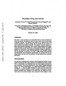
3 are not simplicial complexes. Model d) is invariant under any permutations of the four spins, whereas the other models have a lower degree of symmetry under permutations (see the different multiplicities in Fig. 1). Gauge transformations are discussed in more details in Appendix sec. SI-1. One can also see them as a change of the basis s → σ in which the operators are expressed. Counting the number of possible bases then gives us the number of gauge transformations (see Appendix sec. SI1): NGT (n) = 2n FIG. 1. Example of gauge transformations between models with n = 4 spins. Models are represented by diagrams (color online): spins are full dots • in presence of a local field, empty dots ◦ otherwise; blue lines are pairwise interactions (φµ = si sj ); orange triangles denote 3-spin interactions (φµ = si sj sk ); and the 4-spin interaction (s1 s2 s3 s4 ) is a filled blue triangle. Note that model a) has all its interactions grouped on 3 spins; the gauge transformations leading to this model are shown along the arrows. All the models belong to the same complexity class, with |M| = 7, λ = 4 and a number of independent operators nM = 3 (e.g. s1 , s2 and s3 in model a) – see tables in Appendix sec. SI-6). The class contains in total 15 models, which are grouped, with respect to the permutation of the spins, behind the 4 representatives shown here with their multiplicity (×m).

Alice is interested in finding which model M best describes a dataset sˆ; Bob is interested in the same problem, but his dataset σ ˆ is related to Alice’s dataset by a gauge transformation. The latter is defined as a bijective transformation between the n spin variables s of Alice and those of Bob, σ = (σ1 , · · · , σn ) ∈ {±1}n , that corresponds to a bijection from the set of all operators 0 to itself, φµ (s) → φµ (σ) (see the examples in Fig. 1 and Appendix sec. SI-1). This induces a bijective transformation between Alice’s models and those of Bob, as shown in Fig. 1, that preserves the number of interactions |M|. Whatever conclusion Bob draws on the relative likelihood of models can be translated into Alice’s world, where it has to coincide with Alice’s result. It follows that two models M and M0 related by a gauge transformation must also have the same complexity cM = cM0 . In particular, pairwise interactions can be mapped to interactions of any order (see Fig. 1), and, consequently, low order interactions are not necessarily simpler than higher order ones. Observe that models connected by gauge transformations have remarkably different structures. In Fig. 1, model a) has all the possible interactions concentrated on 3 spins, having the properties of a simplicial complex2 [28]; however, its gauge-transformed counterparties

2

A simplicial complex [28], in our notation, is a model such that,

2

n Y

k=1

1 − 2−k .

(6)

Notice that the number of gauge transformations, (6), is much smaller than the number 2n ! of possible bijections of the set of 2n states into itself. Indeed a generic bijection between the state spaces of s and σ maps each product operator to one of the binary functions f : σ → {+1, −1}, which does not necessarily correspond to a product operator φµ (σ). C.

Complexity classes

Gauge transformations allow us to divide the set of all models into equivalence classes, which we call complexity classes. Models belonging to the same class are related to each other by a gauge transformation (that is the equivalence relation), and thus have the same complexity cM . This classification suggests the presence of “quantum numbers” (invariants), in terms of which models can be classified. These invariants emerge explicitly when writing the cluster expansion of the partition function [29–31] (see Appendix sec. SI-2): Y X Y n µ ZM (g) = 2 cosh(g ) tanh(g µ ) . (7) µ∈M

`∈L µ∈`

The sum runs on the set L of all possible loops ` that can be formed with the operators µ ∈ M. A loop is any subQ set ` ⊆ M such that µ∈` φµ (s) = 1 for any value of s, i.e. such that each spin si occurs zero or an even number of times in this product. The set L includes the empty loop ` = ∅. The structure of ZM (g) in (7) depends on few characteristics of the model M: the number |M| of operators (or, equivalently, of parameters) and the structure of its set of loops L (which operator is involved in which loop). The invariance under gauge transformation of the complexity in (4) reveals itself in the fact that the partition function of models related by a gauge transformation have the same functional dependence on their parameters up to relabeling.

for any interaction µ ∈ M, any interaction that involves any subset ν ⊆ µ of spins is also contained in the model (i.e. ν ∈ M).

4 Let us focus on the loop structure of models belonging to the same class. The set L of loops of any model M has the structure of a finite Abelian group: if `1 , `2 ∈ L, then `1 ⊕`2 is also a loop of M, where ⊕ is the symmetric difference3 of two sets (see Appendix sec. SI-3). As a consequence, for each model M one can identify a minimal generating set of λ loops, such that any loop in L can be uniquely expressed as a product of loops in the minimal generating set. Note that the choice of the generating set is not unique, though all choices have the same cardinality λ; Fig. 2 gives examples of this decomposition for the models of Fig. 1. Note also that ` ⊕ ` = ∅ for each loop ` ∈ L. As a consequence, the cardinality of the loop group is |L| = 2λ (including the empty loop ∅). We found that λ is related to the number |M| of operators of the model by λ = |M| − nM (see Appendix sec. SI3), where nM is the number of independent operators of a model M, i.e. the maximal number of operators that can be taken in M without forming any loop. This implies that λ attains its minimal value, λ = 0, for models with only independent operators (|M| = nM ), and its maximal value, λ = 2n − 1 − n, for the complete model M, that contains all the |M| = 2n − 1 possible operators. The number of independent operators nM is preserved by gauge transformation, and, as the total number of operators |M| is also an invariant of the class, so is the cardinality of the minimal generating set λ. For example, all models in Fig. 1 have nM = 3 independent operators and λ = 4 (see Fig. 2). It can also be shown that gauge transformations imply a duality relation, that associates to each class of models with |M| operators a class of models with the 2n − 1 − |M| complementary operators (see Appendix sec. SI-3). Summarizing, the quantities |M| and nM , and the structure of L (through its generators) fully characterize a complexity class.

HOW DO SIMPLE MODELS LOOK LIKE? D.

Fewer independent operators, shorter loops

Coming to the quantitative estimate of the complexity, cM generally depends on the extent to which ensemble averages of the operators φµ (s) in the model µ ∈ M constrain each other. This appears explicitly by rewriting (4) as an integral over the ensemble averages of the operators, ϕ = {hφµ i, µ ∈ M}, exploiting the bijection between the parameters g and their dual parameters ϕ and re-parameterization invariance [27, 32]: Z p cM = log dϕ det J(ϕ) , (8) F

3

The symmetric difference of two sets `1 and `2 is the set that contains the elements that occur in `1 but not in `2 and viceversa: `1 ⊕ `2 = (`1 ∪ `2 ) \ (`1 ∩ `2 ). It corresponds to the XOR operator between the spins of the two loops.

a)

b)

c)

d)

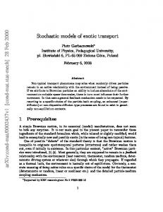
FIG. 2. Example of a minimal generating set of loops for each model of Fig. 1. As these models belong to the same class, their (respective) sets of loops have the same cardinality 2λ , where λ = 4 is the number of generators (as shown here). For model a), one can easily check that the 4 loops of the set are independent, as each of them contains at least one operator that doesn’t appear in the other 3 loops (see Appendix sec. SI3). Within each column, on the r.h.s., loops are related by the same gauge transformation morphing models into one another on the l.h.s. (i.e. the transformations displayed in Fig. 1). This shows that the loops of these 4 generating sets have the same structure, which implies that the loop structure of the 4 models is the same. Any loop of a model can finally be obtained by combining a subset of its generating loops. Note that the choice of the generating set is not unique.

where J(ϕ) is the Fisher Information Matrix in the ϕcoordinates. The new domain F of integration is over the values of ϕ that can be realized in any empirical sample drawn from the model M (known in this context as marginal polytope [33]) and is related to the mutual constraints between the ensemble averages ϕµ (see Appendix sec. SI-4 for more details). If the model contains no loop, i.e. L = {∅}, then Jµν (ϕ) = [1 − (ϕµ )2 ]−1 δµν is diagonal: the integral in (8) factorizes and gives cM = |M| log π. In this case, the variables ϕµ are not constrained at all and the domain of integration is F = [−1, 1]|M| . If instead the model contains loops, the variables ϕµ become constrained and the marginal polytope F is reduced. For example, for a model with a single loop of length three (e.g. φ1 = s1 , φ2 = s2 and φ3 = s1 s2 ), the values of ϕ in [−1, 1]3 are not all attainable, indeed F = {ϕ ∈ [−1, 1]3 : |ϕ1 + ϕ2 | − 1 ≤ ϕ3 ≤ 1 − |ϕ1 − ϕ2 |} is reduced, which decreases the complexity. The complexity cM (k) of models with a fixed number |M| of parameters and a single (non-empty) loop of length k is shown in Fig. 3 (see Appendix sec. SI-6): cM (k) increases with k and saturates at |M| log π, which is the value one would expect if all operators where unconstrained. This is consistent with the expectation that longer loops induce weaker constraints among the operators. Note that the number of independent operators is kept constant here, equal to nM = |M| − 1. The single loop calculation allows computing the complexity of models with non-overlapping loops (` ∩ `0 = ∅

5

FIG. 3. Complexity cM (k) of models with a single loop of length k, and |M| − k free operators, i.e. not involved in any loop. For k = 3, cM (3) = (|M| − 1) log π can be computed analytically from (4). Values of cM are averaged over 103 numerical estimates of the integral in (4), using 106 Monte Carlo samples each. Error bars correspond to their standard deviation.

P for all `, `0 ∈ L), for which cM = `∈L c` is the sum over the complexity c` associated to each loop. In the general case of models with more complex loop structures, the explicit calculation of cM is non-trivial. Yet, the argument above suggests that, at fixed number of parameters |M|, cM should increase with the number nM of independent operators. Fig. 4 summarises the results for all models with n = 4 spins and supports this conclusion: for a given value of |M|, classes with lower values of nM (i.e. with less independent operators) are less complex. A surprising result of Fig. 4 is that cM is not monotonic with the number |M| of operators of the model, increasing first with |M| and then decreasing. Complete models M turn out to be the simplest (see the dashed curve in Fig. 4). As a consequence, for a given |M|, models that contain a complete model on a subset of spins are generally simpler than models where operators have support on all the spins. For instance, the complexity class displayed in Fig. 1 is the class of models with |M| = 7 operators that has the lowest complexity (see green triangle on the dashed curve in Fig. 4). Fig. 4 also confirms that pairwise models are not simpler than models with higher order interactions. Indeed, for instance for |M| = 7, cM increases drastically when changing model a) of Fig. 1 into a pairwise model by turning the 3-spin interaction into an external field acting on s4 . Likewise, the model with all 6 pairwise interactions for |M| = 10 is more complex than the one where one of them is turned into a 3-spin interaction.

E.

FIG. 4. (color online) Complexity of models for n = 4 as a function of the number |M| of operators: each triangle represents a class of complexity, which contains one or more models (see Appendix sec. SI-6). For each class, the value of the cM was obtained from a representative of the class; some of them are shown here with their corresponding diagram (same notations as in Fig. 1). The triangle colors indicate the values of nM : violet for nM = 4, green for 3, yellow for 2, pink for 1 and red for 0 (model with no operator). Models on the black line have only independent operators (|M| = nM ) and complexity cM = |M| log π; models on the dashed curve are complete models, whose complexity is given in (9). Complexity classes with the same values of |M| and nM have the same value of λ = |M| − nM , i.e. the same number of loops |L|, but with a different structure.

strained by their normalization [34]. The complexity in (4) is invariant under reparametrization [32]. Re-writing this integralQin terms of the variables p(s) and using that det J(p) = s 1/p(s), we find (see Appendix sec. SI-5): ! Z 1 X Y 1 p , cM = log dp δ p(s) − 1 p(s) 0 s s = 2n−1 log π − log Γ(2n−1 ) .

(9)

Note that, for n > 4, cM becomes negative (for n = 6, cM ' −41.5). This suggests that the class of least complex models with |M| interactions is the one that contains the model where the maximal number of loops are concentrated on the smallest number of spins. This agrees with our previous observations on single loop models and sub-complete models. On the contrary, models where interactions are distributed uniformly across the variables (e.g. models with only single spin operators for n ≥ |M| or with non-overlapping sets of loops) have higher complexity.

Complete and sub-complete models F.

It is possible to compute explicitly the complexity of a complete model P M with n spins. Indeed, there is a mapping g µ = 2−n s φµ (s) log p(s) between the 2n − 1 parameters g µ of M and the 2n probability p(s), also con-

Maximally overlapping loops

This finally leads us to conjecture that stochastic complexity is related to the localization properties of the set of loops L (i.e. its group structure) rather

6 than to the order of the interactions: models where the loops `, `0 ∈ L have a “large” overlap ` ∩ `0 are simple, whereas models with an extended homogeneous network of interactions (e.g. fully connected Ising models with up-to pairwise interaction) have many non-overlapping loops ` ∩ `0 = ∅ and therefore are rather complex. It is interesting to note that the former (simple models) lend themselves to predictions on the independence of different groups of spins. These predictions suggest “fundamental” properties of the system under study (i.e. invariance properties, spin permutation symmetry breaking) and are easy to falsify (i.e. it is clear how to devise a statistical test for these hypotheses to any given confidence level). On the contrary, complex models (e.g. fully connected pairwise Ising models) are harder to falsify as their parameters can be adjusted to fit reasonably well any sample, irrespectively of the system under study.

G.

Summary

We find that at fixed number |M| of operators, simpler models are those with fewer independent operators (i.e. smaller nM ). For the same value of nM , models can still have different complexities. The simpler ones are then those with a loop structure that will impose the most constraints between the operators of the model. More generally, we show that the complexity of a model is not defined by the order of the interactions involved, but is, instead, intimately connected to its internal geometry, i.e. how interactions are arranged in the model. The geometry of this arrangement implies mutual dependencies between interactions, that constrain the states accessible to the system. More complex models are those that implement fewer constraints, and can thus account for broader types of data. This result is consistent with the information geometric approach of Ref. [24], which studies model complexity in terms of the geometry of the space of probability distributions4 . The contribution of this paper clarifies the relation between the information geometric point of view and the specific structure of the model, i.e. the actual arrangement of its interactions. A rough estimate of the number N of data samples beyond which the complexity term becomes negligible in Bayesian inference can be obtained with the following argument: An upper bound for the complexity of models with n spins and m parameters is given by m log π, i.e. when all operators are independent. As a lower bound, we take Eq. (9) with m = 2n − 1. This implies that an upper bound for the variation of the complexity is given

4

In information geometry [27, 32], a model M defines a manifold in the space of probability distributions. For exponential models (1), the natural metric, in the coordinates g µ , is given by the Fisher Information (5), and the stochastic complexity (4) is the volume of the manifold [24].

m+1 by ∆c = m−1 . When this is much 2 log π + log Γ 2 smaller than the BIC term, the stochastic complexity can be neglected. For large m this implies N m, which may be relevant for the applicability of fully connected pairwise models (m ' n2 /2) in typical cases, for instance when samples cannot be considered as independent observations from a stationary distribution (see [18]). CONCLUSION

As pointed out by Wigner [35] long ago, the unreasonable effectiveness of mathematical models relies on isolating phenomena that depend on few variables, whose mutual variation is described by simple models and is independent of the rest. Remarkably we find that, for a fixed number of spin variables and parameters, simple models, according to MDL, are precisely of this form: statistical dependencies are concentrated on the smallest subset of variables and these are independent of all the rest. Such simple models are not optimal to generalize, i.e. to describe generic statistical dependencies, rather they are easy to falsify. They are designed for spotting independencies that may hint at deeper principles (e.g. symmetries or conservation laws) that may “take us beyond the data” 5 . On the contrary, fully connected pairwise models appears to be rather complex. This, we conjecture, is the origin of pairwise sufficiency [16] that makes them so successful to describe a wide variety of data from neural tissues [36] to voting behaviour [37]. On the other hand, pairwise interactions play a special role in our understanding of phenomena as they allow to reduce statistical dependencies into direct interactions between variables. Therefore it would be important to identify methods to quantitatively assess when a dataset is genuinely described by pairwise interactions. The results of this paper allow one to address this issue by comparing inference with pairwise models to inference with models obtained via their gauge transformations. Since the latter preserve the number of interactions and the stochastic complexity, transformed models have the same flexibility in terms of generalisation. For the same reason, the comparison between pairwise models and their gauge transformed ones can be done on the basis of likelihood alone. In conclusion, our results suggest that when data are scarce and high dimensional, Bayesian inference should privilege simple models, i.e. those with small stochastic complexity, over more complex ones, such as fully connected pairwise models that are often used [14, 36, 37]. A full Bayesian model selection approach is hampered by the calculation of the stochastic complexity that is

5

In his response to Ref. [2] on edge.org, W.D. Willis observes that “Models are interesting precisely because they can take us beyond the data”.

7 a daunting task. Developing approximate heuristics for accomplishing this task is a challenging future avenue of research.

[1] V. Mayer-Schonberger and K. Cukier, Big Data: A Revolution That Will Transform How We Live, Work and Think. (John Murray Publishers, UK, 2013). [2] C. Anderson, Wired Magazine (2008). [3] N. Cristianini, Neural Networks 23, 466 (2010). [4] Y. LeCun, K. Kavukcuoglu, and C. Farabet, in Circuits and Systems (ISCAS), Proceedings of 2010 IEEE International Symposium on (IEEE, 2010) pp. 253–256. [5] A. Hannun, C. Case, J. Casper, B. Catanzaro, G. Diamos, E. Elsen, R. Prenge, S. Satheesh, S. Sengupta, A. Coates, and A. Ng, ArXiv e-prints (2014), arXiv:1412.5567 [cs.CL]. [6] C. Bishop, Pattern Recognition and Machine Learning, Information Science and Statistics (Springer, 2006). [7] X. Wu, V. Kumar, J. Ross Quinlan, J. Ghosh, Q. Yang, H. Motoda, G. J. McLachlan, A. Ng, B. Liu, P. S. Yu, Z.-H. Zhou, M. Steinbach, D. J. Hand, and D. Steinberg, Knowledge and Information Systems 14, 1 (2008). [8] I. Goodfellow, Y. Bengio, and A. Courville, Deep Learning (MIT Press, 2016) http://www.deeplearningbook. org. [9] K. Popper, The Logic of Scientific Discovery, Routledge Classics (Taylor & Francis, 2005). [10] N. Chater and P. Vit´ anyi, Trends in cognitive sciences 7, 19 (2003). [11] J. Rissanen, Journal of Computer and System Sciences 55, 89 (1997). [12] J. Rissanen, Automatica 14, 465 (1978). [13] P. D. Gr¨ unwald, The minimum description length principle (MIT press, 2007). [14] H. Chau Nguyen, R. Zecchina, and J. Berg, ArXiv eprints (2017), arXiv:1702.01522 [cond-mat.dis-nn]. [15] A. Margolin, K. Wang, A. Califano, and I. Nemenman, IET Syst Biol 4, 428 (2010). [16] L. Merchan and I. Nemenman, Journal of Statistical Physics 162, 1294 (2016). [17] P. Ravikumar, M. J. Wainwright, and J. D. Lafferty, The Annals of Statistics 38, 1287 (2010). [18] N. Bulso, M. Marsili, and Y. Roudi, Journal of Statistical Mechanics: Theory and Experiment 2016, 093404 (2016). [19] V. Balasubramanian, Neural computation 9, 349 (1997).

ACKNOWLEDGMENTS

C. B. acknowledges financial support from the Kavli Foundation and the Norwegian Research Council’s Centre of Excellence scheme (Centre for Neural Computation, grant number 223262). A. B. acknowledges financial support from International School for Advanced Studies (SISSA).

[20] E. T. Jaynes, Physical Review 106, 620 (1957). [21] Y. Tikochinsky, N. Z. Tishby, and R. D. Levine, Physical Review A 30, 2638 (1984). [22] J. J. Rissanen, IEEE Transactions on Information Theory 42, 40 (1996). [23] J. Rissanen, IEEE Transactions on Information Theory 47, 1712 (2001). [24] I. J. Myung, V. Balasubramanian, and M. A. Pitt, Proceedings of the National Academy of Sciences 97, 11170 (2000). [25] G. Schwarz, The annals of statistics 6, 461 (1978). [26] H. Jeffreys, Proceedings of the Royal Society of London A: Mathematical, Physical and Engineering Sciences 186, 453 (1946). [27] S. Amari, Information Geometry and Its Applications, Applied Mathematical Sciences (Springer Japan, 2016). [28] O. T. Courtney and G. Bianconi, Physical Review E 93, 062311 (2016). [29] L. Landau and E. Lifshitz, Statistical Physics, v. 5 (Elsevier Science, 2013). [30] H. A. Kramers and G. H. Wannier, Physical Review 60, 263 (1941). [31] A. Pelizzola, Journal of Physics A: Mathematical and General 38, R309 (2005). [32] S. Amari and H. Nagaoka, Methods of Information Geometry, Translations of mathematical monographs (American Mathematical Society, 2007). [33] M. J. Wainwright and M. I. Jordan, Foundations and R in Machine Learning 1, 1 (2008). Trends [34] I. Mastromatteo, ArXiv e-prints (2013), arXiv:1311.0190 [cond-mat.stat-mech]. [35] E. P. Wigner, Communications on pure and applied mathematics 13, 1 (1960). [36] E. Schneidman, M. Berry, R. II, and W. Bialek, Nature 440, 1007 (2006). [37] E. Lee, C. Broedersz, and W. Bialek, Journal of Statistical Physics 160, 275 (2015). [38] M. J. Wainwright and M. I. Jordan, in PROCEEDINGS OF THE ANNUAL ALLERTON CONFERENCE ON COMMUNICATION CONTROL AND COMPUTING, Vol. 41 (Citeseer, 2003) pp. 961–971.

Supporting Information Appendix for: ”The Stochastic complexity of spin models: Are pairwise models really simple?” Alberto Beretta,1 Claudia Battistin,2 Clélia de Mulatier,1 Iacopo Mastromatteo,3 and Matteo Marsili1

arXiv:1702.07549v3 [cond-mat.dis-nn] 11 Apr 2018

1

The Abdus Salam International Centre for Theoretical Physics (ICTP), Strada Costiera 11, I-34014 Trieste, Italy 2 Kavli Institute for Systems Neuroscience and Centre for Neural Computation, NTNU, Olav Kyrres gate 9, 7030 Trondheim, Norway 3 Capital Fund Management, 23 rue de l’Université, 75007 Paris, France

SI-0.

GENERAL FRAMEWORK – SPIN MODELS SI-0.1.

Spin operators

Let us consider the system of n spin variables, s = (s1 , · · · , sn ), that take random values si = ±1. In order to account for interactions of any order, we associate to any interaction involving a subset µ of spins a spin operator φµ (s) defined as the product of all the spins in µ: Y φµ (s) = si , (1) i∈µ

which takes value in {+1, −1}. By definition, the total number of these operators corresponds to the number of possible interactions in the n-spin system, i.e. to the number of possible subsets of {s1 , . . . , sn }, empty set excluded, which is 2n − 1. In the following we simplify the notation of the operator label µ by using an integer, µ ∈ {1, . . . , 2n − 1}, whose binary representation directly identifies the spins that belong to the set µ 1 . For instance, the operator φ1 (s) = s1 is associated with a field acting on s1 , and φ7 (s) = s1 s2 s3 with a three body interaction. These spin operators are the building blocks of the models. Note that, these operators verify: X φµ (s) = 0 , µ ∈ {1, . . . , 2n − 1} , (2) s∈S

n

where S = {−1, 1} , and the sum over s ∈ S denotes the sum over all possible configurations of the spins. SI-0.2.

Complete set of spin operators

We define the set Ωn = {φµ (s)}µ∈{0,...,2n −1} of all the spin operators built with n spins, including also the operator φ (s) = 1 (which is not associated with any interaction). By definition, the cardinality of Ωn is |Ωn | = 2n . The set Ωn is (called) orthogonal and complete as its operators verify respectively the relations [1]: 0

n

1 X µ hφ (s), φ (s)i = n φ (s) φν (s) = δµ,ν 2 µ

ν

and

s∈S

2 −1 1 X µ φ (s) φµ (s0 ) = δs,s0 . 2n µ=0

(3)

The first relation defines an inner product h·, ·i over the space of operators Ωn . The relation derives from the fact that the product of two operators of Ωn is also an operator of Ωn : φµ (s) φν (s) = φµ⊕ν (s) ,

(4)

where, in the binary representation of µ and ν, ⊕ is the XOR bitwise operation. Using the property (2) and observing that φµ (s)φµ (s) = φ0 (s) = 1 gives the first relation. The second relation is an immediate consequence of the fact that, for the set of monomials Ωn , one has n 2X −1

µ=0

1

φµ (s) φµ (s0 ) =

X

α1 =0,1

···

n X Y

(si s0i )αi ,

(5)

αn =0,1 i=1

The spin si belongs to µ if the ith digit (starting from the right) in the binary representation of µ is “1”. For example, φ5 (s) = s1 s3 , since the binary representation of 5 is 0 . . . 0101, with “1” only in the 1rst and 3rd positions along the binary string of length n.

2 which is always equal to zero, unless all si are equal to s0i . In this latter case the sum yields the 2n factor that allows to recover (3). The orthogonality and completeness properties (3) allow us to express 2 any function F (s) as a linear combination of operators [1] φµ (s), i.e. X 1 X µ f µ φµ (s), and f µ = hF (s), φµ (s)i = n F (s) = φ (s)F (s). (6) 2 µ∈Ωn

s∈S

Generating set of Ωn and independent operators

In the following, we will call generating set of Ωn a set of n spin operators that can fully generate Ωn , such as the set {s1 , . . . , sn }. We also define the notion of set of independent operators 3 as a set I verifying that the product of all the operators of any subset of I is always different from φ0 (s) = 1. Formally, any set of n independent operators of Ωn is a generating set of Ωn . By definition, a generating set of Ωn cannot include the identity operator 1. Mathematically, the set Ωn , associated with the multiplication operation (Ωn , ·), forms a finite Abelian group with identity element φ0 (s) = 1 generated by a minimal set of n generators of order 2 (Ωn = Z2 n ). SI-0.3.

Spin models

A model M is defined in terms of a subset M ⊆ Ωn \{φ0 } of operators 4 . These define a probability distribution of the vector s = (s1 , . . . , sn ) of spin variables: P X P µ µ µ µ 1 e µ∈M g φ (s) where ZM (g) = e µ∈M g φ (s) , (7) P (s | g, M) = ZM (g) s∈S

µ

where the vector g = {g , µ ∈ M} are the conjugate parameters: each parameter g µ is a real variable that modulates ¯ = Ωn \{φ0 } with the strength of the interaction associated with the operator φµ (s). We shall refer to the model M all operators as the complete model. Models can be degenerate (several operators are mapped to the same parameter) or not. Non-degenerate models

Non-degenerate models are those for which each operator φµ (s) is assigned a different parameter g µ . For instance, model a) in Fig. 1 of the main text involves |M| = 7 interactions, mapping the 7 operators M = {s1 , s2 , s3 , s1 s2 , s1 s3 , s2 s3 , s1 s2 s3 } onto the 7 parameters g = {g 1 , g 2 , g 4 , g 3 , g 5 , g 6 , g 7 } (using the binary representation1 of µ). The number of different non-degenerate models with n spins grows superexponentially in n: n

Nn = 2|Ωn \{1}| = 22

−1

.

(8)

To give an idea: N2 = 8, N3 = 128, N4 = 32768, N5 ' 2 · 109 . In the main paper and in most of the supplemental material we shall focus on non-degenerate models.

Degenerate models

For completeness we also define degenerate models, which are discussed in section SI-7. In a degenerate model, each parameter can be associated to one or more interactions. For example, the mean field Ising model is a degenerate

2 3 4

Note that the set of functions F : S → R is a vector space provided with P the sum (F + G)(s) = F (s) + G(s) and the multiplication by scalar in R. It is also provided with the scalar product < F, G >= 21n s F (s)G(s) and Ωn as an orthonormal basis. Note: with the definition of loops, that will be introduced in SI-2, a set of independent operators is a set of operators that doesn’t form any loop (but the empty loop). We will use the same notation M for the model, the subset of operators, or the subset of values of µ that identify the operators in the model.

3 model with only 2 parameters, h and J; the connection with the g µ notation reads:  for all µ = 2k with k ∈ [0, n − 1] , h µ k k0 g = J for all µ = 2 + 2 with k > k 0 and (k, k 0 ) ∈ [0, n − 1]2 ,  0 otherwise ,

where we used the binary representation of the set µ. To work with degenerate models, it is convenient to introduce a more general notation, in which a model M is defined by a set of |M| operators, φ = {φµ }µ∈M , a set of m parameters g = {g i }i∈{0,...,m} , and a rectangular (mapping) matrix U of size |M| × m that maps each operator of φ to one parameter of g: ( 1 if φj is parameterised by g i , Uij = (9) 0 otherwise .

For non-degenerate models, U is simply the |M|×|M| identity P matrix. By definition, each column of U contains a single P 1, whereas the sum of each line i gives the degeneracy αi = j Uij of the parameter g i . Note that ij Uij = |M|. The extension to such degenerate models is natural when operators µ ∈ V are of the same order 5 . The number of possible degenerate models, where interactions of the same order may be assigned the same parameter, grows much faster than Nn with n: Nndeg =

n Y

j=1

B(n)+1 , j

where Bm is the number of partitions of a set with m elements, known as Bell number. For instance, N2deg = 10, N3deg = 450, N4deg = 2.371.408 and N5deg ' 38 · 1015 . SI-0.4.

The stochastic complexity and Bayesian Model Selection

In this section we recall the relation between the stochastic complexity defined in the context of Minimum Description Length and the geometric complexity obtained from a Bayesian approach. We refer to Refs. [2] for a more complete treatment. Bayesian model selection dictates that, given a dataset sˆ = (s(1) , . . . , s(N ) ) of N observed configurations s(i) ∈ S, each model should be assigned a posterior probability P (ˆ s | M) P0 (M) , s | M0 ) P0 (M0 ) M0 P (ˆ

P (M | sˆ) = P

(10)

according to Bayes’ rule. Here P0 (M) is the prior probability on the model M and the sum in the denominator runs on all models M0 that are considered. In Eq. (10), P (ˆ s|M) is the so-called evidence that is computed by integrating the likelihood over the parameters. In the case where s(i) are i.i.d., drawn from a distribution P (s(i) | g, M), this reads: P (ˆ s | M) =

Z

dg

N Y

i=1

P (s(i) | g, M) P0 (g|M)

(11)

where P0 (g|M) is the prior distribution on the parameters g of model M. For spin models, the probability P (s | g, M) is given by Eq. (7) and the evidence becomes: Z ˆ s) · g − log ZM (g)] P (g | M) , P (ˆ s | M) = dg e N [ϕ(ˆ (12) 0

5

However, let us remark that this symmetry is not preserved under the gauge transformations that will be introduced later, because two operators of the same order can be mapped to operators of different orders (see SI-1).

4 where ϕ(ˆ ˆ s) is a vector with |M| elements, containing the empirical averages of the operators φµ over the measured data sˆ: ϕˆµ (ˆ s) =

N 1 X µ (i) φ (s ) , N i=1

for µ ∈ M .

(13)

The log-likelihood, log P (ˆ s | g, M) = N [ϕ(ˆ ˆ s) · g − log ZM (g)], is a convex function of g and it has a unique maximum for the values of the parameters g = g ˆ that are the solution of the set of equations: ϕµ (ˆ g ) = ϕˆµ (ˆ s)

for all µ ∈ M ,

(14)

where ϕµ (g) =

∂ log ZM (g) X µ = φ (s) P (s | g, M) , ∂g µ

(15)

s∈S

denotes the ensemble average of the operator φµ (s) under the model specified by g. In other words, at g = g ˆ, the ensemble average of each operator φµ of M is equal to its empirical average ϕˆµ over the measured data sˆ. For large N , the integral is sharply dominated by the maximum and it can be estimated by the Saddle-point method, expanding ϕ(ˆ ˆ s) · g − log ZM (g) to second order about g ˆ. This shows that, for large N , Eq. (12) is well approximated by: |M| N 1 BMS ∼ log P (ˆ s | M) = log P (ˆ s|g ˆ, M) − log − cM + O , (16) 2 2π N where cBMS M is a geometric complexity term [2] arising from the Gaussian integration: "p # det J(ˆ g ) cBMS , M = log P0 (ˆ g | M)

(17)

and J(g) is the Hessian of the log-likelihood, which in this case coincides with the Fisher Information matrix defined in Eq. (5) of the main text. Minimum Description Length instead approaches the problem of model complexity from an apparently different angle. Imagine we run a series of experiments that generate a sample sˆ of N 1 observations of a system. We model the outcome of the experiment as N i.i.d. drawn from a model P (s | g, M) for unknown parameters g (imagine the situation where we run the experiment precisely because we want to infer the parameters g). How much memory storage should be set aside before running the experiment? If we knew the parameters g ˆ the solution is given by QN (i) (minus) the log-likelihood − log P (ˆ s|g ˆ, M) where P (ˆ s| . . .) = i=1 P (s | . . .). In the absence of this information, the problem can be cast as a minimax problem (we refer to [3] for details), i.e. to find the best possible coding P¯ (ˆ s) in the case where Nature choses the worst possible sample sˆ. The solution is the normalised maximum likelihood P (ˆ s|g ˆ(ˆ s), M) P¯ (ˆ s) = P . 0 s |g ˆ(ˆ s0 ), M) s ˆ0 P (ˆ

(18)

From this, it is clear that the additional memory space that is needed to describe the model and the parameters is given by the log of the denominator of Eq. (18), which is the l.h.s. in Eq. (3) of the main text. In order to derive the r.h.s. of Eq. (3) of the main text, consider the expansion: Z

(2π/N )|M|/2 dg P (ˆ s | g, M) f (g) ' P (ˆ s|g ˆ, M) f (ˆ g) p [1 + O(1/N )] det J(ˆ g)

(19)

that arises from performing the integral by saddle point around the maximum likelihood parameters g ˆ(ˆ s) which depend on the data sˆ. In Eq. (19), the matrix J is, in general, the Hessian of the likelihood at g ˆ. Yet, for exponential models,p the Hessian J does not depend on the data, and it coincides with the Fisher Information matrix. Taking f (g) = det J(g), summing over all samples sˆ in Eq. (19) and taking the limit N → ∞, one finds Z

dg

p

det J(g) = lim

N →∞

2π N

|M|/2 X s ˆ

P (ˆ s|g ˆ, M) = ecM ,

(20)

5 which is Eq. (3) of the main text, and where cM is given by Eq. (4) of the main text. As observed in Ref. [2], the choice of Jeffreys’ priors [4] p det J(g) p P0 (g | M) = R 0 dg det J(g 0 )

(21)

in Eq. (17) makes the geometric complexity cBMS M of the Bayesian approach coincide with the stochastic complexity cM (see Eq. (4) of the main text) prescribed by Minimum Description Length [2, 5]. This choice for the prior seems natural (in absence of any information on the values of g), as it corresponds to assuming an a priori uniform distribution in the space of samples [2]. We will see that this choice of prior has also an interesting property, as it is invariant under re-parametrisation, which will lead to the definition of class of complexity. SI-1.

GAUGE TRANSFORMATIONS (GT) SI-1.1.

Definition

Any generating set σ = {φν1 , . . . , φνn } of Ωn induces a bijection s → σ(s) on the set of configurations S and on the set Ωn of operators. Indeed Y 0 φµ (σ) = φνi (s) = φµ (s), µ0 = ⊕i∈µ νi i∈µ

where ⊕i∈µ νi is the bitwise XOR of the binary representation of the integers νi for all i ∈ µ. We call such a bijection a gauge transformation 6 . In other words, these are transformations that map the set of n generators {s1 , . . . , sn } of Ωn to another set of generators of Ωn , i.e. a set of n independent operators of Ωn (see definitions in SI-0). A GT preserves the structure of Ωn in the sense that any operator in the old basis is mapped into a distinct operator in the new one. A transformation that maps (s1 , . . . , sn ) to a set of n non-independent operators will not preserve its structure. Indeed it maps Ωn to a strict subset of Ωn , with n0 < n independent generators. Combining them can n0 generate only 2 operators, which means that some operators of Ωn will not occur in the new basis. Note also that the operator φ0 (s) = 1 is invariant under GTs. Mathematically, these transformations are the automorphisms of the group (Ωn , ·). SI-1.2.

Number of gauge transformations for a system with n spins

The total number of these transformations corresponds to the number of possible sets of generators of Ωn . There are exactly n n Y Y i |Ωn | − 1 n n 1 − n ' (2n ) 1 + O(n2 /2n ) (2n − i) = (2n ) × n! = (22) n 2 i=1 i=1

possible ways to sample a set of n operators among Ωn \{1} 7 . However, only a few of them correspond to a set of n independent operators. Consider that you have chosen i independent operators, {σ1 , . . . , σi }, in Ωn \{1}: with these operators you can generate a subset of 2i operators of Ωn . The number of operators left in Ωn that are independent of the family {σ1 , . . . , σi } is thus |Ωn |−2i = 2n −2i , which corresponds to the number of possibilities for choosing another independent operator σi+1 . As a consequence, the number of different ways to sample n independent operators from Ωn , i.e., the total number of GTs, is NGT (n) =

6 7

n−1 Y i=0

n

(2n − 2i ) = (2n )

n Y

i=1

1−

1 2i

.

(23)

Note that the set of configuration s = (s1 , . . . , sn ) is itself a set of operators in Ωn . So strictly speaking GTs can be defined as bijections from Ωn to itself defined by the operation µ → µ0 = ⊕i∈µ νi for any particular choice of νi that realises a generating set of n. We recall that a generating set of a Ωn cannot include the identity operator (see SI-0). For this reason, it is directly excluded from the counting.

6 Qn−1 In this equation, one can recognise the q-Pochhammer symbol, 12 , 12 n = i=0 1 − ( 12 )i+1 , a (strictly) decreasing function of n, converging rapidly (n > 5) to its asymptotic value known as the Euler φ-function, φ 12 ' 0.2887880950. For example, NGT (3) = 168 and NGT (4) = 20160; for n > 5, the number of gauge transformations grows as NGT (n) ∼ 0.289 × (2n )n . Finally, the probability of getting a GT by drawing at random n operators {σ1 , . . . , σn } of Ωn converges asymptotically to a non-zero constant: 1 1 1 2, 2 n PGT = Qn ' 0.2887880950 . (24) −→ φ i n→∞ 2 1 − i=1 2n SI-2.

PARTITION FUNCTION OF A SPIN MODEL M SI-2.1.

Partition function and loops of M

In order to compute the complexity cM of a model M from Eq. (5) of the main text, one has first to compute the Fisher Information matrix J(g), and, by extension, the partition function ZM (g) given in Eq. (7). As each operator φµ (s) only takes values in {−1, 1}, the exponential terms in Eq. (7) can be expanded as [29, 30] eg

µ

φµ (s)

= cosh(g µ ) + φµ (s) sinh(g µ ) = cosh(g µ ) [1 + φµ (s) tanh(g µ )] ,

which successively leads to the expressions for the partition function: ! Y X Y ZM (g) = cosh(g µ ) [1 + φµ (s) tanh(g µ )] , µ∈M

Y

=

µ∈M

!

cosh(g µ )

s∈S µ∈M

"

X

s∈S

X

M0 ⊆M

Y

#

φµ (s) tanh(g µ ) ,

µ∈M0

where the sum over M0 ⊆ M runs over all possible sub-models (i.e. subsets) of M and the product is then taken over every operator of the Q sub-model M0 . The ”empty model” M0 = {∅}, with no interactions, is also included in the sum, considering that µ∈{∅} φµ tanh(g µ ) = 1. In order to compute the sum over all configurations S, one can exploit Eqs. (2) and (4), that lead to: X Y

φµ (s) tanh(g µ ) =

s∈S µ∈M0

Y

tanh(g µ )

µ∈M0 n

=2

Y

µ∈M0

X

φ⊕µ∈M0 (s)

s∈S

tanh(g µ )δ⊕µ∈M0 ,0 ,

where ⊕µ∈M0 denotes the bitwise XOR operation between all the operators µ ∈ M0 . Here, the key observation is 0 that ⊕µ∈M0 = 0 if and only if each spin occurs an even number Q of times (or none) among the operators of M . In this latter case, the operators of M0 form a loop, such that µ∈M0 φµ (s) = 1 is equal to the identity operator. Let us name ` any sub-model M0 that forms a loop and call L the set of all the loops ` of a given model M (including the empty loop {∅}), allowing us to obtain the expression in Eq. (7) of the main text. The expansion of the partition function in loops is in the same spirit of cluster expansions methods in statistical physics (for a review see [7]).

SI-2.2.

Invariance of ZM under gauge transformation

In Eq. (7) of the main text, the structure of the partition function depends only on few characteristics of the model M: Q i) the total number of operators |M|, as they all appear in the product µ∈M cosh(g µ ); ii) the structure of its set of loops L: the number |L| of loops in the model (through the sum over L); the number |`| of operators involved in each loop, named the length of the loop (through the product over each operator µ of `); and finally which operators are involved in each loop.

7 These properties are invariant under GTs, such that the structure of the partition function in Eq. (7) of the main text remains invariant as well. Indeed, consider two models, M and M0 = T [M], that are images of one another via a GT T . They verify the following properties: i) the two models have the same number of operators: |M| = |M0 |. Indeed, we define the image of the set M by T as, M0 = T [M] = {T [φµ ], µ ∈ M}, and T is a bijection on the set of operators Ωn (such that for all φµ , T [φµ ] ∈ Ωn and if φµ 6= φν then T [φµ ] 6= T [φν ]). ii) the two models have the same loop structure. Indeed, if ` ∈ L is a loop of the model M, i.e. Y

φµ (s) = φ⊕µ∈` = 1,

µ∈`

then `0 = T (`) has the same length than ` and is a loop of the model M0 = T [M]: Y

φµ (s) =

µ∈`0

Y

µ∈`

0

T [φµ (s)] = T [φ0 (s)] = 1, 0

where we used that T [φµ (s) · φµ (s)] = T [φµ (s)] · T [φµ (s)] (as T is an homomorphism of Ωn ), and that the identity element φ0 of Ωn is invariant under T . Reciprocally, as T is a bijection, if `0 is a loop of M0 then ` = T −1 [`0 ] is a loop of M. Finally, if `1 and `2 are two distinct loops of M, then their respective images by T are two distinct loops of M0 . In other words, if L is the group of loops of the model M, then the group of loops associated to the model M0 = T [M] is L0 = T [L]. As a consequence, if two models are related by a GT, M0 = T [M], then they have the same value of complexity cM = cM0 . Indeed, the function under the integral in Eq. (5) of the main text stays invariant under the change of variables from the model M to the model M0 . Finally, gauge transformations define an equivalence relation between models, for which the structure (previously described, see i) and ii)) and the complexity cM are invariant. Gauge transformations thus allow us to partition all models into equivalence classes, that we call complexity classes. For instance, Fig. 1 of the main text displays several models for n = 4 that belong to the same complexity class (highlighted in bold font in table II) for which cM ' 2.8. Note that, conversely, cM = cM0 does not imply that M and M0 belong to the same complexity class. For example, the models M = {s1 , s2 } and M0 = {s1 , s2 , s1 s2 } have both cM = cM0 = 2 log π (see Table I), but their structures are clearly different.

SI-3.

COMPLEXITY CLASSES AND LOOP STRUCTURE OF SPIN MODELS

Let us highlight several interesting properties of models belonging to the same class of complexity. First, the number of independent operators nM in a model M is invariant under GT and is thus a property of each complexity class (see SI-3 SI-3.1). It can besides be (strictly) smaller than n: an important consequence is that any model with nM < n is equivalent to a model involving only nM spins. Second, the set of loops L of a model (including the empty loop {∅}) has the structure of a finite group, from which we show that the total number of loops of a given model M is of the form (see SI-3 SI-3.2): |L| = 2λ

with λ = |M| − nM .

(25)

The structure of the group L is an invariant of the class. Table I gives, for instance, a description of the loop structure for each class of complexity of models with n = 3. Finally, GTs also imply a duality relation between complexity classes of complementary models: each class of models with |M| operators corresponds to a complementary class of models with (2n − 1) − |M| operators that contains the same number of models (see SI-3 SI-3.3 and Table I). SI-3.1.

Number of independent operators

We define nM as the maximum number of independent operators of a model M, i.e. the maximum number of operators that can be taken in M without forming any loop. Necessarily nM ≤ n, because all operators can be

8 generated by products of the n spins. Furthermore, the number of spin operators 8 generated by nM independent operators is 2nM − 1, which implies the following relations between |M| and nM (see Fig. 1 Right): nM ≤ |M| ≤ 2nM − 1

⇐⇒

log2 (|M| + 1) ≤ nM ≤ min(n, |M|) .

(26)

By definition, nM is invariant under GT and is thus a property of each complexity class. Table I, for instance, reports the value of nM for each class of models with n = 3. As an important consequence, any model with nM < n can be mapped (through a GT) to a model involving only nM spins. See for instance the class displayed in Fig. 1 of the main text: each model involves |M| = 7 operators for n = 4 spins, but only nM = 3 are independent; consequently any of these models can be mapped through a GT to a model that involves only 3 spins (see model a) in Fig. 1 ).

a)

b)

c)

d)

FIG. 1. Left. Decomposition into a generating set of loops for the models of Fig. 1 . As these models belong to the same class, their (respective) sets of loops have the same structure and the same cardinality 2λ , where λ = 4 is the number of generators (as shown here). For model a), one can easily check that the 4 loops of the set are independent, as each of them contains at least one operator that doesn’t appear in the other 3 loops (see SI-3). Then, generating loops in each column (on the r.h.s.) are related by the same gauge transformation morphing the models into one another on the l.h.s. (see Fig. 1 ). This shows that the loop structure of these models is the same. Any loop of a model can finally be obtained by combining a subset of its generating loops. Note that the choice of the generating loops is not unique. Right. Dependence of λ, defined in SI-3 SI-3.2, as a function of the number of parameters |M| for different values of nM . Each value of λ (squares) is extracted from the classification of all the possible models for n = 4 (see table II in SI-6). The dash lines corresponds to (25) for different values of nM ; the black squares, to the value of λmax given in (28). Models with λ = 0 are models with only independent operators, whereas models with λ = λmax are equivalent to sub-complete models, i.e. complete models on a subset nM of the n spins.

SI-3.2.

Loop structure of a model

For any model M, the corresponding set of loops L has a finite cardinality9 . Let us define the disjunctive union (or symmetric difference) of two loops `1 and `2 as the set that contains the operators that occur in `1 but not in `2 and viceversa: `1 ⊕ `2 = (`1 ∪ `2 )\(`1 ∩ `2 ). The set L is closed under disjunctive union ⊕: indeed if `1 and `2 are two elements of L, then `1 ⊕ `2 is also in L 10 . We can thus find a minimal generating set of loops, of cardinality λ ≤ |L|, that can generates the whole set L. Finally, we note that the operation ⊕ is commutative and that any element of L is of order 2: for any loop `, ` ⊕ ` = {∅}. This way, the total number of loops that can be formed with λ generating loops is |L| = 2λ , including the empty loop {∅}, and consequently, the total number of non-empty loops of any model is of the form 2λ − 1. Mathematically, for any model M, the corresponding set of loop L forms a finite Abelian group associated with the operator of disjunctive union ⊕, the neutral element being the empty loop {∅}. Each element of this group is of 8 9 10

excluding the identity operator that doesn’t correspond to any interaction, and thus doesn’t belong to any model. Indeed, L is a subset of the set of all the partitions of M, which has a finite cardinality (given by the Bell number B|M| ). For example, consider the model M = {s1 , s2 , s3 , s1 s2 , s1 s3 }: `1 = {s1 , s2 , s1 s2 } and `2 = {s1 , s3 , s1 s3 } are two loops of M; `3 = `1 ⊕ `2 = {s2 , s3 , s1 s2 , s1 s3 } is also a loop of M. Note also that `2 = `1 ⊕ `3 and `1 = `2 ⊕ `3 .

9 order two, which implies that the cardinality of the group is of the form 2λ , where λ is then the cardinality of the minimal set of generators of L. Let us now prove the relation in (25). Consider the model M with |M| operators, of which at most nM are independent. Let us take one maximal subset of independent operators of M and call it IM : by construction, the number of operators in this subset is |IM | = nM and the set of loops that can be formed with these operators is necessarily empty. If |M| = nM , then the set of loops of M is empty, which is consistent with λ = 0 in (25). If instead |M| > nM , then, for any other operators φν ∈ M\IM , we can find a subset P ν ⊆ IM such that the set `ν = {φν } ∪ P ν is a loop of M, i.e. φν ×

Y

φµ

µ∈P ν

!

= 1.

(27)

This procedure, for each different operator φν ∈ M\IM , produces a different loop, so the set of |M| − nM loops `ν = {φν } ∪ P ν built in this way is a minimal generating set of LM . Note indeed that each loop ` ∈ LM can be decomposed in the loops `ν in an unique way. Therefore λ = |M| − nM . Table I, reports the values of |M|, nM and λ for n ≤ 4 and (25) can be verified for each class of complexity. For a fixed number nM of independent operators, λ thus grows linearly as a function of the number of parameters of M up to a maximum value (see Fig. 1), λmax = |ΩnM \{1}| − nM = 2nM − 1 − nM ,

(28)

where ΩnM is the set of operators that can be generated from nM spins. The value of λmax is associated with the maximum set of loops that can be generated from nM spins, that corresponds to the class of complexity of sub-complete models on nM spins, i.e. complete models on a subset nM of the n spins.

SI-3.3.

Complexity classes of complementary models

Consider a model M with |M| operators, we define the complementary model Mc as the unique model that contains all the operators that are not in M, i.e. Mc = Ωn \{1}\M, which can also be written as: Mc ∪ M = Ωn \{1}

and

Mc ∩ M = ∅ .

(29)

By definition, Mc has exactly |Mc | = 2n − 1 − |M| operators. Using the properties of gauge transformations, it can be shown that, if two models belong to the same complexity class C, then their respective complementary models also belong to the same class Cc (see proof below). As a consequence, the two corresponding classes of complexity (named complementary classes) have the same cardinality and the number of complexity classes with |M| parameters is equal to the number of classes with 2n − 1 − |M| parameters. Observe, for instance, in Table I the symmetry in the cardinality of classes of complementary models (starting from the first line and the last line of the table). Proof: Consider a model M, its complementary model Mc , and their respective classes of complexity, C and Cc . Let us take a GT T and define the transformed models M0 = T [M] and M0c = T [Mc ]. By definition, M0 ∈ C and M0c ∈ Cc . As GT are bijections of the space of operators and Mc ∩ M = ∅, the new sets of operators obtained after GT are necessarily disjoint: M0c ∩ M0 = ∅. Besides, |M0c | + |M0 | = |Mc | + |M| = |Ωn \{1}|, such that the two models also verify that M0c ∪ M0 = Ωn \{1}. In other words, M0c is the complementary model of M0 . We thus obtain that, if two models belong to the same class of complexity C, then their respective complementary models also belong to the same class Cc , thus called complementary class of C. SI-4.

A GENERAL ARGUMENT FOR THE CALCULATION OF cM

In this section we provide a general argument for the calculation of the complexity cM : in the first part we compute the complexity of models with only independent operators and show that any independent operator (that doesn’t enter in a loop) contributes as log π to cM ; while in the second part we suggest that this value constitutes an upper bound for the complexity of any operator.

10 SI-4.1.

Models with only independent operators

At fixed number of spins n, every model with |M| = nM independent operators and non-degenerated parameters belongs to the same class of complexity (see SI-3), which is the class of models with L = {{∅}}. The number of models in such a class is QnM −1 n (2 − 2i ) Nnind (nM ) = i=0 , (30) nM ! which is the number of possible ways 11 of choosing nM independent operators in Ωn \{1} divided by their permutations. Notice that 1 ≤ nM ≤ n, as n + 1 operators are necessarily forming at least one loop. In particular, for models with |M| = 1 operator, we recover that Nnind (1) = |Ωn | (any operator can be chosen); and, for models with nM = n independent operators, we obtain that Nnind (n) = NGT /n! . For instance, with n = 4, Eq. (30) gives: N4ind (2) = 105 for nM = 2, N4ind (3) = 420 and N ind (4) = 840, that match with the results in Table II. The partition function of aQmodel with nM = |M| independent operators contains only the first term of Eq. (7) of the main text, Z(g) = 2n µ∈M cosh(g µ ). The Fisher information matrix (FIM), in Eq. (5) of the main text, is ind therefore diagonal and reads Jµν (g) = δµν [1 − tanh2 (g µ )], which finally leads to the complexity term: ec M =

Z

Z q |M| Y q 1 − tanh2 (gµ) dg = 1 − tanh2 (g) dg = π |M| . R

R|M| µ∈M

(31)

For the same reason, any operator of a model, that doesn’t enter in any loop of the model, contributes with a term log π to the complexity cM . Indeed, let us consider a model M with |M| operators, including K independent φ1 , . . . φK . We can then introduce a model M0 formed by the set of non-independent operators of M, and a model Mind = {φ1 , . . . φK }, so that M = M0 ∪ Mind , |M| = |M0 | + K and LM0 = LM . As a consequence the partition function in Eq. (7) of the main text can be factorized in the two models:   Y Y X Y ZM (g) = 2n cosh(g µ ) cosh(g µ )  tanh(g µ ) (32) µ∈M 0

µ∈Mind

=

`∈LM0 µ∈`

1 ZMind (g 1 , . . . , g K ) ZM0 (g K+1 , . . . , g M ) 2n

Using the previous argument, we obtain that the FIM of M is a block matrix: ind [1,K] J (g ) 0 JM (g) = 0 JM 0 (g 0 )

(33)

(34)

where Jind is the diagonal matrix previously introduced (for models with only independent operators). Finally, using the property of the determinant, det J = det[Jind ] det[JM 0 ], we obtain that ecM = ecMind × ecM0 = π K × ecM0 .

(35)

Notice that, in (31), the stochastic complexity for |M| independent operators is linear in the number of operators |M|, which is of the same form than the first penalty term in the BIC (penalty due to the number of operators – see Eq. 3 of the main text). SI-4.2.

General argument

Given a dataset sˆ = (s(1) , ..., s(N ) ) where s(i) are n-spins configurations, the maximum likelihood of exponential models defined in (7), is achieved when the empirical averages ϕˆµ (13) of the operators φµ match the population averages ϕµ (15), and takes the value: ˆ P (ˆ s|ˆ g , M) = e−N S(ϕ) ,

11

obtained with the same argument than the number of gauge transformations in SI-1, see Eq. (23).

11 where S(ϕ) ˆ is the entropy of P (s|ˆ g ). So we can introduce a delta function enforcing Eq. (14) in Eq. (20) for each operator µ ∈ M, resulting in ! |M|/2 Z 1 |M|/2 X N X Y X 2π 1 2π P (ˆ s|ˆ g , M) = dϕe−N S(ϕ) δ ϕµ − φµ (s(i) ) . (36) N N N i=1 −1 ˆ µ∈M s

ˆ s

The sum over samples is zero unless ϕ can be realized in at least one sample. This means that ϕµ = (2k µ − N )/N can only attain N + 1 values for k µ = 0, 1, . . . , N . Yet not all values of ϕ can be realized. For instance, if φ1 = s1 , φ2 = s2 and φ3 = s1 s2 , when ϕˆ1 = ϕˆ2 = 1 there are no samples for which ϕˆ3 6= 1. So let F = {ϕ0 : ∃ˆ s (ϕ0 )µ = ϕˆµ (ˆ s) ∀µ ∈ M} be the set of feasible values of ϕ, known as the marginal polytope [8]. Then the integral in Eq. (36) becomes a sum

2π N

|M|/2 X s ˆ

P (ˆ s|ˆ g , M) =

2π N

|M|/2 X

Q(ϕ)e−N S(ϕ)

(37)

ϕ∈F

ˆ for which ϕˆµ (ˆ where Q(ϕ0 ) is the number of samples s s) = (ϕ0 )µ for all µ ∈ M. Q(ϕ) can be estimated in the weak dependence limit where it is given by Q(ϕ) '

Y

µ∈M

N N

1+ϕµ 2

'

2 πN

|M|/2

eN S(ϕ)

i−1/2 Y h 2 1 − (ϕµ ) .

µ∈M

So

2π N

|M|/2 X ˆ s

P (ˆ s|ˆ g , M) '

2 N

|M| X Y h i−1/2 Z i−1/2 Y h 2 2 1 − (ϕµ ) ' dϕ 1 − (ϕµ ) F

ϕ∈F µ∈M

(38)

µ∈M

where we have turned the sum over ϕµ into an integral, observing that dϕµ = 2/N . In the limit N → ∞ we finally get Z Z i−1/2 Y h p 2 ecM = dg det J(g) ' dϕ 1 − (ϕµ ) . (39) F

µ∈M

This is a quite interesting result. It tells us that the complexity of a model is related to how operators of the model constrain the values that the expected values of other operators can take. All integrals in Eq. (39) are over a subset F of the hypercube [−1, 1]|M| Q , with the same integrand. Then the complexity uniquely depends on the volume of F under the measure p(ϕ) ∝ µ∈M (1 − (ϕµ )2 )−1/2 . The approximation used becomes exact in the case of independent operators and is likely an upper bound otherwise. As a corollary, we find that the most complex models are those where all operators are independent and F = [−1, 1]|M| . In this case the integral takes the value π |M| (see SI-4 SI-4.1). The least complex models, instead, are those where operators constrain themselves as much as possible. This correspond to models where all operators depend on the same subset of spins. SI-5.

THE COMPLEXITY OF COMPLETE MODELS

In this section we derive an analytic expression for the complexity of complete models exploiting the invariance under reparametrization of Jeffreys prior [4] distribution over the parameters. SI-5.1.

Properties of the complete model

The complete model M involves all the 2n − 1 operators of Ωn \{1}. This model presents the peculiarity that the number of parameters |M| equals the number of independent parameters that are needed to specify a generic distribution p(s) on the spin configurations. In order to make this more explicit let us label by an integer i ∈

12 {0, 1, ..., 2n −1} all configurations si ∈ S and let pi = p(si ). We can take p0 = p(s0 ) to be constrained by normalisation: P2n −1 i n i n i=0 p = 1, which leaves 2 − 1 = |M| free parameters p , i ∈ {1, ..., 2 − 1}. Re-writing (7) with this notation, "2n −1 # X pi = exp gµ φµ (si ) − log ZM (g) , (40) µ=1

ν

i

taking the log, multiplying by φ (s ) and summing over i with the relation in (3), leads to n

2 −1 1 X ν i φ (s ) log pi , g = n 2 i=0 ν

0

where p = 1 −

n 2X −1

pi .

(41)

i=1

We call this model complete in the sense that (40) and (41) define a bijection between the sets of parameters g = {g µ }µ∈{1,...,2n −1} and the sets of 2n − 1 probabilities p = {pi }i∈{1,...,2n −1} , provided that one includes the values ±∞ as legitimate values for the individual parameters g µ . This shows that this basis of models is complete in the sense that any probability distribution can be represented within this class of models. SI-5.2.

Complexity of the complete model

The bijection between parameters {g µ } and probabilities {pi } indicates that p constitutes a suitable parametrization for the complete model. The Fisher Information matrix in p reads:

δi,j 1 for all (i, j) ∈ {1, ..., 2n − 1} 2 . (42) Jij (p) = − ∂pi ∂pj log P (s | p, M) P = i + 0 , p p

Using that the volume element

dV =

p p det J(g) dg = det J(p) dp ,

is invariant under re-parametrisation [9], we can express the complexity in the new set of parameters p: Z p cM = log dp det J(p) . In the p-parameters, the determinant of J(p) can be more easily worked out by rewriting the FIM as: J(p) = D 1 + vwt where D is a diagonal matrix with entries Dii = 1/pi , elements vi = pi

(43)

(44)

(45)

1 is the identity matrix, and, v and w are two vectors with

and

wj =

1 . p0

(46)

Finally by using the properties of the determinant, det(D (1 + vwt )) = det D det(1 +vwt ) and det(1 +vwt ) = 1+vt w, one gets det J(p) =

n 2Y −1

i=0

So the complexity of the complete model is Z dp δ cM = log [0,1]2n

SI-6.

n 2X −1

i=0

1 . pi

! 2n −1 Y 1 p = 2n−1 log π − log Γ(2n−1 ) pi − 1 pi i=0

(47)

(48)

COMPLEXITY: NUMERICAL ESTIMATES

In this Section we deal with the computation of the complexity penalty cM , defined in Eq. (5) of the main text. We start by considering the generic model with an arbitrary loop structure and we derive the expression of the complexity integral for a model with a single loop. Finally we assess numerically the complexity for all the models on systems of n ≤ 4 spins. Here we will focus on models with non-degenerated parameters, leaving the discussion on degeneracy to SI-7.

13 SI-6.1.

Generic model

In this section we will derive an expression for the complexity integral of a generic model suitable for numerical integration. Since the contribution to the complexity of independent operators has been derived in SI-4, here we will focus on models in which there are no independent operators, i.e. every operator participates in at least into one loop. The elements of the FIM in Eq. (5) of the main text, obtained by taking the derivatives of the logarithm of the partition function Eq.(7) of the main text, are for a generic model M:  2 1−γµ χ2µ χµ 2  for µ=ν  1 − γµ 1 − 2 1+χ − γµ2 (1+χ)2  (49) Jµν =    1−γµ2 1−γν2 χ (1 + χ) − χ χ for µ 6= ν µ,ν

γµ (1+χ) γν (1+χ)

µ ν

where we have defined

γµ = tanh g µ X χ=

Y

(50a) γµ

(50b)

`∈LM \{∅} µ∈`

χµ =

XY

γν

(50c)

`|µ ν∈`

χν,µ =

X Y

γσ

(50d)

`|{ν,µ} σ∈`

and ”`|µ” (”`|ν, µ”) refers to the loops in LM in which g µ (g µ and g ν ) enters. In light of (49) the FIM can be expressed as J(g) = A(g) + W(g)

(51)

where A(g) is a diagonal matrix with Aµµ = Jµµ − Wµµ and W(g) is defined as: Wµν =

1 − γ2 χ 1 − γ2 χ χ µ,ν µ ν µ ν (1 + χ) − 1 . γµ 1+χ γν 1 + χ χµ χν

(52)

Splitting J(g) as in (51) allows us to rewrite the determinant of the FIM det J(g) = det(A(g) + W(g)) = det A(g) det(1 + A−1 (g)W(g))

(53)

and to exploit the fact that det A(g) is simply the product of the diagonal entries of A det A(g) =

Y µ

1 − γµ2

1−

1 + γµ2 χµ γµ2 1 + χ

(54)

and that A−1 (g) is a diagonal matrix with entries A−1 µµ = (Aµµ )−1 . Notice that 1 in (53) is the identity matrix. Substituting (54) in (53) one gets: " # 2 Y Y 1 + γ χ µ µ det J(g) = 1 − γµ2 1− det(1 + B(g)) 2 1 + χ γ µ µ µ (55) 2 γµ 1 − γν χµ,ν (1 + χ) − χµ χν Bµν = γν 1 + χ (γµ2 (1 + χ) − (1 + γµ2 )χµ ) where we have defined the matrix B(g) = A−1 (g)W(g). Replacing the determinant of the FIM ( Eq. (55)) in the complexity integral (Eq. (5) in the main text) and performing the change of variables g µ → γµ , defined in (50), yields

14

ecM = π |M|

Z

[−1,1]|M|

"

dγ q(γ)

Y

µ∈M

s

# χµ 1 + γµ2 p 1− det(1 + B) 1 + χ γµ2

(56)

where q(γ) =

1 π |M|

Y µ

1 − γµ2

−1/2

.

(57)

Now (56) is prone for standard Monte Carlo integration by random sampling γ according to the pdf q(γ) on its bounded support. As one could easily check, q(γ) is the measure induced by a set of |M| independent operators on |M| the hypercube [−1, 1] (see SI-4). SI-6.2.

Models with a single loop

We consider models with all their operators involved in a single loop. The contribution to the complexity cM of any supplementary independent operator (not involved in the loop) was studied in SI-4 (contribution of log π for each supplementary operator), and will not be considered here. Single loop models M are such that L = {{∅}, `}, where ` = {φ1 , . . . , φ|M| } = M. All such models with fixed number of operators belong to the same class of complexity. The cardinality of this class can be assessed thinking at the single loop model with |M| operators as a set of |M| − 1 independent operators plus an operator being the product of the independent ones. Following this reasoning the number of single loop models on a n spins system is:

N1 loop =

|M|−2

Y (2n − 2l ) , |M|!

(58)

l=0

where the previous formula was derived in full analogy with the number of models with only independent operators (see SI-4). Complexity of single loop models

Expression (56) for the complexity integral can be notably Q simplified in case of single loop models. The single loop ` of length |M| reduces (50) to χµ,ν = χµ = χ and χ = µ∈` γµ . Enforcing these relations into the determinant of the FIM (55) yields # " Y Y χ 1 + γµ2 2 det J(g) = 1 − γµ det(1 + B) 1− 2 1 + χ γµ µ∈` µ∈` (59) γµ 1 − γν2 χ Bµν = γν 1 + χ (γµ2 − χ) The matrix B(g) in (59) can be rewritten as the outer product of two vectors: B(g) = bct

with

bµ =

χ γµ 1 + χ γµ2 − χ

and

cµ =

αµ (1 − γµ2 ) ,µ∈` γµ

(60)

such that det(1 + B) = 1 + ct b = 1 +

χ X 1 − γµ2 . 1+χ (γ 2 − χ)

(61)

µ∈`

The resulting expression for the complexity, obtained by replacing (61) and (59) in Eq. (5) of the main text, " s #v Z 2 u Y 1 + γ u χ χ X 1 − γµ2 µ t1 + ec` = π |M| dγ q(γ) 1− , 1 + χ γµ2 1+χ (γµ2 − χ) [−1,1]|M| µ µ∈`

(62)

15 is then suited for numerical integration using Monte Carlo methods as explained in section SI-6 SI-6.1. Fig. 3 of the main text displays the complexity of models with a fixed number |M| of operators and a single loop ` of length k, for different values of k. Such a model has |M| − k free operators (operators not involved in any loop). It can be, for instance, a model with (|M| − 1) fields (considering that the number of spins n ≥ |M| − 1) and one (k − 1)-body interaction, or a model formed with a closed chain of k pairwise interactions and |M| − k free fields. The complexity of such a model is cM (k) = c` (k) + (|M| − k) log π, where (|M| − k) log π is the contribution of the free operators and c` (k) is the one of the single loop of length k. For k = 3, this latter complexity can be obtained analytically from (62), Z 1 dxdydz = log(π 2 ) , (63) c` (3) = log 3 (1 + xyz)2 (−1,1) or directly by setting n = 2 in (48) (as the complete model for n = 2 spins is a single loop of length k = 3). We thus obtain that cM (3) = (|M| − 1) log π. For larger values of k, the complexity c` (k) is obtained numerically by integrating (62) with a Monte Carlo method. Fig. 3 of the main text shows that the complexity cM (k) of such models increases with the length k of the loop, and saturates for large k at cM (k) → cM (3) + log π = |M| log π, which corresponds to the complexity of a model with |M| independent operators. This can be re-written in term of the complexity of the single loop: the complexity of the single loop increases with the length k of the loop, starting from c` (3) = 2 log π to finally grow for large k as c` (k) → k log π, as if the k operators of the loop were independent. SI-6.3.

All models for n ≤ 4

In Table I and Table II, we classified all the models for, respectively, n = 3 and n = 4. In the 4-spin system, there are 215 = 32768 distinct non-degenerate models. We counted 20160 possible gauge transformations, which is in agreement with Eq. (23). By applying all gauge transformations to all models, we find that models can be classified in 46 complexity classes (see Table II). The number of different values of complexity cM to be estimated numerically with Eq. (62) is thus drastically reduced, from 32768 to only 46. In the 3-spin system, there are 27 = 128 non-degenerate models spread over 10 complexity classes (see Table I). Note that the 3-spin system is a sub-case of a 4-spin system (see all classes with nM ≤ 3 in Table II): every complexity class of the 3-spin system is also a class of the 4-spin system, with all characteristics preserved, except for the number of elements in the class (which takes into account the additional spin). The comprehensive study of classes for n = 3 and n = 4 allows comparing with the results of the previous sections. First, the relation between |M|, λ and nM in (25) is always verified for each class of the two tables. We can also observe, in both tables, the “symmetry” in the cardinality between classes of models with |M| operators and their respective complementary classes of models with 2n − 1 − |M| operators (see SI-3 SI-3.3). (30) for the cardinality of classes with only independent operators (such that |M| = nM ) is also verified here. Finally, let us remark, in Table I, that two different classes, with different structures (even different number of operators), may have the same value of cM . For instance, the model M = {s1 , s2 , s3 } (in the class of the 4th row) and the model M = {s1 , s2 , s3 , s2 s3 } (class in the 7th row) have both cM = 3 log π even though their structure are clearly different. Remarkably, the complexity of models is not monotonic in the number |M| of operators, as it can be verified in Table I for n = 3 and in Fig. 4 for n = 4. Observe for instance in Table I that the complete model (with |M| = 7) is much less complex then any model with |M| = 6 operators. At equal number of operators |M|, the maximum of the complexity is achieved by models with only independent operators (see SI-4 SI-4.2 and Fig. 4 ); on the other hand, sub-complete models, i.e. models that contain a complete model (see SI-5) on a subset of spins, are the simplest. We also notice that complexity decreases when turning an independent interaction into an operator that enter in a loop (compare for instance the two complexity classes with |M| = 3 operators in Table I). In summary, we found that, adding a new operator to a model will: ◦ increases its complexity cM by log π if this new operator is independent (doesn’t enter in any loop) ◦ increases its complexity by a quantity between 0 and log π if this new operator enter in a single loop; 0 if the length of the loop is |`| = 3, and then growing values for larger loop length (see SI-6 SI-6.2). ◦ if the new operator enter in several loops, the complexity may increase (from always less than log π) or decrease; it is no trivial to predict what will happen, however we observe that, at fix number of operators |M|, the closest the model is to a sub-complete model, the less complex it is.

16 |M| 0 1 2 3 3 4 4 5 6 7

nM 0 1 2 3 2 3 3 3 3 3

λ { |`| , ∀ ` ∈ L} number of models exp(cM ) 0 {0} 1 0 {0} 7 π ' 3.141 0 {0} 21 π 2 ' 9.869 0 {0} 28 π 3 ' 31.006 1 {0, 3} 7 π 2 ' 9.869 3.56831 1 {0, 4} 7 π ' 59.427 1 {0, 3} 28 π 3 ' 31.006 2 {0, 32 , 4} 21 π 3.18346 ' 38.252 3 {0, 34 , 43 } 7 π 3.34058 ' 45.790 7 7 4 {0, 7, 4 , 3 } 1 π 2.43472 ' 16.233

TABLE I. Summary table of all non-degenerate models of a 3-spin system; models are partitioned in 10 classes. Each line gives the characteristics of one class: the common structure of the models of the class (number of operators |M|, number of independent operators nM , λ = log2 |L|, and lengths |`| of each loop ` ∈ L), the number of models in the class, and finally, the corresponding value of the complexity cM . The notation ab means that the element a is repeated b times. The last row corresponds to the complete 3-spin model.

|M| 0 1 2 3 4 5 6 7 8 9 10 11 12 13 14 15

number of classes nM λ cardinality of each class 1 {0} {0} {1} 1 {1} {0} {15} 1 {2} {0} {105} 2 {3, 2} {0, 1} {420, 35} 3 {4, 32 } {0, 12 } {840, 420, 105} 4 {43 , 3} {13 , 2} {1680, 840, 168, 315} 5 {44 , 3} {24 , 3} {2520, 420, 1680, 280, 105} 6 {45 , 3} {35 , 4} {840, 120, 2520, 2520, 420, 15} 6 {46 } {46 } {840, 120, 2520, 2520, 420, 15} 5 {45 } {55 } {2520, 420, 1680, 280, 105} 4 {44 } {64 } {1680, 840, 168, 315} 3 3 3 {4 } {7 } {840, 420, 105} 2 {42 } {82 } {420, 35} 1 {4} {9} {105} 1 {4} {10} {15} 1 {4} {11} {1}

TABLE II. Summary table of all non-degenerate models of a 4-spin system; models are partitioned in 46 classes. Each line corresponds to one or more classes with the same number of operators |M| and gives, for each class, the following characteristics: number of independent operators nM , cardinality of the minimal generating set of loops λ = log2 |L|, and number of models in the class (column “cardinality”). The notation ab means that the element a is repeated b times. The complexity class taken as an example in Fig. 1 and Fig. 4 Left is highlighted in bold in this table (|M| = 7 interactions, λ = 4 and a cardinality of 15).

To conclude, our close analysis of the n = 4 spin case suggests that the simplest models are those where operators concentrate their support on a subset of spins (and their equivalent models), as opposite to “sparse” models with many independent parameters. More precisely, for fixed value of |M|, classes with lower value of nM (i.e. with less independent operators) are less complex (see colors in Fig. 4 ). They are the classes that contains at least one model whose interactions are grouped on a subset nM of the n spins. Finally, among these models, the least complex are the ones equivalent to the model that is as close as possible to a sub-complete model (exactly a sub-complete model for |M| = 2nM − 1, see |M| = 1, 3, 7 and 15 in Fig. 4 ).

17 SI-7.

DEGENERATE MODELS

In degenerate models at least two operators, say φµ and φν , have the same parameter, i.e. g µ = g ν (see SI-0 SI-0.3). Since the mapping between parameters and operators is no longer bijective, for a degenerate model M, together with the |M| operators φ and m parameters g,Pone requires to specify the matrix U (9), that maps operators into parameters 12 . The degeneracy coefficient αi = j Uij defines the number of operators parametrized by g i , implying Pm that, if the number of parameters is m , while the number of operators is |M|, then i=1 αi = |M|. The partition function (see SI-2) of a generic degenerate spin model M, parametrized by g is ZM (g) = 2n

m Y

(cosh g j )αj

j=1

X Y (tanh g i )βi (`) .

(64)

`∈LM i∈`

This expression extends Eq. (7) of the main text to the case of degenerated parameters. Here i ∈ ` means that there is at least one operator φµ , parametrized by g i , such that φµ enters the loop ` (µ ∈ ` following the notation of SI-1 SI-1.2). Finally βi (`) 13 denotes the degeneracy coefficient of g i in loop ` (how many operators parametrized by g i enter the loop `).

SI-7.1.

Independent operators and parameters

The partition function of a model with nM = |M| independent operators Qmand m parameters with degeneracy coefficients (α1 , . . . , αm ) contains only the first term of (64), ZM (g) = 2n i=1 cosh(g i )αi . As a consequence its complexity is: ec M = π m

m Y √

αi .

(65)

i=1

√ such that any parameter g i contributes with a term log( αi π) to the complexity cM . Consider now a generic degenerate model M with |M| operators, including K independent φ1 , . . . φK . We can then introduce a model M0 formed by the set of non-independent operators of M (and relative parameters), and a model Mind = {φ1 , . . . φK } (and relative parameters). Suppose now that the set of parameters of the two models M0 and Mind is disjoint, meaning that there is no parameter parametrizing both operators in M0 and Mind . It follows that M = M0 ∪ Mind , such that, analogously to the non-degenerated case (see SI-4 SI-4.1), the partition function (64) can be factorized in the two models, and so does the complexity:

e

cM

=e

cMind

× e

cM0

=π

mind

ind m Y

i=1

√

αi × ecM0 .

(66)

where mind is the number of parameters in Mind (that possibly differs from the number of operators in Mind , K). Notice that if the sets of operators of M0 and Mind are disjoint while the sets of parameters aren’t, the complexity doesn’t factorize in the two models. By comparing this result with the non degenerate case (see SI-4) degenerating parameters reduces the number of independent operators of a model, decreasing the complexity of the model itself. For models with only independent parameters this statement can be easily checked, as the complexity of a model with |M| independent operators and |M| parameters larger than Qmis √ Pm the complexity of a model |M| independent operators and m ≤ |M| parameters, since π |M| ≤ π m i=1 αi if i=1 αi = |M|. The fact that degeneracy of parameters reduces the complexity of a model holds also in loopy models, as we show in section SI-7 SI-7.3.

12 13

Notice that here we keep indicating the number of operators with |M|, even if for degenerate models it doesn’t refer to the cardinality of a set. For a loop ` = {φµ1 , ..., φµ|`| } one can construct the matrix U` = {U:µ1 , ..., U:µ|`| }, out of the columns of U in (9), that maps the P|`| ` operators in ` to their parameters. It follows that βi (`) = j=1 Uiµ are the degeneracy coefficients of the parameters in the submodel j `.

18 Complexity classes

In case of degenerated parameters the complexity of models with nM = |M| independent operators depends only on the number of parameters and the degeneracy coefficients αi , as shown in SI-7 SI-7.1. Specifically each class of complexity is identified by the number of parameters m ≤ |M|, the set of degeneracy coefficients and their multiplicities {(αj1 , rj1 ), ..., (αjK , rjK )}, with αj1 < ... < αjK and K total number of distinct values that the degeneracy coefficients PK PK αi take, such that i=1 αji rji = |M| and i=1 rji = m. Then the cardinality of such a class of complexity is deg Nind = Nind

1 nM ! (αj1 !)rj1 · ... · (αjK !)rjK rj1 ! · ... · rjK !

(67)

the number of possible ways of choosing nM independent operators Nind (30) times the number of partitions of a set of nM elements in exactly m subsets of which rj1 of cardinality αj1 , ..., and rjK of cardinality αjK . SI-7.2.

Generic model

The derivation of the complexity for the generic model in case of non-degenerated parameters (see SI-6 SI-6.1) can be straightforwardly extended to the case of degenerate models. In particular the FIM (hessian of logarithm of the partion function (64)) is

Jij =

where

  1 − γi2 αi +     

2

1−γj 1−γi2 γi (1+χ) γj (1+χ)

(1−γi2 ) γi2 (χ+1)

χi [χi,i − χi ] − 2 1+χ −

χi,j (1 + χ) − χi χj γi = tanh g i X χ=

1−γi2 χ2i γi2 (1+χ)2

Y

for

i=j (68)

for

i 6= j

(69a) β (`) γi i

(69b)

β (`)

(69c)

`∈LM \{∅} i∈`

χi =

X

βi (`)

X

γj j

j∈`

`|i

χi,j =

Y

βi (`)βj (`)

Y

βm (`) γm

(69d)

m∈`

`|{i,j}

and `|i and `|{i, j} refer respectively to the loops in LM in which g i enters and in which both g i and g j enter. The derivation then follows the non degenerated case, by decomposing the FIM (68) and factorizing out a diagonal matrix ( see SI-6 SI-6.1). Finally the complexity of the generic degenerate model reads:

e

cM

=π

m

Z

"

dγ q(γ)

[−1,1]m

Y i

s

# χi 1 + γi2 p αi − det(1 + B) 1 + χ γi2

(70)

where the matrix B is defined as Bij =

γi 1 − γj2 χi,j (1 + χ) − χi χj γj 1 + χ (αi γi2 (1 + χ) − (1 + γi2 )χi )

(71)

−1/2 1 Y 1 − γi2 . m π i

(72)

and q(γ) =

Now (70) is prone for standard Monte Carlo integration by random sampling γ according to the pdf q(γ).

19 SI-7.3.

Models with a single loop

We now focus on the complexity of models that contain only one loop involving all |M| operators, L = {{∅}, `}, where ` = {φ1 , . . . , φ|M| }, parametrized by m ≤ |M| possibly degenerated parameters. All such models with fixed number of operators, parameters and degeneracy coefficient belong to the same class of complexity. Specifically the class of complexity is identified by the number of operators |M|, the number of parameters m and the set of degeneracy coefficients and their multiplicities {(αj1 , rj1 ), ..., (αjK , rjK )}, with αj1 < ... < αjK ( K is the total number of distinct PK PK values that the degeneracy coefficients αi take), such that i=1 αji rji = |M| and i=1 rji = m. The cardinality of such a class of complexity is N1deg loop = N1 loop

|M|! 1 (αj1 !)rj1 · ... · (αjK !)rjK rj1 ! · ... · rjK !

(73)

given by the number of possible ways of choosing |M| operators constituting a single loop N1 loop (58), times the number of partitions of a set of |M| elements in exactly m subsets of which rj1 of cardinality αj1 , ..., and rjK of cardinality αjK . The complexity of this class of models can be derived from (70) by enforcing the single loop constraints on (69), Qm namely αi = βi and χi = αi χ, χi,j = αi αj χ, while χ = i=1 γiαi : #s " s Z Y χ 1 + γi2 χ X 1 − γi2 cM m αi − 1 + α (74) e =π dγ q(γ) i 1 + χ γi2 1+χ i (γ 2 − χ) [−1,1]m i where q(γ) is defined in (72). The expression (74) for the complexity was obtained by replacing the relation (that only holds for single loop models) det(1 + B) = 1 +

χ X 1 − γ2 αi 2 i . 1+χ i (γ − χ)

(75)

in the complexity of the generic degenerate model (70). The simple case of single loop models constitutes a suitable platform to gain some insights on how the degeneracy affects the complexity of models with loops. The degeneracy coefficients of parameters enter the expression of the complexity (74) in a non trivial way, such that numerical exploration is required. In Fig. 2 we compare the complexity of a single loop model of length |M| (number of operators) parametrised by 2 parameters and the corresponding non degenerated single loop model. By increasing the length of the loop the degeneracy increases while the complexity decreases (relatively to the non degenerated model). The fact that — analogously to the independent operators model (see SI-7 SI-7.1) — degeneracy in the single loop model reduces the complexity can be intuitively understood through our general argument in SI-4. By degenerating the parameters g µ one indirectly constrains the averages of the operators φµ (dual coordinates ϕµ in the model manifold) resulting in a downsized marginal polytope F and a smaller complexity as a consequence.

20 1

0.9

0.8

0.7

cM (2) cM (|M|)

0.6

0.5

0.4

0.3

0.2

0.1 2

4

6

8

10

12

14

16

18

20

Loop length |M| FIG. 2. Degeneracy and complexity. Ratio (data points + solid line to guide the eye) between the complexity of two single loop models of length |M| (number of operators) parametrised respectively by 2 parameters (one of them |M|−1 times degenerated) and |M| parameters, versus loop length |M|. Complexities here are averages of 103 numerical estimates of the integrals (62) and (74) using 106 MC samples each and error bars result from error propagation of one standard deviation of these estimates. The larger the loop the more independent are the operators, as shown in Fig. 3 of the main text, such that the ratio between the complexities of single loop degenerated and non degenerated models is approaching the ratio (dashed line) between the p complexities of independent operators degenerated (log |M| − 1π 2 ) and non-degenerated (log π |M| ) models (see SI-4 SI-4.1 and SI-7 SI-7.1).

[1] I. Mastromatteo, ArXiv e-prints (2013), arXiv:1311.0190 [cond-mat.stat-mech]. [2] J. J. Rissanen, IEEE transactions on information theory 42, 40 (1996); I. J. Myung, V. Balasubramanian, and M. A. Pitt, Proceedings of the National Academy of Sciences 97, 11170 (2000). [3] P. Gr¨ unwald, The Minimum Description Length Principle, Adaptive computation and machine learning (MIT Press, 2007). [4] H. Jeffreys, Proceedings of the Royal Society of London A: Mathematical, Physical and Engineering Sciences 186, 453 (1946). [5] J. Rissanen, Journal of Computer and System Sciences 55, 89 (1997); L. Landau and E. Lifshitz, Statistical Physics, v. 5 (Elsevier Science, 2013). [6] H. A. Kramers and G. H. Wannier, Physical Review 60, 263 (1941). [7] A. Pelizzola, Journal of Physics A: Mathematical and General 38, R309 (2005). [8] M. J. Wainwright and M. I. Jordan, in PROCEEDINGS OF THE ANNUAL ALLERTON CONFERENCE ON COMMUNICATION CONTROL AND COMPUTING, Vol. 41 (Citeseer, 2003) pp. 961–971. [9] S. Amari and H. Nagaoka, Methods of Information Geometry, Translations of mathematical monographs (American Mathematical Society, 2007).

The Stochastic complexity of spin models: Are pairwise models really

The Stochastic complexity of spin models: Are pairwise models really

Suggest Documents

Variational Bayesian Stochastic Complexity of Mixture Models

Complexity in Mean-Field Spin-Glass Models: Ising $ p $-spin

On the stochastic dynamics of disordered spin models

Stochastic higher spin vertex models on the line

Statistical physics of pairwise probability models - BioMedSearch

Stochastic firing rate models

RT Models Using SPIN

complexity science models of financing

Hidden Symmetries of Stochastic Models

Stochastic Models of Biological Processes

Verification & Validation of Stochastic Models

Stochastic models of exotic transport

Stochastic Models of Resonating Markets

Symmetries of Spin Calogero Models

The Complexity of Models of International Trade

Coupling Models of Complexity and Models of ... - Semantic Scholar

Climate models beyond the complexity: Occurrence of

ALGORITHMIC ANALYSIS OF STOCHASTIC MODELS The ...

Linking agent-based models and stochastic models of ... - PNAS

Hydrological models are mediating models - hessd

Complexity for Models from Modelica.Mechanics.MultiBody

Complexity clouds finance-risk models

Stochastic Models for Epidemics - UCL

Stochastic programming models in energy