Aug 5, 1996 - arXiv:astro-ph/9608020v1 5 Aug 1996. BROWN-HET-1021. August 1996. THE STRUCTURE OF COSMIC STRING WAKES. A. Sornborger. 1).
BROWN-HET-1021
arXiv:astro-ph/9608020v1 5 Aug 1996
August 1996
THE STRUCTURE OF COSMIC STRING WAKES
A. Sornborger1), R. Brandenberger2), B. Fryxell3) , and K. Olson3) 1)
DAMTP, University of Cambridge, Cambridge CB3 9EW, UK
2)
Physics Department, Brown University, Providence, RI 02912, USA
3)
Insitute for Computational Science and Informatics, George Mason Univer-
sity, Fairfax VA 22030
⋆
ABSTRACT The clustering of baryons and cold dark matter induced by a single moving string is analyzed numerically making use of a new three-dimensional Eulerian cosmological hydro code1) which is based on the PPM method to track the baryons and the PIC method to evolve the dark matter particles. A long straight string moving with a speed comparable to c induces a planar overdensity (a“wake”). Since the initial perturbation is a velocity kick towards the plane behind the string and there is no initial Newtonian gravitational line source, the baryons are trapped in the center of the wake, leading to an enhanced baryon to dark matter ratio. The cold coherent flow leads to very low post–shock temperatures of the baryonic fluid. ⋆ Postal Address: NASA GSFC, Code 934, Greenbelt, MD 20771
In contrast, long strings with a lot of small-scale structure (which can be described by adding a Newtonian gravitational line source) move slowly and form filamentary objects. The large central pressure due to the gravitational potential causes the baryons to be expelled from the central regions and leads to a relative deficit in the baryon to dark matter ratio. In this case, the velocity of the baryons is larger, leading to high post-shock temperatures. Note: mpeg simulations may be found at http://www.damtp.cam.ac.uk/user/ats25/
1. Introduction The cosmic string theory has emerged as a promising model to explain the origin of structure in the Universe2) . The primordial power spectrum predicted by the model is scale-invariant, in reasonable agreement with the results from recent observations of large-scale structure. Other predictions of the model which can be made based on the linear theory of cosmological perturbations (e.g. the amplitude of temperature anisotropies in the cosmic microwave background on COBE scales) agree with observations to within the observational and theoretical error bars3) . However, nonlinear effects in the cosmic string model are more important and important at earlier times than is the case e.g. in inflation-based models. This is due to the fact that the seed perturbations are nonlinear ab initio and that their distribution is non-Gaussian. This renders the study of the theory much more complicated than the study of inflation-based models where the initial perturbations are given by a Gaussian random field with a small initial amplitude. There are many uncertainties in our present understanding of the cosmic string theory of structure formation. To begin with, while it is known that the distribution of strings obeys a scaling solution4) which says that the statistical properties of the string network are constant in time when all lengths are scaled to the Hubble radius, the specific properties of this scaling solution are not known. A further uncertainty concerns the so-called small-scale structure of the strings. Are strings 2
which cross a Hubble volume straight or wiggly on smaller scales? The answer to this question influences both the mean velocity of the string and the gravitational effects on the surrounding matter. Finally, very little is known about the nonlinear evolution of the string-induced mass perturbations. Since – at least in a model in which the dark matter is hot – most of the matter goes nonlinear in large-scale structures5) (of the scale of the Hubble radius at teq , the time of equal matter and radiation), it is not possible to compute the predicted galaxy and cluster properties and quantify their nonrandom distribution without an understanding of the nonlinear dynamics. There are various means of making progress towards a better understanding of the predictions of the string model. One approach is to start from the output of high resolution simulations of the cosmic string dynamics and to use the resulting string networks to provide the initial conditions for large-scale N-body simulations6) . One difficulty with this approach is that it is not easy to correctly take into account compensation, i.e. the fact that at the time of the string producing phase transition, the energy density fluctuations due to strings are exactly compensated by fluctuations in the radiation energy density. Maybe more importantly, the present cosmic string simulations7) do not have the resolution to include all of the small-scale structure which is generated by the nontrivial evolution of the strings. It may even be that the Nambu action on which the evolution of the strings is based neglects some crucial physics8) . Finally, it is difficult to investigate the dependence of the results of the N-body simulations on the uncertainties in the input string distribution. In this work, we follow an alternative approach. We focus on the evolution of structure induced by a single string. To begin with, this gives us better resolution for studying the nonlinear dynamics on scales where nonlinear effects are crucial. More importantly, however, our approach will allow us to systematically investigate the dependence of the results of the nonlinear evolution on the uncertainties of the input physics. We can study the dependence on variables such as the small-scale structure of strings, the string velocity, and perturbations in the 3
matter surrounding the strings, to name just a few. The objective of our study is to analyze the clustering of dark matter and baryons induced by cosmic strings. Since according to recent cosmic string evolution simulations7) most of the mass is in strings which are long (relative to the Hubble radius), we here focus on such strings. An extension of our study to cosmic string loops is not hard. Since we are ultimately interested in comparing the predictions of the string model to observations from optical and infrared large-scale redshift surveys of galaxies, it is important to track the evolution of dark matter and baryons separately. Hence, cosmological hydro-simulations are required. The questions we initially address in this paper are the determination of dark matter and baryon profiles of cosmic string wakes and the dependence of the results on the amount of small-scale structure on the strings. In future work, we intend to analyze and compare mechanisms which induce the fragmentation of wakes into substructures. Understanding the nonlinear dynamics of dark matter and baryons induced by a single string will allow us at a later stage to combine these results with an analytical toy model of the string scaling solution to obtain information about the correlation of galaxies and galaxy clusters in the string model. The outline of this paper is as follows: In Section 2 we give a brief review of the features of the cosmic string model which are relevant for our study. Next, we discuss the methods used in this work: the hydrodynamical equations, the basic numerical techniques and their implementation. In Section 4 we describe our simulations and present the results. We study planar collapse induced by a rapidly moving string without small-scale structure, and the accretion by strings which have a substantial amount of small-scale structure and hence have a smaller translational velocity. In the final section we summarize the results and discuss future work. We work in the context of an expanding, spatially flat Friedmann-RobertsonWalker (FRW) Universe with scale factor a(t) (normalized to a(t0 ) = 1 at the 4
present time t0 ). The associated redshift is z(t). Newton’s constant is denoted by G.
2. Cosmic String Review Currently, two classes of models are receiving special attention as possible theories for the origin of structure in the Universe9) . The first class is based on quantum fluctuations produced during a hypothetical period of exponential expansion (inflation) in the very early Universe, and generically (but not always) gives rise to a roughly scale invariant spectrum of primordial adiabatic perturbations with random phases and a Gaussian probability distribution. The second class of models is based on topological defects which form during a phase transition of matter in the very early Universe. The cosmic string theory2) belongs to this class. Topological defect models also give rise to a roughly scale invariant spectrum of perturbations. However, these fluctuations are not purely adiabatic. More importantly, the models predict highly nonrandom phases. Cosmic strings arise in a certain class of relativistic quantum field theories which are believed to describe matter at very high temperatures.10) They are formed during a phase transition from a high temperature symmetric state to a low temperature state in which the symmetry is broken. The formation mechanism is analogous to the way in which defects form during crystallization of a metal and in which vortex lines form during a temperature quench in superfluids and superconductors. The important point is that if the microscopic theory admits strings, then a network of string inevitably forms during the phase transition. Strings can have no ends and are therefore either infinitely long or in the form of closed loops. The presence of strings simply reflects the fact that by causality there can be no order over large distance scales. This causality argument in fact implies that in a theory which admits strings, a network of strings with mean separation of at most the 5
Hubble radius will be present at all times t later than the phase transition. In particular, strings will be present at the time teq when matter can start to accrete onto seed perturbations. The dynamics of cosmic strings is nontrivial. The action of a single string11) is the Nambu-Goto action. The resulting equations lead to relativistic velocities for string motion induced by bending of the strings. The Nambu-Goto action does not apply at the crossing points of two strings. Numerical simulations12) have shown that strings do not pass through each-other but intercommute, i.e., break and exchange ends. In a cosmological setting, this leads to a mechanism by which the long string network loses energy to string loops formed when long strings intersect and which in turn slowly evaporate via gravitational radiation. As can be inferred by analytical arguments4) and was verified by detailed numerical simulations,7) the evolution of the string network approaches a scaling solution, a dynamical fixed point for which the statistical properties of the string network are time independent when all lengths are scaled to the Hubble radius t. According to the scaling solution, on average a fixed number N of long strings (strings with curvature radius greater than the Hubble radius) cross any Hubble volume. There is a remnant distribution of loops which have been chopped off from the long string network at earlier times. The present simulations indicate that most of the energy of the string distribution is in long strings. However, there are still substantial uncertainties in the details of the distribution. String intercommutations induce kinks on the long strings which build up over time to give a substantial amount of small-scale structure. Numerical simulations do not have enough resolution to track the small-scale structure. This leads to an inherent uncertainty in the long string distribution since in the numerical analysis one is in essence coarse graining over the smallscale structure. This leads to an even greater uncertainty in the loop distribution. The uncertainty in the cosmic string distribution leads to uncertainties in the cosmic string structure formation scenario. Long straight strings without small 6
scale structure have no Newtonian gravitational potential. If their13) transverse velocity is vs , they induce a velocity perturbation of magnitude14) δv = 4πGµvs γ(vs )
γ(vs ) = (1 − vs2 )−1/2
(2.1)
towards the plane behind the string, where µ is the mass per unit length of the string. This gives rise to planar overdensities, the so-called “wakes.” Strings with a substantial amount of small-scale structure have a coarse grained tension T less than µ and hence also produce, in addition to the above velocity perturbation, a Newtonian gravitational potential15) h00 (r) = 4G(µ − T ) ln
r r0
(2.2)
where r is the distance from the string and r0 the string width. Since T < µ leads to sub-relativistic velocities for the string, the accretion pattern of such strings is typically more filamentary than planar. In principle, the string network will induce inhomogeneities from the time it is formed. However, for t < teq the perturbations only grow logarithmically. Velocity fluctuations in fact decay. The large-scale structure predicted by the string model is thus determined by strings present at times t ≥ teq . Perturbations due to strings at teq are the most numerous and have the longest time to grow. They will hence determine the distinguished scale of structure in the Universe16,17) . To study the formation of galaxies and galaxy clusters, it is crucial to understand the nonlinear evolution of the wakes and filaments. There has been little work on this subject. In a pioneering paper, Rees18) discussed the evolution of baryons in a cosmic string wake. Hara and Miyoshi19) performed an analytical and numerical analysis of perfectly planar wake formation including baryons. Wake formation was studied by means of the Zel’dovich approximation for both cold and hot dark matter5) . This method only keeps track of the dark matter. The Zel’dovich approximation was applied to the formation of string filaments in Refs. 20 and 21 for cold and hot dark matter respectively (see also Refs. 22 - 24). 7
In this paper we present the first results of a numerical study of the nonlinear dynamics of both dark matter and baryons in cosmic string wakes and filaments. We use a recently developed cosmological hydro code1) which utilizes the PPM method to solve the hydrodynamical equations and a PIC technique to follow the dark matter particles. One of our major goals is to determine how significantly the internal structure of a wake or filament depends on the amount of small-scale structure on the string. In order to be able to compare our simulations to some analytical results, we briefly review the analysis of wake formation using the Zel’dovich approximation25) . Quantities such as the overall thickness of the dark matter wake should be able to be reproduced with reasonable accuracy using this approximation. The Zel’dovich approximation is based on writing the physical height h of a dark matter particle above the wake in terms of a comoving perturbation ψ: h(q, t) = a(t)(q − ψ(q, t)) ,
(2.3)
q being the initial comoving coordinate. The basic equations used in deriving the equation of motion for ψ are the Newtonian gravitational force equation ¨ = − ∂ Φ, h ∂h
(2.4)
the Poisson equation for the gravitational potential Φ ∂2 Φ = 4πGρ , ∂h2
(2.5)
and the mass conservation equation ρ(h, t)d3 h = a3 (t)ρ0 (t)d3 q
(2.6)
which relates the physical energy density ρ(h, t) to the background density ρ0 (t). After linearizing in ψ, the resulting equation for ψ becomes5) (in the absence of 8
any gravitational line source on the string) a ¨ a˙ ψ¨ + 2 ψ˙ + 3 ψ = 0 . a a
(2.7)
The initial conditions at the time ti when the string is passing by are given by the velocity perturbation of Eq. 2.1, i.e., ˙ ti ) = a(ti )−1 4πGµvs γ(vs ) . ψ(q, ti ) = 0 , ψ(q,
(2.8)
The solution to (2.7) describes how the dark matter particles which are initially moving away from the wake with the Hubble flow eventually get gravitationally bound to the wake. The Zel’dovich approximation gives a good description of the particle motion until the point of “turn-around” when h˙ = 0. It follows from (2.3) that at the time of turn-around ψ = 12 q. The value of q for which particles are turning around at time t for perturbations established at a time ti is denoted by qnl (ti , t). The analysis of Ref. 5 shows that qnl (ti , t) =
24π Gµvs γ(vs )z(ti )1/2 z(t)−1 t0 . 5
(2.9)
The corresponding physical height above the center of the wake is 12π 1 Gµvs γ(vs )z(ti )1/2 z(t)−2 t0 . hnl (ti , t) = qnl (ti , t)z(t)−1 = 2 5
(2.10)
Once dark matter particles turn around, they will virialize26) at a distance of about 1 2 hnl (ti , t)
and will remain at this height: they have decoupled from the Hubble
expansion. For a simulation which starts with a velocity perturbation induced by a string at time ti and ends at time t, we expect the width of the dark matter distribution to be consistent with the value given above.
9
3. Methods In order to study the nonlinear evolution of baryons and dark matter in cosmic string-induced wakes and filaments, we have performed numerical simulations making use of a new Eulerian PPM/PIC code for cosmological hydrodynamics1) . The construction and testing of the code are described in detail in Ref. 1. Here we give a brief summary of the techniques used. The code follows the evolution of baryons and noninteracting dark matter in an expanding Universe. The effects of strings are put in as external velocity or gravitational potential fluctuations. The code does not take radiation into account, and hence cannot be used to evolve the baryons before trec , the time of recombination. Cooling of baryons is also not included in this code. The baryonic fluid is treated as a single fluid of hydrogen. This approximation is a reasonable one if we are interested in understanding shock behavior and in the initial stages of nonlinear evolution. However, it does not allow us to study the evolution and hydrodynamically induced fragmentation of high density peaks. There are two classes of simulation methods used to study cosmological hydrodynamics numerically. The first approach is grid-based (Eulerian). The hydrodynamical equations are discretized and solved on a fixed comoving grid. The second approach is smoothed particle hydrodynamics (SPH) in which the fluid is treated as a set of particles statistically representing the fluid, with interactions which follow from the hydrodynamic equations. The Eulerian approach has as its advantage good shock resolution, whereas the advantage of SPH is the better resolution of high density regions. We chose the grid-based Eulerian approach since we expect shocks to be very important for cosmic string-induced structure formation and since we are at the moment less interested in resolving the highest density peaks.
10
3.1. Equations The baryonic fluid equations are obtained by setting the covariant divergence of the energy-momentum tensor equal to zero. In the limit of non-relativistic velocities and pressure much less than the rest mass density of the fluid, the equations in comoving coordinates are ρ˙ + ∇ · (ρv) = 0
(3.1)
ρ a˙ (ρvi )· + ∇ · (ρvi v + ei p) = −2 ρvi − 3 ∇φ a a
(3.2)
a˙ ρ (ρE)· + ∇ · (ρE + p)v = −4 ρE − 3 v∇ · φ . a a
(3.3)
These are the equations26) which describe an inviscid fluid with no shear or stress terms. In the above, ρ is the matter density, p is pressure, E is the total energy which can be written as 1 E = v2 + u , 2
(3.4)
with u denoting the internal energy; v is the comoving peculiar velocity and φ is the gravitational potential. The variables have been chosen such that the differential operators on the left hand side of (3.1 - 3.3) have the same form as in the Euler equations in a nonexpanding space (see e.g. Ref. 26). They are related to physical variables (with subscript p) via ρ = a3 ρp , p = app , a2 u = up , a2 T = Tp , a2 E = Ep , φ = aφp +
a2 a¨xp . 2
(3.5)
We also assume that the fluid is adiabatic p = cρT ,
(3.6)
where c is the gas constant, and obeys an ideal gas equation of state ρu(γ − 1) = p .
(3.7)
Noninteracting dark matter constitutes the second component of our system. 11
Although present analyses indicate that the cosmic string model is in better agreement with the observed power spectrum of structures in the Universe if the dark matter is hot5,27) , we here for simplicity consider cold dark matter, collisionless ⋆
particles with negligible thermal velocity dispersion . In this case, the equation of motion for dark matter particles is the collisionless Boltzmann equation (Vlasov equation). For particles in Lagrangian coordinates, the equation is: 1 a˙ v˙ + 2 v = 3 ∇φ a a x˙ = v .
(3.8)
The only forces are due to gradients in the gravitational potential. In the Newtonian approximation to the Einstein equations, the gravitational potential φ is determined via the Poisson equation from the matter density ρ of both baryonic and dark matter: ∇2 φ = 4πG(ρ − ρ¯)
(3.9)
where ρ¯ is the spatial average of ρ. The effects of strings enter as initial conditions in our analysis. At the beginning of the simulation, we take the distribution of baryons and dark matter to be unperturbed. The baryonic matter density is taken to be 5% of the total matter density. In order to justify neglecting the radiation pressure, we take our initial time to be after trec , i.e., at a redshift zin < 1200. The expansion rate of the Universe can then be taken to be � �2/3 t a(t) = . t0
(3.10)
The strings produce velocity and gravitational potential fluctuations. We consider a straight string at z = 0 with tangent vector ex moving with velocity vs in ⋆ Since we will primarily study wakes which are formed at late times, hot dark matter will already be cold at the relevant times, and hence will behave similarly. 12
y direction. Such a string will produce a velocity perturbation of magnitude given by Eq. 2.1 towards the x − y plane. The velocity perturbation for a fixed value of y sets in once the string passes this value of y and then propagates with the speed of light in the z direction. For strings without small-scale structure, there is no initial gravitational potential perturbation. The effects of strings with small scale structure can be modelled by giving the string an effective Newtonian mass per unit length µef f of magnitude µef f = µ − T
(3.11)
(see Eq. 2.2), which via the Poisson equation induces a Newtonian gravitational potential fluctuation. 3.2. Numerical Techniques and Implementation The key issue in selecting a numerical technique for solving the hydrodynamical equations is accurate resolution of non-linear effects. Of particular importance is good shock resolution since shocks are expected to play a crucial role in cosmological flows, in particular in the case of cosmic string wakes. PPM (piecewise parabolic method)28) is a technique which has been well tested as an accurate method for treating hydrodynamical flows with discontinuities. Hence, we have chosen the PPM algorithm to evolve the baryonic fluid. Since PPM is grid-based, it is most natural to use a grid-based method to evolve the dark matter distribution. We use the PIC (particle in cell) method29) , an extensively tested scheme which combines particle and grid methods to evolve the dark matter in our system (This method is more commonly referred to as the particlemesh (PM) method, but we use the acronym PIC to avoid confusion of PM with PPM). We have combined the PIC and PPM codes to form a cosmological hydro code which simultaneously evolves our two fluid system consisting of collisionless dark matter and collisional baryons. 13
PPM is a higher order Godunov method for integrating partial differential equations. Our code is based on a code originally developed for non-linear astrophysical problems30) . The Godunov method is a finite volume scheme. The equations of motion are considered in their integral form. Thus, the problem of calculating spatial gradient terms becomes a problem of determining fluxes. The advantage of this procedure in that mass, energy and momentum are exactly conserved in the absence of source terms such as the expansion of the Universe. The simulation volume is divided into a set of cells, for each of which the average values of the fluid variables are kept track. To find an approximate solution of the integrated Euler equations, one needs to determine the fluxes across the cell boundaries. For instance, the integrated continuity equation Z Z 3 d x∂t ρ + d3 x∇ · (ρv) = 0
(3.12)
(integration over one cell) becomes ∂t ρ¯ +
X
ρv · S = 0,
(3.13)
sides
where ρ¯ is the total density in the cell and S is the normal vector to the side of the cell. Obviously, a prescription is needed in order to be able to compute the fluxes based on knowing only the average values of the fluid variables in the cells. In the Godunov method, the fluxes are computed in two steps. First, profiles of the fluid variables in each cell are constructed based on the average values in the cell and its neighbors. In the second step, the Riemann shock tube problem is solved at the cell interfaces, giving a set of nonlinear discontinuities in the fluid variables propagating away from the interface with characteristic velocities. These propagating discontinuities give the fluxes from and to each cell, which are used in the final step of the algorithm to update the fluid variables. For a discussion of the Riemann shock tube problem (which is in essence a way of solving the integrated form of the Euler equations across a discontinuity) see Refs. 1 and 31. 14
The advantage of Godunov methods is that the non-linearities in the evolution equations are incorporated directly in the differencing scheme via the solution of the Riemann shock tube problem. Linear schemes for calculating fluxes are unable to simultaneously well reproduce both the width of the discontinuity and the amplitude of the waves travelling away from it. Linear schemes may also spuriously allow sound waves to propagate supersonically. Both of these problems are avoided by using the Godunov method. PPM introduces a number of changes28) to achieve higher order resolution in the Godunov method. Most importantly, instead of using profiles of the fluid variables which are constant across any cell, interpolating parabolae are employed. This gives better spatial resolution and allows a more precise determination of the initial data for the Riemann shock tube problem solving routine. In order to damp spurious oscillations at shocks, the parabolae are flattened out near shocks. As a consequence, a much smaller artificial numerical viscocity is required in order to damp the oscillations. The initial PPM code30) was written for hydrodynamics in non-expanding space. The inclusion of dynamical gravity necessitates two main changes. First, the gravitational potential is introduced. It is computed at each time step and at each grid point by solving the Poisson equation (3.9) (with ρ being the sum of baryon and dark matter mass density) by means of a standard FFT scheme. The second major change is, as can be seen from Eqs. 3.2 and 3.3, the appearance of additional source terms in the fluid equations. These terms are local and hence do not effect the computation of gradients. They are incorporated into our code using standard operator splitting methods while keeping the code accurate to second order. Since baryonic and dark matter interact with each other only gravitationally, it is straightforward to combine the PPM and PIC codes. Some nontrivial issues concerning this combination of codes are discussed in Ref. 1. The code was implemented on a MasPar MP-2 at the Goddard Space Flight 15
Center. It was tested extensively including and without the expansion of the Universe. For small sinusoidal fluctuations, the numerical results were tested against the analytical predictions of linear theory (Jeans test). Over a time interval of 40 Hubble expansion times, the relative error between the numerical and analytical values for the amplitude was less than 0.5%, given an initial perturbation amplitude equal to 10−3% of the background (see Ref. 1 for further discussions of this and other tests). Tests also showed that the code is able to resolve features of size corresponding to 2 or 3 grid spacings. On scales of 32 grid spacings or larger, the agreement between analytical and numerical results is better than 99% over a time period of 10 Hubble expansion times. The code conserves energy to better than 98% for a simulation which starts at redshift 100 and ends at redshift 8.
4. Results As a first application of our new hydro code, we studied the accretion of baryons and cold dark matter by individual cosmic strings. We considered two extreme possibilities: a rapidly moving string without small-scale structure and thus without a local Newtonian gravitational potential, and a slowly moving string with smallscale structure and induced gravitational force towards the string. In the first case, the structures which form are planar wakes, in the second case the accretion leads to more filamentary structures.
4.1. Planar Accretion As an idealization of the accretion pattern produced by a cosmic string with tangent vector pointing along the x coordinate axis and moving with velocity vs ∼ 1 in y direction, we first study planar accretion. The initial values of the fluid variables and the dark matter particle distribution were taken to be homogeneous. At a time ti (with corresponding redshift zi ), we 16
use a velocity perturbation of physical amplitude δv = 4πGµvs γ(vs )
(4.1)
towards the plane x = y = 0 as initial condition. Note that the velocity is in⋆
dependent of the distance from the plane . The velocity perturbation effects the baryonic fluid and the dark matter equally, at least for times greater than the time of recombination after which Jeans damping of the baryon perturbations is negligible on the cosmological scales of interest). We made tests to ascertain that these initial conditions are a good approximation to the actual velocity perturbations produced by the string in a full axially symmetric simulation. Since the initial velocity field is independent of the distance from the x − y plane, the perturbation is in marked contrast to the velocity field in a Zel’dovich23) pancake resulting from clustering in a model with adiabatic perturbations, in which case the velocity increases rapidly towards the central plane. This is due to the nonvanishing initial gravitational potential. As we shall see later, this difference in the initial velocity field may have important consequences for biasing. In Figures 1 - 16 we illustrate some of the main results of our planar collapse analyses. The simulations were performed for the values vs = 0.5 and Gµ = 10−6 , the value of the mass per unit length of cosmic strings determined from analytical estimates of gravitational clustering5) and CMB anisotropy generation3) . It is, however, trivial to rescale our results to different values of Gµ and vs , at least for the dark matter distribution. Figures 1 - 6 show the density of baryons and dark matter at different redshifts along a cross section through the string wake. As in all of our present simulations, the average baryon density was 5% of critical density whereas ΩCDM = 0.95. The initial redshift was zi = 100. We see that baryons and dark matter evolve ⋆ The velocity goes to zero at a distance comparable to the Hubble radius at ti , which is taken to be much larger than our simulation volume32) . 17
quite differently. Whereas the baryons streaming in from both sides of the wake collide in the center, form shocks, heat the gas and give off most of their kinetic energy, the collisionless dark matter particles stream through the central plane and subsequently oscillate about it, thus forming density peaks at the various turn-around surfaces. In order to check the results of the MasPar simulations and in order to obtain higher resolution, a one-dimensional PIC code was written. This allows a much finer sampling of the dark matter distribution along a cross-section through the wake. Figure 7 depicts the phase space diagram of dark matter particles obtained using this code. The simulation began at a redshift zi = 100. The figure shows the result at z = 2. Clearly visible are the various turn-around distances which correspond to the density peaks in the dark matter distribution of Figures 1 - 6. Note that the initial turn-around surface (which corresponds to break-away from the Hubble flow) does not give rise to a density peak. Hence, the wake thickness as determined from Figure 7 (the width of the region between the outermost particle turnaround radii) is only about 0.14 of the “thickness” 2qnl (z) calculated using the Zel’dovich approximation. This factor is consistent with the work of Filmore and Goldreich34) on self-similar clustering of a dark matter distribution with planar symmetry. In Figure 8 we plot the time dependence of the particle turn-around radius. The numerical results (cyan crosses) are compared with the analytical prediction from Eq. 2.9 that qnl ∝ t2/3 . The agreement over the entire period of the run, beginning at redshift zi = 10000 and ending at z ∼ 1 is very good. The predicted width of the nonlinear region today is w ≃ 0.7Mpc, consistent with the value given by Eq. 2.9. The most interesting result of our numerical study is the explicit demonstration that planar collapse onto cosmic string wakes will lead to a relative baryon enhancement in the central region of the wake. As can be read off from Figure 9, the enhancement factor is 2.4. This ratio is time-independent once the accretion 18
pattern achieves its self-similar form. As demonstrated in Figure 8, the approach to self-similarity is very rapid on the time scale of a cosmological simulation. The thickness of the region of relative baryon enhancement is, when extrapolated using the self-similar solution, predicted to be about 0.3Mpc. This result may help explain - in the context of the cosmic string model - the recently detected high baryon abundance in some rich clusters34) . However, in order to make any definite statements, we must still understand the formation of galaxy clusters in the cosmic string theory. This is one of the goals of our future research. If, as suggested in Ref. 35, clusters are associated with the crossing sites of three wakes, the baryon overdensity factor in a cluster core would be larger than the corresponding factor for the central region of an individual wake. We also have detailed information about the temperature profile through a wake. Figures 10 - 15 show the temperature of the baryonic gas along a crosssection of the wake at different times. The temperature peaks are at the locations of the strong shocks where the infalling stream of baryons hits the distribution of baryons which have fallen in previously and lost their kinetic energy to shocks. The temperature at the shock positions is determined by the conversion of kinetic to thermal energy. For an ideal cosmic string wake studied here, the pre-shock flow of baryons is a cool and coherent flow. Hence, the resulting post-shock temperature Ts is low: Ts ∼ mH (δv)2 ∼ mH vs2 (4πGµ)2 ∼ 102 K,
(4.2)
where mH is the mass of a hydrogen atom. Note that for wakes formed earlier than z ∼ 800, the initial thermal velocities of the baryons dominate over the string-induced velocity perturbation. This leads to an initial diffusion of the baryons over a distance larger than the width of the dark matter density enhancement (see Figure 16).
19
4.2. Moving Newtonian Line Source There are two main motivations to study clustering of dark and baryonic matter induced by a slow moving string with a substantial amount of small-scale structure, modelled as a moving Newtonian line source. First, there are indications that over time a substantial amount of small-scale structure builds up on the long string network, and that hence this situation might well be realized for cosmic strings resulting from grand unified phase transitions. A second motivation for performing these simulations is in an attempt to identify distinctive predictions of the string model in the regime of nonlinear gravitational clustering. A moving Newtonian line source would give rise to planes and filaments which would have similar clustering properties as those objects seen to emerge in N-body simulations of large-scale structure formation in models based on adiabatic perturbations with a scale-invariant spectrum. It is interesting to use the same numerical code to analyze and compare the baryon and dark matter distribution resulting from nonlinear clustering for string wakes (no initial Newtonian potential, only deficit angle) and for initial perturbations with a Newtonian source. In particular, it is of interest to study any relative baryon enhancement in these models. Figures 17 - 19 show results from simulations of clustering induced by a slow moving cosmic string. The string tension was T = 0.95µ0, with µ0 being the nonrenormalized mass per unit length. The renormalized mass per unit length µ is related to µ0 and T via8,36) T µ = µ20 .
(4.3)
The initial string velocity was taken to be vs = 0.0005. With these parameter values, the Newtonian gravity of the string has a much larger effect than the deficit angle. This can be seen by computing the relative velocity u in the z-direction developed by two particles after a string has passed between them20−22) : u = 8πGµvs γ(vs ) +
4πG(µ − T ) , vs γ(vs )
(4.4)
where the first term is due to the deficit angle and the second due to the Newtonian 20
force. For the value Gµ = 10−6 used in the simulations, the term due to Newtonian gravity dominates by a factor of 2 × 10⁵ . As shown in Figures 17 and 18 at z ∼ 8, taken from a simulation with zi = 100, the distribution of baryons and dark matter perpendicular to the plane spanned by the tangent vector of the string and its velocity vector is completely different from the corresponding distribution for strings without small-scale structure (see Fig. 1). Now, the baryons no longer remain confined to the central region of the wake. There is a build-up of pressure in the vicinity of this plane which imparts an outward velocity to the baryons: the baryons are shock heated and expelled from the central regions. Instead of a baryon overdensity, there is a relative baryon deficit at z ∼ 80. From Figure 17 it is also manifest that the accretion pattern is no longer planar, but rather filamentary. There are substantial velocities in the x direction towards the instantaneous location of the string. The temperature distribution of the gas along the z axis is shown in Figure 19 (also for redshift 8). Since the baryon velocity at the shock location is much larger than in the case of the wakes studied in the previous section, the post-shock temperature is significantly higher. From Eq. (4.4) it follows that for our values of T /µ and vs , the velocity flow u induced by the filament is about a factor 102 larger than the velocity δv obtained for wakes in the previous simulations. Hence, by (4.2), the post-shock temperature is expected to be higher than 106 K, as is confirmed in Fig. 19.
21
5. Discussion Making use of a new three-dimensional cosmological hydro code, we have simulated the clustering of baryons and cold dark matter induced by long straight strings with and without small-scale structure. We have studied the clustering induced by a single string. Strings with no small-scale structure give rise to planar wakes. We have shown that the dark matter distribution is in excellent agreement with the known selfsimilar solutions for planar accretion. In particular, the Zel’dovich approximation yields a good estimate for the thickness of the dark matter wake. For Gµ = 10−6 and vs = 0.5, the thickness is about 0.7 Mpc for perturbations generated at teq , the time of equal matter and radiation. We have shown that the baryon overdensity in wakes for strings without smallscale structure is thinner than that of the dark matter, leading to a relative enhancement of the baryon density in the center of the wake. In our simulations with the above parameters, the enhancement factor was about 2.4, with a thickness of the baryon wakes of only about 0.3 Mpc. For strings with a substantial amount of small-scale structure, the baryon distribution is completely different. Instead of a baryon density enhancement, there is a deficit in the center of the structures. The difference is due to the fact that small-scale structure on a string induces a Newtonian gravitational line source on the string. The velocity of sound is now larger than the impulse due to the Newtonian potential of the string. Hence baryons can more easily thermalize, a high pressure builds up, creating a rapidly outward moving shock. The difference between string wakes and string filaments is very pronounced when considering the post-shock baryon temperatures. For wakes, the cold coherent flow leads to temperatures of only about 102 K, whereas the large velocities induced by the Newtonian gravitational line source on the string filaments lead to very high temperatures. For the values of T /µ = 0.95 and vs = 0.0005 used 22
in our simulations, the post-shock temperature was about 106 K, comparable to the temperature of clusters in inflation-based CDM models37,38) . The difference in baryon temperatures between the string wake and string filament models may lead ⋆
to very different ionization histories . Based on our simulations we conclude that the temperature in string wakes is too low to lead to ionization at high redshifts since no atomic cooling will occur, whereas in string filaments the baryons are sufficiently hot to lead to substantial cooling, emission of energetic photons, and subsequent ionization. These issues will be explored in future work. We can compare our results on the segregation of baryons and cold dark matter with recent results of U.-L. Pen38) , who has studied local properties of gas in rich clusters of galaxies in a theory with Gaussian adiabatic perturbations with a scaleinvariant spectrum by means of numerical simulations using a new adaptive mesh hydro code39) . This code - apart from the adaptive moving mesh - is based on similar numerical techniques as our code. The results of these simulations show a marked baryon deficit in the cluster centers. Note, however, that neither our code nor the code of Pen include cooling, which might change the results. However, by comparing our results for strings with and without small-scale structure, we have identified a further distinguishing characteristic of the cosmic string wake model: there will be a baryon enhancement in the central region of the wakes. If, as proposed by Hara et al.35) , rich clusters of galaxies are identified with the crossing sites of three wakes, the baryon enhancement factor in clusters would be about three times that in a wake, i.e. about 7. Thus, a cosmic string model may be able to explain in a natural way the observed high baryon fraction in clusters such as COMA34) in the context of a spatially flat Universe. A further distinguishing feature of the string model which has been confirmed by our simulations concerns the geometry of the nonlinear density perturbations produced. The most numerous and thickest string wakes were generated by strings ⋆ We thank Douglas Scott for a useful discussion on this subject. 23
at teq . Their comoving length l and width w are given by w ∝ l ∝ ξteq z(teq )vs γ(vs ) ∝ ξ × 40h−1 Mpc,
(5.1)
where ξ is a constant of order unity which sets the curvature radius of the long strings relative to the Hubble radius. The thickness of these planar structures is about 0.7 Mpc. These predictions are in encouraging agreement with recent observations40) which indicate that the super-large-scale structure of the Universe is dominated by planar structures of dimension comparable to 50h−1 Mpc, and that these walls are indeed very thin41) . Acknowledgements The work of A.S. was supported in part by a NASA Graduate Student Researcher award, and by the U.K. PPARC. The work of R.B. was supported in part by the US Department of Energy under Grant DE-FG0291ER40688, Task A. One of us (R.B.) thanks Douglas Scott and Ue-Li Pen for fruitful discussions, and the Physics and Astronomy Department of the University of British Columbia for hospitality.
REFERENCES 1. A. Sornborger, B. Fryxell, K. Olson and P. MacNeice, ”An Eulerian PPM/PIC Code for Cosmological Hydrodynamics”, Brown preprint BROWN -HET-1000 (1995). 2. For recent reviews see e.g. A. Vilenkin and E.P.S. Shellard, Cosmic strings and other topological defects (Cambridge Univ. Press, Cambridge, 1994); M. Hindmarsh and T.W.B. Kibble, Rept. Prog. Phys. 58, 477 (1995); R. Brandenberger, Int. J. Mod. Phys. A9, 2117 (1994). 3. D. Bennett, A. Stebbins and F. Bouchet, Ap. J. (Lett.) 399, L5 (1992); L. Perivolaropoulos, Phys. Lett. B298, 305 (1993). 24
4. Ya. B. Zel’dovich, Mon. Not. R. Astr. Soc. 192, 663 (1980); A. Vilenkin, Phys. Rev. Lett. 46, 1169 (1981). 5. L. Perivolaropoulos, R. Brandenberger and A. Stebbins, Phys. Rev. D41, 1764 (1990); R. Brandenberger, L. Perivolaropoulos and A. Stebbins, Int. J. Mod. Phys. A5, 1633 (1990); R. Brandenberger, Phys. Scripta T36, 114 (1991). 6. B. Allen, R. Caldwell, E. P. S. Shellard, A. Stebbins and S. Veeraraghavan, in CMB Anisotropies Two Years After COBE, ed. L. Krauss (World Scientific, New York, 1993); B. Allen, R. Caldwell, E. P. S. Shellard, A. Stebbins and S. Veeraraghavan, “Large Angular Scale CMB Anisotropy Induced by Cosmic Strings”, submitted to Phys. Rev. Lett. (May, 1996). 7. D. Bennett and F. Bouchet, Phys. Rev. Lett. 60, 257 (1988); B. Allen and E.P.S. Shellard, Phys. Rev. Lett. 64, 119 (1990); A. Albrecht and N. Turok, Phys. Rev. D40, 973 (1989). 8. B. Carter, Phys. Rev. D41, 3869 (1990). 9. For a recent comparative review see e.g. R. Brandenberger, “Formation of Structure in the Universe”, Brown preprint BROWN-HET-1006 (1995). 10. T.W.B. Kibble, J. Phys. A9, 1387 (1976). 11. H. Nielsen and P. Olesen, Nucl. Phys. B61, 45 (1973). 12. E.P.S. Shellard, Nucl. Phys. B283, 624 (1987); R. Matzner, Computers in Physics 1, 51 (1988); K. Moriarty, E. Myers and C. Rebbi, Phys. Lett. 207B, 411 (1988); E.P.S. Shellard and P. Ruback, Phys. Lett. 209B, 262 (1988). 13. A. Vilenkin, Phys. Rev. D23, 852 (1981). 25
14. J. Silk and A. Vilenkin, Phys. Rev. Lett. 53, 1700 (1984). 15. see e.g. A. Vilenkin and E.P.S. Shellard, ‘Cosmic strings and other topological defects’ (Cambridge Univ. Press, Cambridge, 1994). 16. T. Vachaspati, Phys. Rev. Lett. 57, 1655 (1986). 17. A. Stebbins, S. Veeraraghavan, R. Brandenberger, J. Silk and N. Turok, Ap. J. 322, 1 (1987). 18. M. Rees, Mon. Not. R. Astr. Soc. 222, 27p (1986). 19. T. Hara and S. Miyoshi, Prog. Theor. Phys. 77, 1152 (1987); T. Hara and S. Miyoshi, Prog. Theor. Phys. 84, 867 (1990). 20. D. Vollick, Phys. Rev. D45, 1884 (1992). 21. D. Vollick, Ap. J. 397, 14 (1992). 22. T. Vachaspati and A. Vilenkin, Phys. Rev. Lett. 67, 1057 (1991). 23. T. Vachaspati, Phys. Rev. D45, 3487 (1992). 24. A. Aguirre and R. Brandenberger, Int. J. Mod. Phys. D4, 711 (1995); V. Zanchin, J.A.S. Lima and R. Brandenberger, “Accretion of Hot and Cold Dark Matter onto Cosmic String Filaments’, Brown preprint BROWN-HET1049 (1996). 25. Ya. B. Zel’dovich, Astr. Astrophys. 5, 84 (1970). 26. see e.g. P.J.E. Peebles, ‘The Large-Scale Structure of the Universe’ (Princeton Univ. Press, Princeton, 1980). 27. A. Albrecht and A. Stebbins, Phys. Rev. Lett. 69, 2615 (1992). 28. P. Collela and P. Woodward, J. Comp. Phys. 54, 174 (1984). 29. R. Hockney and J. Eastwood, ‘Computer Simulations using Particles’ (Adam Hilger, 1988). 30. B. Fryxell, E. Muller and D. Arnett, Ap. J. 367, 619 (1991). 26
31. C. Hirsch, ‘Numerical Computation of Internal and External Flows’ (John Wiley & Sons, 1988). 32. J. Magueijo, Phys. Rev. D46, 1368 (1992). 33. J. Filmore and P. Goldreich, Ap. J. 281, 1 (1984). 34. S. White, J. Navarro, A. Evrard and C. Frenk, Nature 366, 429 (1993). 35. T. Hara and S. Miyoshi, Ap. J. 412, 22 (1993); T. Hara, H. Yamamoto, P. M¨ah¨onen and S. Miyoshi, Ap. J. 432, 31 (1994). 36. A. Vilenkin, Phys. Rev. D41, 3038 (1990). 37. see e.g. H. Kang, J. Ostriker, R. Cen, D. Ryu, L. Hernquist, A. Evrard, G. Bryan and M. Norman, Ap. J. 430, 83 (1994), and references quoted therein. 38. U.-L. Pen, “The Local Properties of Gas in Individual Rich Clusters of Galaxies”, CFA preprint (1996). 39. U.-L. Pen, “The Combined Cosmological Adiabatic Hydrodynamics and N-body Code: MMHPM”, CFA preprint (1996). 40. A. Doroshkevich, D. Tucker, A. Oemler, R. Kirshner, H. Lin, S. Shechtman and S. Landy, “Large- and Superlarge-Scale Structure in the Las Campanas Redshift Survey”, TAC preprint 1995-030, subm. to Mon. Not. R. astr. S. (1995). 41. V. de Lapparent, M. Geller and J. Huchra, Ap. J. 369, 273 (1991).
27
Figures One Dimensional Cross Section of Cosmic String Wake 15
10
10
overdensity
15
5
5
0
0
−5 22
−5 22
24
26
28
30 32 34 dark matter density
36
38
40
42
20
20
15
15 overdensity
overdensity
overdensity
One Dimensional Cross Section of Cosmic String Wake
10 5
z=
19.68
0 −5 22
24
5
24
26
28
30 32 34 baryonic matter density
36
38
40
−5 22
42
10
10
overdensity
overdensity
5
42
40
42
40
42
40
42
40
42
40
42
11.89
24
26
28
30 32 34 baryonic matter density
36
38
5 0
24
26
28
30 32 34 dark matter density
36
38
40
−5 22
42
20
20
15
15 overdensity
overdensity
40
One Dimensional Cross Section of Cosmic String Wake
10 5
z=
9.705
0
24
26
28
30 32 34 dark matter density
36
38
10 5
z=
8.545
0 24
26
28
30 32 34 baryonic matter density
36
38
40
−5 22
42
Fig. 3
24
10
10
overdensity
15
5
30 32 34 baryonic matter density
36
38
5
0
0
−5 22
−5 22
26
28
One Dimensional Cross Section of Cosmic String Wake
15
24
26
Fig. 4
One Dimensional Cross Section of Cosmic String Wake
28
30 32 34 dark matter density
36
38
40
42
20
20
15
15 overdensity
overdensity
38
Fig. 2 15
0
overdensity
36
z=
One Dimensional Cross Section of Cosmic String Wake
10 5
z=
7.773
0 −5 22
30 32 34 dark matter density
0
Fig. 1
−5 22
28
10
15
−5 22
26
24
26
28
30 32 34 dark matter density
36
38
10 5
z=
7.207
0 24
26
28
30 32 34 baryonic matter density
36
38
40
−5 22
42
Fig. 5
24
26
Fig. 6
28
28
30 32 34 baryonic matter density
36
38
Figures 1 - 6 depict the evolution in time of the matter overdensity in dark matter and baryons of a planar symmetric cosmic string wake formed at zi = 100. The gridzone size is 0.0016 Mpc (remember the figures are still at a relatively early stage in the evolution of the wake, so the wake is still relatively thin in comoving coordinates).
phase space plot of planar symmetric wake
5
5
x 10
4 3 2
velocity
1 0
z=
0.1347
−1 −2 −3 −4 −5 1.35
1.4
1.45
1.5
1.55 position
1.6
1.65
1.7 24
x 10
Fig. 7 This figure shows the phase space distribution of dark matter particles accreting in a wake formed at zi = 100. Position is in centimeters and velocity in centimeters/second
29
particle turn−around radius
22
20
x 10
position (cm)
15
10
5
0
−5 −2
0
2
4
6
8 10 time (seconds)
12
14
16
18 x 10
Fig. 8 In this figure the radius of secondary turnaround (first caustic) is plotted vs. time. Also plotted is the theoretical turnaround. Errorbars are the width of 1 gridzone. This data is taken from a high-resolution simulation with 2048 gridzones with zi = 10000.
30
16
Fraction of Baryons to Dark Matter vs. Radius 0.2 0.18
rho(baryon)/rho(dark matter)
0.16 0.14 0.12 0.1 0.08 0.06 0.04 0.02 0 24
26
28
30
32 position
34
36
38
40
Fig. 9 The ratio of baryonic to dark matter at z ∼ 8 in a planar symmetric cosmic string wake formed at zi = 100. The gridsize is 0.0016 Mpc.
31
One Dimensional Cross Section of Cosmic String Wake 200
180
180
160
160
140
140
baryonic temperature (K)
baryonic temperature (K)
One Dimensional Cross Section of Cosmic String Wake 200
120 100 80 60 z=
120 100 80 60
22.05
z=
40
40
20
20
0
20
25 30 35 grid number (grid size = 0.0016 Mpc)
40
0
45
Fig. 10
20
180
180
160
160
140
140
baryonic temperature (K)
baryonic temperature (K)
200
120 100 80 60 z=
120 100 80 60
9.822
z=
40
40
20
20
25 30 35 grid number (grid size = 0.0016 Mpc)
40
0
45
Fig. 12
20
200
180
180
160
160
140
140
baryonic temperature (K)
baryonic temperature (K)
40
45
One Dimensional Cross Section of Cosmic String Wake
200
120 100 80 60 z=
120 100 80 60
7.824
z=
40
40
20
20
20
25 30 35 grid number (grid size = 0.0016 Mpc)
8.616
Fig. 13
One Dimensional Cross Section of Cosmic String Wake
0
45
One Dimensional Cross Section of Cosmic String Wake
200
20
40
Fig. 11
One Dimensional Cross Section of Cosmic String Wake
0
25 30 35 grid number (grid size = 0.0016 Mpc)
12.16
25 30 35 grid number (grid size = 0.0016 Mpc)
40
0
45
Fig. 14
20
Fig. 15
32
25 30 35 grid number (grid size = 0.0016 Mpc)
40
7.245
45
Figures 10 - 15 depict the evolution in time of the temperature of the baryonic matter in a planar symmetric cosmic string wake formed at zi = 100.
One Dimensional Cross Section of Cosmic String Wake 4
overdensity
3 z=
2
273.9
1 0 −1 22
24
26
28
30 32 34 dark matter density
36
38
40
42
24
26
28
30 32 34 baryonic matter density
36
38
40
42
overdensity
2
1
0
−1 22
Fig. 16 This figure shows the dark and baryonic matter distributions for a wake formed at zi = 1200. For such early formed wakes, the initial sound speed is high and a weak shock forms spreading the baryonic overdensity beyond the width of the dark matter. Later, as the gravity of the dark matter begins to dominate, the baryonic matter clumps at the core of the wake.
33
Two Dimensional Cross Section of Cosmic String Wake 20 60 18 16
50
14 40
12 10
30 8 6
20
4 10
2 0 10
20
30 40 dark matter overdensity
50
60
Fig. 17 The dark matter overdensity at z ∼ 8 for a cosmic string filament formed at zi = 100. The white square is where pixels containing the high density from the string were removed. The volume of the simulation is 1 Mpc x 1 Mpc.
34
Two Dimensional Cross Section of Cosmic String Filament 2.5 60
2
50
40
z=
1.5
26.32
30
1
20 0.5
10 0 10
20 30 40 baryonic matter overdensity
50
60
Fig. 18 The baryonic matter density at z ∼ 8 for a cosmic string filament formed at zi = 100. Notice the low density in the core and the shell of matter that has been pushed out of the core by high pressures. The volume of the simulation is 1 Mpc x 1 Mpc.
35
Two Dimensional Cross Section of Cosmic String Filament 60
1.6 1.4
50
1.2 40 1 30
0.8 0.6
20 0.4 10
0.2 0 10
20
30 40 baryonic temperature (K)
50
60
Fig. 19 The baryonic temperature at z ∼ 8 for a cosmic string filament formed at zi = 100. Very high temperatures are concentrated at the filament core. The volume of the simulation is 1 Mpc x 1 Mpc. The temperature is in units of 1 × 10⁶ K
36