The third ‘CHiME’ Speech Separation and Recognition Challenge: Dataset, task and baselines Jon Barker, Ricard Marxer, Emmanuel Vincent, Shinji Watanabe
To cite this version: Jon Barker, Ricard Marxer, Emmanuel Vincent, Shinji Watanabe. The third ‘CHiME’ Speech Separation and Recognition Challenge: Dataset, task and baselines. 2015 IEEE Automatic Speech Recognition and Understanding Workshop (ASRU 2015), Dec 2015, Scottsdale, AZ, United States. 2015.
HAL Id: hal-01211376 https://hal.inria.fr/hal-01211376 Submitted on 5 Oct 2015
HAL is a multi-disciplinary open access archive for the deposit and dissemination of scientific research documents, whether they are published or not. The documents may come from teaching and research institutions in France or abroad, or from public or private research centers.
L’archive ouverte pluridisciplinaire HAL, est destin´ee au d´epˆot et `a la diffusion de documents scientifiques de niveau recherche, publi´es ou non, ´emanant des ´etablissements d’enseignement et de recherche fran¸cais ou ´etrangers, des laboratoires publics ou priv´es.
THE THIRD ‘CHIME’ SPEECH SEPARATION AND RECOGNITION CHALLENGE: DATASET, TASK AND BASELINES Jon Barker & Ricard Marxer University of Sheffield, UK
Emmanuel Vincent Inria, France
Shinji Watanabe MERL, USA
{j.p.barker,r.marxer}@sheffield.ac.uk
[email protected]
[email protected]
ABSTRACT The CHiME challenge series aims to advance far field speech recognition technology by promoting research at the interface of signal processing and automatic speech recognition. This paper presents the design and outcomes of the 3rd CHiME Challenge, which targets the performance of automatic speech recognition in a real-world, commercially-motivated scenario: a person talking to a tablet device that has been fitted with a six-channel microphone array. The paper describes the data collection, the task definition and the baseline systems for data simulation, enhancement and recognition. The paper then presents an overview of the 26 systems that were submitted to the challenge focusing on the strategies that proved to be most successful relative to the MVDR array processing and DNN acoustic modeling reference system. Challenge findings related to the role of simulated data in system training and evaluation are discussed. Index Terms— Noise-robust ASR, microphone array, ‘CHiME’ challenge
It also enables the construction of carefully balanced and controlled test sets that have potential to elicit focused scientific findings. On the other hand, tasks using simulated data have been criticized in the past for failing to capture the complexities of real speech mixtures. Therefore, they may potentially produce misleading and overly optimistic results. Surprisingly, there have been no previous attempts to directly compare the performance of real and simulated training and/or test sets. The CHiME-3 challenge takes steps in this direction by providing both real and simulated training data, baseline tools for simulating training data and a matched pair of real and simulated test sets. The paper is structured as follows. Sections 2 and 3 describe the construction of the data sets and the tasks participants are asked to address. Section 4 presents the baseline systems. Section 5 overviews the 26 challenge entries and Section 6 presents the system performance summary and ranking. Section 7 discusses the research questions regarding data simulation that the challenge set out to address. Finally, Section 8 concludes with a summary of the main findings.
1. INTRODUCTION Evaluation exercises have played a central role in the progress of automatic speech recognition (ASR) technology over the last 30 years. Despite much research and investment, robust distant-microphone ASR in everyday environments remains a challenging goal. The series of CHiME Speech Separation and Recognition Challenges was established to foster collaboration between acoustic signal processing and ASR researchers towards addressing this goal. Its key difference with respect to past evaluations lies in the use of real-world background noise made up of multiple sound sources. This paper describes the design and initial outcomes of the 3rd edition of the CHiME challenge (CHiME-3). CHiME-3 distinguishes itself from previous editions by focusing on the requirements of a real-world, commercially-motivated scenario: a person talking to a mobile tablet device in real, noisy public environments. The challenge is also clearly differentiated from the many robust ASR challenges and corpora now available. Most of these challenges, as exemplified by RWCP-SP, CHIL, AMI, PASCAL SSC2, and REVERB, have been designed for lecture, meeting, or conversation scenarios [1–4] involving reverberated speech recorded by distant microphones in essentially quiet environments. Another set of corpora, e.g. Aurora 2 and 4, HIWIRE, and DICIT, consider voice command scenarios in the presence of background noise, which is either simulated or scenarized [5–8]. CHiME-3 uniquely combines high-levels of background noise with speech recorded live in the noisy environments. A secondary goal of the challenge is to investigate the relative value of real noisy speech versus simulated (i.e. artificially mixed) noisy speech. Simulation makes it possible to cheaply generate very large amounts of data that might be suitable for training purposes.
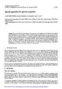
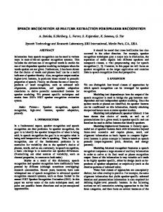
2. DATASETS The CHiME-3 scenario is ASR for a multi-microphone tablet device being used in everyday environments. Four varied environments have been selected: caf´e (CAF), street junction (STR), public transport (BUS) and pedestrian area (PED). For each environment, two types of noisy speech data have been provided, real and simulated. The real data consists of new 6-channel recordings of sentences from the WSJ0 corpus [9] spoken live in the environments. The simulated data was constructed by mixing clean utterances into environment background recordings. Mixing was performed using the techniques described in Section 2.2. For ASR evaluation, the data is divided into official training, development and test sets, details of which are provided in Section 3. 2.1. Real data collection The real data was prepared using the hardware, recording procedures and post-processing described below. 2.1.1. Hardware Recordings have been made using an array of six Audio-technica ATR3350 omnidirectional lavalier microphones mounted in holes drilled through a custom-built frame surrounding a Samsung Galaxy tablet computer. The frame is designed to be held in a landscape orientation and has three microphones spaced both along the top and bottom edges as shown in Figure 1. All microphones face forward (i.e. towards the speaker holding the tablet) apart from the top-center
2
1
3
Companies are listed where transactions generally aggregrate ten thousand shares or one hundred thousand dollars.
4
5
10.0 cm
19.0 cm
6
10.0 cm
Fig. 1: The microphone array geometry. All microphones face forward except for microphone 2.
microphone (mic 2) which faces backwards. The microphone outputs are recorded using a six-channel TASCAM DR-680 portable digital recorder. The channels are sample-synchronized. Speech has also been captured using a Beyerdynamic condenser headset close-talking microphone (CTM). This microphone is recorded using a second TASCAM DR-680 unit that is linked to the first in a master-slave configuration. In this configuration the recorder transports can be started through the master unit interface but the two units are not guaranteed to be precisely synchronized. There was observed to be arbitrary asynchrony between the CTM and the array of ±20 ms across recording sessions. 2.1.2. Recording procedure The recordings have been made by 12 US English talkers (6 male and 6 female) ranging in age from approximately 20 to 50 years old. No talker had any obvious speech impairment and a short test recording was used to screen out talkers who were unable to read aloud with sufficient fluency. Test recordings were made in noisy environments to adjust the TASCAM recording levels to avoid significant clipping. Once set the levels were held constant across all recording sessions. For each talker, recordings were made first in an IAC singlewalled acoustically isolated (but not anechoic) booth (BTH) and then in each of the four noisy target environments. About 100 sentences were read in each location. The talkers used a simple interface that presented WSJ0 prompts on the tablet. It was stressed that each sentence had to be read correctly and without interruption. Talkers were allowed as many attempts as necessary to read each sentence. They were asked to use the tablet in whatever way felt natural and comfortable but they were encouraged to adjust their reading position after each 10 utterances, e.g. either holding the tablet (most typical), resting it on their lap, laying it on a table, etc. Note, the display was fixed in landscape mode. The talker-tablet distance varied but was typically around 40 cm.
the annotator tagged the talker’s most accurate reading of each sentence (typically the last). In cases where even the best rendition contained a reading error, the WSJ0 prompt was edited to produce a corrected transcript (these were typically single word errors occurring in a small fraction of the utterances). Isolated utterances were extracted from the continuous audio according to the annotated start and end times but including 300 ms of padding prior to the utterance (and no post padding). Data was distributed as both continuous audio and as a set of isolated utterances. 2.2. Simulated mixtures The CHiME-3 data is distributed with additional simulated data. These have been constructed by mixing clean speech recordings with noise backgrounds as described below. First, impulse responses (IRs) for the tablet mics are estimated. The microphone signals are represented in the complex-valued short-time Fourier transform (STFT) domain using half-overlapping 256-sample sine windows. The time frames are partitioned into variable-length, half-overlapping and sine-windowed blocks such that the amount of speech is similar in each block. The per-block STFT-domain IRs between the CTM (considered as clean speech) and the other microphones are estimated in the least-squares sense in each frequency bin [10]. IRs are used to estimate the signal-tonoise ratio (SNR) at each tablet mic and, in the case of simulated development or test data, to estimate the noise signal by subtracting the convolved CTM signal. (The estimated tablet mic SNRs had an average of approximately 5 dB). Second, the spatial position of the speaker in the real recordings is tracked using the steered response power phase transform (SRP-PHAT) algorithm [11] (see Section 4.1). The time-varying filter modeling direct sound between the speaker and the microphones is then convolved with a clean speech signal and mixed with a noise signal. In the case of training data, the clean speech signal is taken from the original WSJ0 recordings [9] and it is mixed with a separately recorded noise background. An equalization filter is applied that is estimated as the ratio between the average power spectrum of booth data and that of the original WSJ0 data. In the case of development and test data, the clean speech signal is taken from the booth recordings and it is mixed with the original noisy recording from which speech has been taken out. In either case, the convolved speech signal is rescaled such that the SNR matches that of the original recording. Note, the baseline does not address the simulation of microphone mismatches, microphone failures or reverberation. 3. TASKS Participants are asked to automatically transcribe a set of noisy test recordings and to report the average word error rate (WER) of their system. Systems must be trained using only the provided real and simulated training data. Systems are evaluated on both the real and simulated test sets but with the real test set being used to rank final performance. 3.1. Training and test set definition
2.1.3. Postprocessing Audio recordings were downsampled from 48 kHz to 16 kHz and 16 bits. For each continuous recording session, an annotation file was prepared to record the start and end time of each utterance with a precision of approximately ±100 ms. On a second annotating pass,
The development and test data consists of the same 410 and 330 utterances that make up the corresponding sets in the WSJ0 5k task. For each set the sentences are read by four different talkers in the four CHiME-3 environments. In each environment the set is split into four random partitions and each is assigned to a different talker.
This results in 1640 (410 × 4) and 1320 (330 × 4) real development and test utterances in total. Identically-sized, simulated test sets are made by mixing recordings captured in the recording booth with the backgrounds recovered by subtracting speech from the real recordings (see Section 2.2). The training data consists of 1600 real noisy utterances: four speakers each reading 100 utterances in each of the four environments (i.e. 4 × 4 × 100). These sentences were randomly selected from the 7138 utterance WSJ0 5k training data. The real data is supplemented by 7138 simulated utterances constructed by taking the full WSJ0 5k training set and mixing it into the separately recorded CHiME-3 noise backgrounds, again, as described in Section 2.2. 3.2. Additional instructions A set of challenge ‘rules’ were provided to participants. The rules were designed to keep systems close to the application scenario and to make systems more directly comparable. The key rules were as follows. It was stated that participants should not extend the training data. However, to allow benefit from improved simulation, participants were allowed to construct modified versions of the simulated training data under the constraint that they keep the same pairing between utterances and segments of noise background. It was allowed that the language model could be changed, but that all language models must be trained solely from the official WSJ language model training data. Participants were disallowed from using the test utterance environment labels. A constraint of 5 seconds was placed on the amount of audio preceding the utterance that could be used at test time. All parameters had to be tuned using just the official training and development data, and that systems should be run (ideally just once) on the final test set using the parameter settings suggested by the development data. If participants wished to extend their research beyond the rules, they were asked to present results of both their best compliant and noncompliant systems. 4. BASELINES Participants were provided with baseline systems for front-end signal enhancement (MATLAB based) and state-of-the art GMM/DNN based ASR (using the Kaldi toolkit). 4.1. Enhancement The speech enhancement baseline aims to transform the multichannel noisy input signal into a single-channel enhanced output signal suitable for ASR processing. The signals are represented in the complex-valued STFT domain using half-overlapping sine windows of 1024 samples. The spatial position of the target speaker in each time frame is encoded by a nonlinear SRP-PHAT pseudo-spectrum [12], which was found to perform best among a variety of source localization techniques [13]. The peaks of the SRP-PHAT pseudo-spectrum are then tracked over time using the Viterbi algorithm. The transition probabilities between successive speaker positions are inversely related to their distance and to the distance to the center of the microphone array. The multichannel covariance matrix of noise is estimated from 400 ms to 800 ms of context immediately before the test utterance (i.e. making use of the known utterance start time). The speech signal is then estimated by time-varying minimum variance distortionless response (MVDR) beamforming with diagonal loading [14], taking possible microphone failures into account. The full 5 s of
allowed context are not used since they often contain unannotated speech. 4.2. GMM baseline The baseline acoustic features are MFCCs (13 order). Three frames of left and right context are concatenated to form a 91-dimensional feature vector which is compressed to 40 dimensions using linear discriminative analysis (LDA) whose class is one of 2500 tied triphone HMM states. The tied states are modeled by a total of 15,000 Gaussians. maximum likelihood linear transformation (MLLT), and feature-space maximum likelihood linear regression (fMLLR) with speaker adaptive training (SAT) are also applied. The effectiveness of these feature transformation techniques for distant talk speech recognition was shown in [15]. This first baseline is designed to provide a competitive score at relatively low computational cost, therefore, advanced processing techniques requiring a heavy cost (e.g., discriminative training) are not included. 4.3. DNN baseline The deep neural network (DNN) baseline provides the state-of-theart ASR performance. It is based on the Kaldi recipe for Track 2 of the 2nd CHiME Challenge [16]. The DNN has 7 layers with 2048 units per hidden layer. The input layer has 5 frames of left and right context (i.e. 11 × 40 = 440 units). The DNN is trained using the standard procedure: pre-training using restricted Boltzmann machines, cross entropy training, and sequence discriminative training using the state-level minimum Bayes risk (sMBR) criterion [17]. This second baseline requires a much greater computational resource (GPUs for the DNN training and many CPUs for lattice generation) but provides a significant increase in recognition performance. 4.4. Baseline performance Baseline system performance is summarized in Tables 1 and 2. Considering Table 1, the first two rows show that training on the real and simulated noisy speech dramatically reduces the WER with respect to training on the mismatched clean speech. For the development data, the simulated test data produces the same 18.7% WER as the real test data. In rows three and four it is seen that the baseline enhancement reduces the mismatch between the noisy data and clean training data. However, when training and testing on enhanced data, the simulated test set WER is reduced from 21.6% down to 10.6% but the real data performance actually gets worse, with a WER increasing from 33.2% to 37.4%. This is likely to be because the enhancement strategy works better on the simulated data than on the real data, so after enhancement the simulated portion of the training data is not well matched to the real test data. The last two rows show the results for the full DNN baseline which on the development data provides a further 3% absolute WER reduction but which does not provide simalar improvements in the test data. It can be seen that, for the real data, the WERs on the evaluation test set are nearly twice as large as those on the development set. This was surprising as there was no obvious mismatch in the recording conditions. Closer analysis showed that increased WERs were seen across all environments and also when using the CTM recordings. This suggests that it is likely to be a speaker effect rather than than an environment effect. Indeed, of the four evaluation set speakers, one produced WERs in the same range as the development set speakers, while the other three appeared to have particularly challenging speaking styles.
Table 1: WERs for the GMM and DNN baseline systems for both the real and simulated, development and test sets. Models are trained on either clean, noisy or enhanced noisy data and tested either before or after enhancement. Enhancement combines all 6 channels, other results use only channel 5 (similar scores were achieved for all forward facing mics; performance is poorer on the rear facing mic 2.) Model
Test noisy
GMM enh. DNN
noisy enh.
Train clean noisy clean enh. noisy enh.
Dev. Real 55.7 18.7 41.9 20.6 16.1 17.7
data Sim. 50.3 18.7 21.7 9.8 14.3 8.2
Test data Real Sim. 79.8 63.3 33.2 21.6 78.1 25.6 37.4 10.6 33.4 21.5 33.8 11.2
Table 2: WER by environment for DNN system trained on noisy data. Corresponds to highlighted row in Table 1. Environment BUS CAF PED STR
Dev. Real 23.5 13.8 11.4 15.8
data Sim. 14.6 17.5 11.2 13.9
Test data Real Sim. 51.8 20.6 34.7 23.8 27.2 21.7 20.1 19.9
Table 2 shows a breakdown of the best development set result by environment. In both the development and test sets the highest WER is scene in the BUS environment. This is surprising considering that the noise background in the bus is often quite stationary. There are two possible reasons for the poor performance. First, when traveling on a bus there is a lot of vibration and acceleration. It is often hard for the talker to hold the tablet steady and so their is more apparent talker motion observed in the microphone signals. Second, compared to when talking in a caf´e or an open public area, talkers tended to adopt a quieter style of talking so as not to be overheard or to disturb fellow passengers. 5. SUBMITTED SYSTEMS 26 teams participated in the challenge. The teams were mainly from Asia, Europe and North America and represented a mix of industry and academia. It is notable that many of the teams were large and involved collaboration across multiple institution or multiple research groups within institutions. Teams typically employed multiple strategies implemented by improving or replacing components in the processing pipeline of the baseline systems. The strategies employed by each team are summarised under eight headings in Table 3. In the sections below these strategies are discussed under four broad headings: target enhancement, feature design, statistical modeling and training methods/data. 5.1. Target enhancement Performing good target enhancement, prior to feature extraction, is crucial for good performance, and nearly all teams have attempted to improve this component of the baseline system. Enhancement is achieved through a mixture of multi-channel processing that exploits spatial diversity and single channel approaches that exploit differences in the spectral properties of the speech and noise (columns Mult.Ch.Enh. and Sing.Ch.Enh. in Table 3, respectively).
Many systems improved performance by replacing the baseline system’s super-directive MVDR beamformer with a conventional delay and sum beamformer, e.g. [19, 21, 33]. Others had success in improving the MVDR, for example by applying a timefrequency mask during estimation of the steering vector [18]. [27] make the necessary speech and noise covariance estimates using a DNN. Commonly, beamformers have been complemented with post-filtering stages, for example spatial coherence filtering [32, 41] or filtering to achieve dereverberation [18, 40]. In [21] a DNN estimates the power spectral density (PSD) of speech from a single channel which is then used to estimate the spatial covariance matrices for speech and noise needed in the multichannel processing. In [29] several beamforming strategies are employed and successfully combined at the lattice level during decoding. Purely single channel approaches, i.e. fully decoupled from the multichannel processing, have been less commonly applied and have had mixed success: [39] and [25] use NMF-based source separation approaches that exploit the sparseness of spectral representations and the diversity between speech and noise spectra, whereas [23] employs a separation technique that tracks noise using minimum statistics. Deep learning approaches have also been employed: [19] use a bidirectional Long Short-Term Memory (BLSTM) for time-frequency mask estimation; [34] and [40] use DNN and BLSTM-based denoising autoencoders respectively; [35] attempts DNN-based mask estimation using pitch-based features but fails to demonstrate WER reductions. 5.2. Feature design The references system employs Mel-frequency cepstral coefficient (MFCC) features for initial GMM/HMM alignment and then filterbank features for the DNN pass. Most systems inherited the same basic design but used different features for the DNN stage, and added techniques to better normalize across speaker and noise variation. In [23, 24], DNN filterbank features have been supplemented by delta and delta-delta features. [24] shows that this provides a significant improvement despite the 11 frames of context being employed by the DNN stage. A few teams have employed auditory-like representations to augment or replace the reference Mel-filterbank. [20, 35] use a Gammatone filterbank that has broader filter tails and has been shown to provide noise robustness. Four systems have used amplitude modulation-based features either by applying a discrete cosine transform (DCT) on the filterbank envelopes [37]; employing a 2D Gabor filter bank [22]; or tracking amplitude modulation (AM) in filterbands using a non-linear Teager energy operator [19]. In place of filterbank features, [26] claim better performance using MFCC-based features, and [21, 30] employ perceptual linear prediction (PLP)-based features. Unfortunately, there are no experiments making a direct comparison. More typically, where alternative features have been used they have been combined with filterbank features either at the feature-level (e.g. [20]) or, more commonly, after decoding using lattice combination approaches. The most significant gains have been achieved by using techniques to improve the speaker-invariance of the DNN stage. The simplest approach has been to apply utterance-based feature mean and variance normalization [20, 23, 24, 28]. A small amount of speaker invariance can also be gained by augmenting DNN features with pitch-based features [20, 28, 35]. However, the two most effective techniques are transforming the DNN features using fMLLR [19, 21, 22, 25, 26] or augmentation of the DNN features using either i-vectors (e.g. [22, 30]), or bottleneck features [31],
Yoshioka et al. [18] Hori et al. [19] Du et al. [20] Sivasankaran et al. [21] Moritz et al. [22] Fujita et al. [23] Zhao et al. [24] Vu et al. [25] Tran et al. [26] Heymann et al. [27] Wang et al. [28] Jalalvand et al. [29] Zhuang et al. [30] Tachioka et al. [31] Pang and Zhu [32] Prudnikov et al. [33] Bagchi et al. [34] Ma et al. [35] Pertila et al. [36] Castro Martinez et al. [37] Pfeifenberger et al. [38] Baby et al. [39] Mousa et al. [40] Barfuss et al. [41] Misbullah et al. [42] DNN Baseline
!
! ! ! ! ! ! ! ! ! ! ! ! !
i.e. extracted from bottleneck layers in speaker classification DNNs. Where i-vectors have been used they may be either per-speaker, e.g. [33], or per-speaker-environment, e.g [35]. Many teams have used both fMLLR and i-vectors/bottleneck features [30–33]. It should be noted that all these techniques will also normalizing environment variation to some extent. 5.3. Statistical modeling Systems have been separately analyzed in terms of their approach to acoustic modeling and language modeling. For acoustic modeling, the majority of teams adopted the DNN architecture supplied by the baseline system. Of the alternative architectures explored the most common were convolutional neural networkss (CNNs) (e.g. [18, 28, 30, 35, 39]) and forms of Long Short Time Memory (LSTM) networks (e.g. [20, 28, 30, 32, 39, 42]). [42] uniquely employs deep networks built from alternating LSTM and feedfoward layers. [18] employs a convolutional network scheme known as ‘network in network’ adopted from the vision community that alternates convolutional layers with fully-connected feed forward layers. Several teams combined multiple architectures [18,
System Comb.
Lang. Model
Acoust. Model
! ! ! ! ! ! ! ! ! ! ! ! ! ! ! ! ! ! ! ! ! !
Feature Trans.
Feature Extract.
! ! ! ! ! ! ! ! ! ! ! ! ! ! ! ! ! ! ! ! ! ! ! ! ! ! ! !
Sing. Ch. Enh.
Mult. Ch. Enh.
System
Training
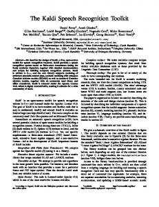
Table 3: Overview of the 26 systems submitted to the CHiME-3 Challenge. The left side of the table summarizes the key features of each system. Ticks indicate where the systems differ significantly from the baseline DNN system that was provided. The right hand side summarises the system performances. Systems are ranked according to their performance on the real data evaluation test set. All figures represent percentage WERs. Average WERs are shown for both the simulated data (Sim) and the real data evaluation sets. Results for the real data are further broken down by environment.
! ! ! ! ! ! ! ! ! ! ! ! ! ! ! ! ! ! ! ! ! ! ! ! ! ! !
! !
Sim Ave. 4.5 8.6 7.0 6.2 6.4 9.8 8.2 8.5 8.6 9.0 9.7 7.1 6.2 8.4 6.1 13.8 21.0 20.0 24.4 15.9 14.9 6.9 21.5 15.2 16.9 21.5
BUS 7.4 13.5 13.8 16.2 13.5 16.6 14.5 17.6 18.6 17.5 17.7 17.7 18.0 23.2 16.2 17.4 24.7 24.6 28.4 30.5 29.0 28.4 30.7 35.6 45.0 51.8
CAF 4.5 7.7 11.4 9.6 13.5 11.8 11.7 12.1 10.7 10.5 11.8 14.1 15.4 13.9 13.4 11.5 14.0 18.4 20.6 23.8 24.0 26.5 27.3 32.7 29.2 34.7
Real Data PED 6.2 7.1 9.3 12.3 10.6 10.0 11.5 8.5 9.7 11.0 13.4 13.0 12.2 11.1 17.0 18.0 13.7 16.9 19.0 18.1 19.8 22.3 21.3 26.6 23.8 27.2
STR 5.2 8.1 7.8 7.2 9.2 8.8 10.0 9.6 9.6 10.0 10.0 9.2 9.6 8.4 10.5 10.5 12.9 14.4 16.4 15.5 15.7 15.1 18.3 19.9 19.1 20.1
Ave. 5.8 9.1 10.6 11.3 11.7 11.8 11.9 11.9 12.1 12.3 13.2 13.5 13.8 14.2 14.3 14.3 16.3 18.6 21.1 22.0 22.1 23.1 24.4 28.7 29.3 33.4
20,30]. Performance benefits of the various architectures remain unclear, however it is notable that some of the best scoring systems have used the baseline DNN configuration. Nearly half the teams chose to employ some form of language model rescoring to improve performance of the baseline 3-gram model. This step was taken by most of the top scoring teams and appears to have been important for success. Rescoring was performed using either a DNN-LM [25], LSTM-LM [40] or most commonly an recurrent neural network language model (RNN-LM) [18,21,31,38]. Some teams using RNN-LM rescoring also increased the context of the 3-gram model, replacing it with a 4-gram [29,32] or 5-gram [19]. Teams have trained the RNN-LM on carefully selected subsets of the complete WSJ training data, e.g. [18]. [29] selects training material fitted to the transcripts produced by the first pass 3-gram decoding. Most teams ran experiments using multiple enhancement, feature extraction and statistical modeling techniques. About half the teams exploited the complementarity between competing approaches by by employing lattice-based hypothesis combination techniques (see final column of Table 3). Other teams, including the overall top scorer [18], combined classifiers using multi-pass cross-adaptation techniques.
In order to encourage teams to explore techniques for data simulation, the challenge rules allowed teams to remix the simulated training data. In the event, few teams took advantage of this: [27] and [28] obtained consistent performance improvements by expanding the training set by remixing each training utterance at different SNRs. [21] generated simulated training data in the feature domain by sampling from a conditional RBM, but the technique failed to improve results. Other teams trained systems on all the individual channels rather than on a single enhanced signal [18, 22, 24, 30]. Surprisingly, this often proved to be effective despite the mismatch between non-enhanced training signals and enhanced test data. One team employed a semi-supervised training technique, i.e. adapting the DNN using the labels that had been estimated on the complete test set in a first pass through the data [26]. 6. SUMMARY OF RESULTS Results for all 26 systems are shown in Table 3. Systems are ranked according to their average WER on the real test data. All systems have improved upon the baseline WER of 33.4% with most systems reporting WERs in the range 11-15%. The top-ranked system, Yoshioka et al. [18], has a WER of 5.83%, significantly lower than that of all others. Comparing WERs across environments, some clear patterns emerge. Nearly all systems have highest WERs in the bus environment (BUS) and all but four have lowest WERs in the street (STR). However, it is striking that the two top systems are unique in having performed best in the caf´e environment (CAF). This suggests that these systems have greater robustness to the competing speech and the non-stationary backgrounds that characterize the caf´e setting. Although it is hard to draw robust conclusions from crosssystem comparisons, a number of observation can be made from the distribution of ticks in the table. First, it is clear that there is no single technique that is sufficient for success. Systems that have concentrated on just one or two components have done consistently poorly. Generally, there are more ticks at the top of the table, i.e. each improved component has led to some incremental performance boost. Nearly all teams have gained performance by optimizing the multichannel enhancement. However, the top systems are distinct in that they have also added feature normalization to the DNN stage and employed some form of language model rescoring. ROVER-style system combination is used by the 2nd, 3rd and 4th placed team, but does not seem necessary for top performance: system combination through good engineering is perhaps preferable. The overall best system [18] has combined classifiers using a sophisticated cross-adaptation approach. 7. DISCUSSION A secondary objective of the CHiME-3 challenge has been to examine the role of artificially mixed speech data in noise-robust ASR evaluation. We will consider this question from two separate perspectives: simulation for training and simulation for evaluation. The attraction of simulated training data is that it is cheap to construct and that it supports techniques which can exploit stereo pairing between noisy and clean signals. The Challenge provided a small amount of real data but a larger amount of simulated data that teams could ignore or exploit. Rules also allowed for participants to improve the simulation algorithms and either replace or augment
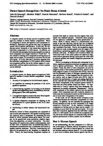
WER on simulated evaluation data
5.4. Training methods and data
WER on real evaluation data
Fig. 2: WER on simulated versus real data across all systems.
the training set. It was observed that all the best performing systems found value in the simulated data for acoustic model training. However, some care was needed in using simulated data to tune the microphone array processing. Broadly speaking the baseline simulation techniques employed do not sufficiently capture the full complexity of the real array data. Fitting to the simulated data may lead to sub-optimal results for real array processing, or overly enhanced simulated data that causes mismatch when training acoustic models. Next we consider the value of simulated data for system testing. The value of simulation for evaluation is less clear, i.e. evaluation sets are smaller and therefore cheaper to collect; unmixed ground truth is not strictly required. However, given the number of previous challenges using simulated evaluations (include CHiME-1 and CHiME-2) it is of interest to ask whether performance on simulated evaluation data is predictive of performance on real data? Figure 2 shows a plot of the WER for the simulated evaluation set plotted against that for the real data set for all 26 CHiME-3 systems. Although, there appears to be a strong correlation, there are many outlying systems for which simulated data performance would give an extremely over-optimistic estimate of real performance, e.g. Baby et al. [39]. Further, within the large cluster of systems with simulated data WERs between 6% and 10% , there is no significant correlation between the scores. Note, participants were not allowed to produce separately tuned systems for both data sets, but were told that systems would be ranked on the real data. It can be assumed that participants have therefore optimized performance for the real data. It remains unclear whether the above observations would remain true if optimizing performance on the simulated set, e.g. as in previous evaluations. 8. CONCLUSIONS The CHiME-3 challenge has used the WSJ 5k task to evaluate multimicrophone ASR in noisy settings with talker-microphone distances of ∼40 cm. This relatively simple task has highlighted the importance of carefully engineered multi-channel enhancement and statistical modeling. Most teams failed to get WERs below 10% and most systems required complex multi-pass strategies that may not be practical in real applications. However, the best system achieved a WER of 5.83%, comparable with the best WSJ scores previously reported for clean speech. Research should now focus on moving to larger talker-microphone distances and using less constrained speech tasks. The challenge has drawn attention to the value of simulated training data, but highlighted the need for better simulation algorithms. It has also demonstrated that caution is needed when interpreting results of challenges that use simulated evaluation data.
9. REFERENCES [1] “RWCP meeting speech corpus (RWCP-SP01),” 2001. [2] D. Mostefa, N. Moreau, K. Choukri, G. Potamianos, S. M. Chu, A. Tyagi, J. R. Casas, J. Turmo, L. Cristoforetti, F. Tobia, et al., “The CHIL audiovisual corpus for lecture and meeting analysis inside smart rooms,” Language Resources and Evaluation, vol. 41, no. 3-4, pp. 389–407, 2007. [3] S. Renals, T. Hain, and H. Bourlard, “Interpretation of multiparty meetings: The AMI and AMIDA projects,” in Proceedings of the 2nd Joint Workshop on Hands-free Speech Communication and Microphone Arrays (HSCMA), 2008, pp. 115– 118. [4] M. Lincoln, I. McCowan, J. Vepa, and H. Maganti, “The multichannel Wall Street Journal audio visual corpus (MC-WSJAV): specification and initial experiments,” in Proceedings of the 2005 IEEE Workshop on Automatic Speech Recognition and Understanding (ASRU), 2005, pp. 357–362. [5] H.-G. Hirsch and D. Pearce, “The Aurora experimental framework for the performance evaluation of speech recognition systems under noisy conditions,” in Proceedings of the 6th International Conference on Spoken Language Processing (ICSLP), 2000, vol. 4, pp. 29–32. [6] N. Parihar, J. Picone, D. Pearce, and H. G. Hirsch, “Performance analysis of the Aurora large vocabulary baseline system,” in Proceedings of the 2004 European Signal Processing Conference (EUSIPCO), Vienna, Austria, 2004, pp. 553—556. [7] J. Segura, T. Ehrette, A. Potamianos, D. Fohr, I. Illina, P. Breton, V. Clot, R. Gemello, M. Matassoni, and P. Maragos, “The HIWIRE database, a noisy and non-native English speech corpus for cockpit communication,” Online. http://www. hiwire. org, 2007. [8] A. Brutti, L. Cristoforetti, W. Kellermann, L. Marquardt, and M. Omologo, “WOZ acoustic data collection for interactive TV,” Language Resources and Evaluation, vol. 44, no. 3, pp. 205–219, 2010. [9] J. Garofalo, D. Graff, D. Paul, and D. Pallett, “CSR-I (WSJ0) Complete,” Linguistic Data Consortium, Philadelphia, 2007. [10] E. Vincent, R. Gribonval, and M. Plumbley, “Oracle estimators for the benchmarking of source separation algorithms,” Signal Processing, vol. 87, no. 8, pp. 1933–1059, 2007. [11] J. DiBiase, H. Silverman, and M. Brandstein, “Robust localization in reverberant rooms,” in Microphone arrays: signal processing techniques and applications, M. Brandstein and D. Ward, Eds., chapter 8, pp. 157–180. Springer-Verlag, 2001. [12] B. Loesch and B. Yang, “Adaptive segmentation and separation of determined convolutive mixtures under dynamic conditions,” in Proceedings of the 9th International Conference on Latent Variable Analysis and Signal Separation (LVA/ICA), 2010, pp. 41–48. [13] C. Blandin, A. Ozerov, and E. Vincent, “Multi-source TDOA estimation in reverberant audio using angular spectra and clustering,” Signal Processing, vol. 92, no. 8, pp. 1950–1960, 2012. [14] X. Mestre and M. A. Lagunas, “On diagonal loading for minimum variance beamformers,” in Proceedings of the 3rd IEEE International Symposium on Signal Processing and Information Technology (ISSPIT), 2003, pp. 459–462.
[15] Y. Tachioka, S. Watanabe, J. Le Roux, and J. R. Hershey, “Discriminative methods for noise robust speech recognition: A CHiME challenge benchmark,” in Proceedings of the 2nd International Workshop on Machine Listening in Multisource Environments (CHiME), 2013, pp. 19–24. [16] C. Weng, D. Yu, S. Watanabe, and B.-H. F. Juang, “Recurrent deep neural networks for robust speech recognition,” in Proceedings of the 2014 IEEE International Conference on Acoustics, Speech, and Signal Processing (ICASSP), 2014, pp. 5532– 5536. [17] K. Vesel´y, A. Ghoshal, L. Burget, and D. Povey, “Sequencediscriminative training of deep neural networks,” in Proceedings of the 14th Annual Conference of the International Speech Communication Association (INTERSPEECH 2013), 2013, pp. 2345–2349. [18] T. Yoshioka, N. Ito, M. Delcroix, A. Ogawa, K. Kinoshita, M. F. C. Yu, W. J. Fabian, M. Espi, T. Higuchi, S. Araki, and T. Nakatani, “The NTT CHiME-3 system: Advances in speech enhancement and recognition for mobile multi-microphone devices,” in Proc. IEEE ASRU, 2015. [19] T. Hori, Z. Chen, H. Erdogan, J. R. Hershey, J. L. Roux, V. Mitra, and S. Watanabe, “The MERL/SRI system for the 3rd CHiME challenge using beamforming, robust feature extraction, and advanced speech recognition,” in Proc. IEEE ASRU, 2015. [20] J. Du, Q. Wang, Y.-H. Tu, X. Bao, L.-R. Dai, and C.-H. Lee, “An information fusion approach to recognizing microphone array speech in the CHiME-3 challenge based on a deep learning framework,” in Proc. IEEE ASRU, 2015. [21] S. Sivasankaran, A. A. Nugraha, E. Vincent, J. A. MoralesCordovilla, S. Dalmia, and I. Illina, “Robust ASR using neural network based speech enhancement and feature simulation,” in Proc. IEEE ASRU, 2015. [22] N. Moritz, S. Gerlach, K. Adiloglu, J. Anem¨uller, B. Kollmeier, and S. Goetze, “A CHiME-3 challenge system: Long-term acoustic features for noise robust automatic speech recognition,” in Proc. IEEE ASRU, 2015. [23] Y. Fujita, R. Takashima, T. Homma, R. Ikeshita, Y. Kawaguchi, T. Sumiyoshi, T. Endo, and M. Togami, “Unified ASR system using LGM-based source separation, noise-robust feature extraction, and word hypothesis selection,” in Proc. IEEE ASRU, 2015. [24] S. Zhao, X. Xiao, Z. Zhang, T. N. T. Nguyen, X. Zhong, B. Ren, L. Wang, D. L. Jones, E. S. Chng, and H. Li, “Robust speech recognition using beamforming with adaptive microphone gains and multichannel noise reduction,” in Proc. IEEE ASRU, 2015. [25] T. T. Vu, B. Bigot, and E. S. Chng, “Speech enhancement using beamforming and non negative matrix factorization for robust speech recognition in the CHiME-3 challenge,” in Proc. IEEE ASRU, 2015. [26] H. D. Tran, J. Dennis, and L. Yiren, “A comparative study of multi-channel processing methods for noisy automatic speech recognition on the third CHiME challenge,” Submitted to 2016 IEEE International Conference on Acoustics, Speech, and Signal Processing (ICASSP). [27] J. Heymann, L. Drude, A. Chinaev, and R. Haeb-Umbach, “BLSTM supported GEV beamformer front-end for the 3rd CHiME challenge,” in Proc. IEEE ASRU, 2015.
[28] X. Wang, C. Wu, P. Zhang, Z. Wang, Y. Liu, X. Li, Q. Fu, and Y. Yan, “Noise robust ioa/cas speech separation and recognition system for the third ’chime’ challenge,” 2015, arXiv:1509.06103. [29] S. Jalalvand, D. Falavigna, M. Matassoni, P. Svaizer, and M. Omologo, “Boosted acoustic model learning and hypotheses rescoring on the CHiME3 task,” in Proc. IEEE ASRU, 2015. [30] Y. Zhuang1, Y. You, T. Tan, M. Bi, S. Bu, W. Deng, Y. Qian, M. Yin, and K. Yu1, “System combination for multi-channel noise robust ASR,” Tech. Rep. SJTU SpeechLab Technical Report, SP2015-07, Department of Computer Science and Engineering, Shanghai Jiao Tong University, Shanghai, China, 2015. [31] Y. Tachioka, H. Kanagawa, and J. Ishii, “The overview of the MELCO ASR system for the third CHiME challenge,” Tech. Rep. SVAN154551, Mitsubishi Electric, 2015. [32] Z. Pang and F. Zhu, “Noise-robust asr for the third ’chime’ challenge exploiting time-frequency masking based multichannel speech enhancement and recurrent neural network,” 2015, arXiv:1509.07211. [33] A. Prudnikov, M. Korenevsky, and S. Aleinik, “Adaptive beamforming and adaptive training of DNN acoustic models for enhanced multichannel noisy speech recognition,” in Proc. IEEE ASRU, 2015. [34] D. Bagchi, M. I. Mandel, Z. Wang, Y. He, A. Plummer, and E. Fosler-Lussier, “Combining spectral feature mapping and multi-channel model-based source separation for noise-robust automatic speech recognition,” in Proc. IEEE ASRU, 2015. [35] N. Ma, R. Marxer, J. Barker, and G. J. Brown, “Exploiting synchrony spectra and deep neural networks for noise-robust automatic speech recognition,” in Proc. IEEE ASRU, 2015. [36] P. Pertila, A. Hurmalainen, S. Nandakumar, and T. Virtanen, “Automatic speech recognition with multichannel neural network based speech enhancement,” Tech. Rep. ISBN 978-95215-3590-1, Department of Signal Processing, Tampere University of Technology, 2015. [37] A. C. Martinez and B. Meyer, “Mutual benefits of auditory spectro-temporal Gabor features and deep learning for the 3rd CHiME challenge,” Tech. Rep. Techncial Report 2509, University of Oldenburg, Germany, 2015, url:http://oops.unioldenburg.de/2509. [38] L. Pfeifenberger, T. Schrank, M. Z¨ohrer, M. Hagm¨uller, and F. Pernkopf, “Multi-channel speech processing architectures for noise robust speech recognition: 3rd CHiME challenge results,” in Proc. IEEE ASRU, 2015. [39] D. Baby, T. Virtanen, and H. V. hamme, “Coupled dictionarybased speech enhancement for CHiME-3 challenge,” Tech. Rep. KUL/ESAT/PSI/1503, KU Leuven, ESAT, Leuven, Belgium, Sept. 2015. [40] A. E.-D. Mousa, E. Marchi, and B. Schuller, “The ICSTM+TUM+UP approach to the 3rd CHiME challenge: Single-channel LSTM speech enhancement with multi-channel correlation shaping dereverberation and LSTM language models,” 2015, arXiv:1510.00268. [41] H. Barfuss, C. Huemmer, A. Schwarz, and W. Kellermann, “Robust coherence-based spectral enhancement for distant speech recognition,” 2015, arXiv:1509.06882.
[42] A. Misbullah and J.-T. Chien, “Deep feedforward and recurrent neural networks for speech recognition,” unpublished technical report.