The solution of a boundary value problem is commonly obtained by sep- aration of variables. In a particular unbounded coordinate, the solution is usually.
THE TRUNCATED REGION EIGENFUNCTION EXPANSION METHOD FOR THE SOLUTION OF BOUNDARY VALUE PROBLEMS IN EDDY CURRENT NONDESTRUCTIVE EVALUATION Theodoros. P. Theodoulidis and John R. Bowler Iowa State University, Center for Nondestructive Evaluation, 1915 Scholl Road, Ames, IA 50011 ABSTRACT. A number of complex problems in eddy current nondestructive evaluation have been solved recently using the truncated region eigenfunction expansion method. The solution of a boundary value problem is commonly obtained by separation of variables. In a particular unbounded coordinate, the solution is usually expressed as an integral form such as a Fourier or Bessel integral. However, by truncating the domain of the problem, a modified solution is obtained in the form of a series expansion instead of an integral. Although one achieves a gain in computation efficiency in this way, the most significant advantage of the approach is the ability to match interface conditions across several boundaries simultaneously and thus obtain analytical solutions to complex problems. We illustrate the approach by solving the axisymmetric, time harmonic boundary value problem of a coil above a coaxial hole in a plate.
INTRODUCTION In the last two years we have been studying various eddy current canonical problems with the TREE method where the acronym stands for Truncated Region Eigenfunction Expansion. As in the classical approach, the method uses separation of variables to express the electromagnetic field in the various regions of the problem in analytical form. It differs from the classical approach in truncating the solution domain to limit the range of a coordinate that would otherwise have an infinite span. As a result, the solution dependence on that coordinate is expressed as a series form, rather than as an integral. There are a number of advantages of recasting the expressions as sums rather than integrals. For example, the numerical implementation is usually more efficient and error control easier, but these are secondary issues. The main advantage of the truncated domain option is that by a careful selection of the discrete eigenvalues and the corresponding eigenfunctions, the field continuity can be satisfied at various interfaces simultaneously. In this way, the class of problems that can be treated analytically is greatly extended. The matching of the field expressions at interfaces is done either on a term by term basis or by mode matching where the testing functions are the same as the expansion functions. The latter implies that the TREE method may contain a meshless Galerkin type procedure with expansion and testing functions that are entire domain functions. At the same time, the functions satisfy the electromagnetic field equations. This is not a numerical method though since the resultant field is an analytical solution of the governing 1 CP760, Review of Quantitative Nondestructive Evaluation Vol. 24, ed. by D. O. Thompson and D. E. Chimenti © 2005 American Institute of Physics 0-7354-0245-0/05/$22.50
403
equations. On the other hand it is not strictly analytical because it requires the numerical inversion of a full matrix as well as the numerical computation of the discrete eigenvalues. Taking into account these facts, we describe the method as quasi-analytical. The following is a list of canonical problems that have been solved or are currently under investigation: • Long crack in a uniform field (TE 2D) [1]. • Long coil above an edge or above a long slot/crack (TM 2D) [2]. • Ferrite-cored coil with cylindrical [3] or E-shaped core above a layered half-space (Axi2D). • Finite length conductive rod and encircling coil (Axi-2D) [4]. • Coil in or above hole in a conductive space (Axi-2D and 3D). • Coil in a tube (Axi-2D and 3D): end effect [5] axisymmetric grooves and deposits, inside or outside diameter support plates WF-NDE benchmark problem (Problem 1 - Axisymmetric) • Coil above an edge - The corner conductor problem (3D) [6]. • Coil above a long slot/crack (3D). In the above list, the type of the problem is indicated in parenthesis as a two-dimensional (2D), three-dimensional (3D), axisymmetric (Axi), transverse electric (TE) or transverse magnetic (TM). The TREE method has also been used in a reformulation of the classical Dodd an Deeds models [7], where the integral expressions are replaced by series. The various advantages of this approach are discussed in [8]. FORMULATION In this article, we consider the axisymmetric eddy current problem of a coil over a plate with a cylindrical hole as shown in Fig. 1. This is a first step towards the development of a theory of eddy current inspection of fastener holes in aircraft structures. The plate is non-magnetic (µr = 1) having a conductivity σ and thickness d. The electromagnetic field is represented in a cylindrical coordinate system by a magnetic vector potential having only an azimuthal component Aφ (r, z). In a nonconducting region, the potential satisfies the Laplace equation and in the conductor, the Helmholtz equation. First we consider a filamentary source coil, assume a harmonic current excitation varying as the real part of Iejωt and subdivide the problem domain into four regions, Fig.1a. The solution domain is truncated at a radius r = h and we proceed by expanding the magnetic vector potential Aφ in a series of eigenfunctions satisfying a homogeneous Dirichlet condition at this boundary: Aφ (h, z) = 0. The expressions for Aφ in the four regions of the problem, Fig.1a, are written in the following form: A1 (r, z) =
∞ X
J1 (ui r)e−ui z D1i
(1)
i=1
A2 (r, z) =
∞ X
h
J1 (ui r) eui z C2i + e−ui z D2i
i=1
404
2
i
(2)
zr
Aö=0
zr
Aö=0
Aö=0
r2
r0
(1)
Aö=0
r1 z2
z0
(2)
z1
z=0
z=0
(3) z=-d
c
h
h
(4)
z=-d
c
(a)
(b)
FIGURE 1. Axisymmetric view of (a) filamentary and (b) rectangular cross-section coil above a conductive plate with a coaxial hole.
∞ P [Y1 (qi h)J1 (qi c) − J1 (qi h)Y1 (qi c)] J1 (pi r) [epi z C3i + e−pi z D3i ]
A3 (r, z) = i=1 ∞ P
and
i=1
0≤r≤c
J1 (pi c) [Y1 (qi h)J1 (qi r) − J1 (qi h)Y1 (qi r)] [epi z C3i + e−pi z D3i ] c ≤ r ≤ h, (3) A4 (r, z) =
∞ X
J1 (ui r)eui z C4i ,
(4)
i=1
where J1 , Y1 are Bessel functions and Cν,i , and Dν,i ν = 1, 2, 3, 4 are expansion coefficients. Only the C2i are known a priori, since they are deduced using the same source in the absence of the plate. The eigenvalues of the full problem are ui pi and qi where p2i = qi2 + jωµ0 σ. After truncating to Ns terms, the above expressions are rewritten using matrix notation: A1 (r, z) = J1 (uT r)e−uz D1 . T
In (5), J1 (u r) is a 1 × Ns vector, e unknown coefficients: A1 (r, z) = J1 (uT r)e−uz D1 =
h
−uz
(5)
is a Ns × Ns matrix and D1 is a Ns × 1 vector of
i J1 (u1 r) J1 (u2 r) · · ·
e−u1 z 0 0 e−u2 z 0
0
0 D1,1 0 D1,2 . (6) . ... ..
Similarly for the remaining regions h
i
A2 (r, z) = J1 (uT r) euz C2 + e−uz D2 , A3 (r, z) =
(
J1 (pT r) [Y1 (qc)J1 (qh) − J1 (qc)Y1 (qh)] [epz C3 + e−pz D3 ] [Y1 (qc)J1 (qh) − J1 (qc)Y1 (qh)]T J1 (pr) [epz C3 + e−pz D3 ]
(7) 0≤r≤c , c≤r≤h
(8)
and A4 (r, z) = J1 (uT r)euz C4 .
(9)
The eigenfunctions and corresponding eigenvalues in (1)-(9) are selected to satisfy boundary and interface conditions. Here, the ui eigenvalues are easily computed from the equation J1 (ui h) = 0 405
3
(10)
implied by the condition Aφ (h, z) = 0. The complex eigenvalues of the problem, pi and qi , which are related by p2i = qi2 + jωµ0 σ, are computed from the roots of the equation qi J1 (pi c)[Y1 (qi h)J0 (qi c) − J1 (qi h)Y0 (qi c)] = pi J0 (pi c)[Y1 (qi h)J1 (qi c) − J1 (qi h)Y1 (qi c)],
(11)
derived from (8) by enforcing the continuity of the tangential magnetic field at r = c. The unknown vector coefficients, and hence Aφ in all four regions of Fig.1a, are computed from matrix equations found by imposing the continuity of Bz and Hr and using the orthogonality properties of the Bessel functions. Computation of Aφ for the rectangular cross-section coil of Fig.1b, is performed by applying superposition. Any electromagnetic field quantity can then be determined. The eddy current density is computed from Jφ = −jωσA3 (c ≤ r ≤ h) and the impedance of the coil from the integration of rAφ over the coil cross-section [7]. The final expression for the impedance change due to the plate with the hole is written as ∆Z = ∆R + j∆X =
jω2πµ0 N 2 CT · u · J0 (uh)−2 · W · C, (r2 − r1 )2 (z2 − z1 )2 h2
(12)
where C = (e−uz1 − e−uz2 )χ(ur1 , ur2 )u−4 , with
Za2
χ(a1 , a2 ) =
(13)
xJ1 (x)dx,
(14)
a1
h
ih
W = M (I + T) − u−1 Mp(I − T) M (I + T) + u−1 Mp(I − T) ³
T = e−pd u−1 Mp + M
´−1 ³
and the elements of matrix M are calculated from Mik =
i−1
,
´
u−1 Mp − M e−pd ,
−ck 2 [ui J0 (ui c)J1 (pk c) − pk J1 (ui c)J0 (pk c)] [Y1 (qk h)J1 (qk c) − J1 (qk h)Y1 (qk c)] . (p2k − u2i ) (qk2 − u2i )
(15) (16)
(17)
An interesting special case arises when the hole vanishes: c → 0. Matrices W, T and M are then diagonal and the impedance change expression simplifies to the following sum: ∆Z =
∞ X (e−qi z1 − e−qi z2 )2 qi µr − pi jω2πµ0 N 2 2 . χ (q r , q r ) i 1 i 2 (r2 − r1 )2 (z2 − z1 )2 i=1 [(qi h)J0 (qi h)]2 qi5 qi µr + pi
(18)
This expression is an alternative way of computing the impedance change ∆Z due to plate (without a hole) and its merits against the classical integral expression are discussed in [3] and [8]. Incidentally, the isolated coil impedance, which was also derived in [8], is: Z0 =
∞ X 2[qi (z2 − z1 ) − 1 + eqi (z1 −z2 ) ] jω2πµ0 N 2 2 χ (q r , q r ) i 1 i 2 (r2 − r1 )2 (z2 − z1 )2 i=1 [(qi h)J0 (qi h)]2 qi5
(19)
In (18) and (19), qi = ui where the ui are determined from (10), and there is no need for (11). Numerical aspects
Matrix inversions and numerical calculations of the discrete eigenvalues are an integral part of the TREE method. In particular, the efficient calculation of the eigenvalues is very important for reliable computation of the impedance change. In previous studies, we have used LU decomposition for matrix inversions and a Newtonian iteration process for the efficient 406
4
0.09
-0.05
0.08
-0.10
0.07
-0.15
0.06 0.05
∆X/X 0
0
∆ R/X0
0.10
With hole FEM With hole TREE No hole [7] No hole TREE
-0.20 -0.25
0.04 0.03 2 10
With hole FEM With hole TREE No hole [7] No hole TREE
-0.30 103 frequency [Hz]
-0.35 2 10
104
103 frequency [Hz]
10
4
FIGURE 2. Frequency variation of normalized impedance change (resistive and reactive parts).
calculation of the eigenvalues [2]. In this study we experimented with Mathematica using the automatic routines Inverse and FindRoot. While the use of Inverse was straightforward, FindRoot required provision of initial values for the roots. Since the radius of the hole, c, is much smaller than the total radial distance h, the best choice for the initial values is the one for c =0: qi = ui and p2i = u2i + jωµ0 σ. Nevertheless, we have found that at higher frequencies it was necessary to use another set of initial guesses in order to have a complete set of eigenvalues. Those initial values were computed from the other special case in which c = h and hence qi = pi = ui . The vector of eigenvalues u is computed again using the routine for computing zeros of Bessel functions u=BesselJZeros[1, Ns]/h. Finally, Mathematica was also used to get an expression for the integral in (14) in terms of a hypergeometric function and then compute it. RESULTS The validity of the proposed model for the impedance change calculation was tested by comparing with results of a 2D-FEM package. The theoretical calculations using (12) and the FEM results are compared in Fig. 2 which shows the resistive and reactive parts of the impedance change as a function of frequency. The impedance change is due to the plate with the hole and the results are normalized to the isolated coil reactance X 0 , following a common practice in eddy current NDE. The coil parameters are r1 = 6mm, r2 = 8mm, z1 = 1mm, z2 = 3mm, N = 400 and the plate parameters are σ = 18.72MS/m (aluminum alloy), d = 5mm. The radius of the hole, c is 5mm, the radial length of the solution domain h is 100mm and the number of terms we have used in the calculations Ns is 50. In the same figures, we depict also results for the plate without the hole and compare results from (18) to results from the integral expression in [7]. Excellent agreement is observed in all cases. The hole does not seem to have a major effect on the impedance change. This is attributed to its small size and to the fact that its radius is smaller than the inner radius of the coil. CONCLUSION The TREE method is a very promising tool for the solution of complex eddy current problems that were previously thought to be analytically intractable. In this article we have used it to provide a solution of an axisymmetric problem in which a coil induces current in a conductive plate with a cylindrical hole whose axis is coaxial with that of the coil. This configuration can be considered as a primitive model of eddy current fastener hole inspection. 407
5
Such a model can be made more elaborate with the introduction of several conducting layers and by considering the case of a coil in an offset position. Further benefits are available when used in conjunction with a numerical method since the TREE method can be used to get a solution for a singular source in the metal adjacent to the hole and thereby determine a Green’s function for a plate with a hole. This is the crucial step in the utilization of an integral method for the simulation of a crack at the surface of the hole. Such a simulation can be computationally very demanding but by using a kernel that accounts for the hole as well as the plate surfaces, the computation time should be greatly reduced. ACKNOWLEDGEMENTS The work was carried out at the Center for Nondestructive Evaluation with funding from the Air Force Research Laboratory through S&K Technologies, Inc. on delivery order number 5007-IOWA-001 of the prime contract F09650-00-D-0018. REFERENCES 1. 2. 3. 4. 5. 6. 7. 8.
T. P. Theodoulidis and J. R. Bowler, ENDE Workshop, Michigan, (2004). T. P. Theodoulidis and J. R. Bowler, submitted. T. P. Theodoulidis, J. Appl. Phys. 93, 3071-3078 (2003). J. R. Bowler and T. P. Theodoulidis, to be submitted. T. P. Theodoulidis, Int. J. Appl. Electr. Mech. 19, 207-212 (2004). J. R. Bowler and T. P. Theodoulidis, to be submitted. C. V. Dodd and W. E. Deeds, J. Appl. Phys. 39, 2829-2838, (1968). T. P. Theodoulidis and E. E. Kriezis, accepted for publication in J. Mat. Proces. Techn.
408
6