The value flow graph: A program representation for ... - Springer Link

The Value Flow Graph: A Program Representation for Optimal Program Transformations Bernhard Steffen *

Jens Knoop t

Oliver Rfithing t

Abstract

Data flow analysis algorithms for imperative programming languages can be split into two groups: first, into the semantic algorithms that determine semantic equivalence between terms, and second, into the syntactic algorithms that compute complex program properties based on syntactic term identity, which support powerful optimization techniques like for example partial redundancy elimination. Value Flow Graphs represent semantic equivalence of terms syntactically. This allows us to feed the knowledge of semantic equivalence into syntactic algorithms. The power of this technique, which leads to modularly extendable algorithms, is demonstrated by developing a two stage algorithm for the optimal placement of computations within a program wrt the Herbrand interpretation.

1

Introduction

There are two kinds of data flow analysis algorithms for imperative programming languages. First, the semantic algorithms that determine semantic equivalence between terms, e.g. the classical algorithm of Kildall [Kil,Ki2]. Second, syntactic algorithms that compute complex program properties on the basis of syntactic term identity, which support powerful optimization techniques, e.g. Morel/Renvoise's algorithm for determining partial redundancies [MR]. Value Flow Graphs represent semantic equivalence syntactically. This allows us to feed the knowledge of semantic equivalence into syntactic algorithms. We will demonstrate the power of this technique by developing a two stage algorithm for the optimal placement of computations within a program wrt the Herbrand interpretation, which is structured as follows: 1. Construction of a Value Flow Graph for the Herbrand interpretation: (i) Determining term equivalence wrt the Herbrand interpretation (in short Herbrand equivalence) for every program point (Section 4.1). (ii) Computing a sufficiently large syntactic representation of the semantic equivalences for each program point (Section 4.2). (iii) Connecting the representations of equivalence classes of 1.(ii) according to the actual data flow. This results in a Value Flow Graph (Section 4.3). 2. Optimal placement of the computations: (i) Determining the computation points wrt the Value Flow Graph of step 1.(ii) by means of a Boolean equation system (Section 5.1). (ii) Placing the computations (Section 5.2). *Department of Computer Science, Universityof Aarhus, DK-8000Aarhus C - - The work was done in part at the Laboratory for Foundations of Computer Science, Universityof Edinburgh *Institut fiir Informatik und Praktische Mathematik, Christian-Albrechts-Uuiversit~t, D-2300Kiel 1-The authors are supported by the Deutsche Forschungsgemeinschaftgrant La 42619-1

390

This is the only known algorithm of its kind that is (proved to be) optimal wrt the Herbrand interpretation for arbitrary control flow structures. It therefore generalizes and improves the known algorithms for common subexpression elimination, partial redundancy elimination and loop invariant code motion. Rosen, Wegman and Zadeck developed an algorithm with a similar intent. However, they used a weaker representation for global semantic equivalence, the s~a~ic single assignmen~ form (SSA form), to represent global equivalence properties [RWZ]. Thus they could not apply the elegant and structurally independent technique of Morel and Renvoise [MR]. Rather they developed their own more complicated algorithm, which only works for particular program structures (reducible flow graphs). Moreover, their algorithm is only optimal for acyctic flow graphs (note, Herbrand equivalence is called transparen~ equivalence in [RWZ]). It is worth mentioning that Steffen [Stl,St2] and later Rosen, Wegman and Zadeck [RWZ] were the first who dealt with the second order effects of code motion. In our algorithm these effects are an automatic consequence of its optimality (see Corollary 5.7). Practical experience with an implementation of our algorithm, which is implemented in a joint project with the NORSK DATA company, shows its practicality. In particular, all examples in this paper are computed by means of this implementation.

2

An Example

The following example illustrates the main features of our two stage algorithm. First, it works for arbitrary nondeterministic flow graphs (note that the loop construct of Figure 2.1 is not even reducible). Second; it considers semantic equivalence between terms. The diagrams below represent the nondeterministic branching s~ructure as arrows and parallel assignments as nodes:

I

1

]

c---

[

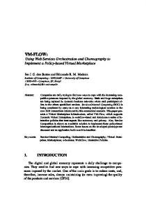
Figure 2.1 This program fragment has the following property: while looping "a + b" and "x + y" evaluate to the same value which suggests an optimization with the foUowing result:

I h:=zq-y }

I h:=a+b I

I 11 Figure 2.2 Already the basic variant (see 4.2) of our algorithm achieves this optimization. The following discussion demonstrates the effects of the five steps of our two stage algorithm. The semantic analysis of step 1.0) designates the flow graph with partitions characterizing all term equivalences wrt the Herbrand interpretation, i.e. all equivalences being valid independent of specific properties of the term operators (Figure 2.3). In particular, it detects the equivalence of "a + b" and "x + y" after the execution of either assignment.

391

L

11

(,,~,,~):=(,,,b,~+b) I

{(a,b,c):=(~,y,~+y)j [a,x Ib, y Ic, a + b,a + y,z + b,z + Yl

Figure

[a x]b, ylz,a-4-b,a+y,x+b,x-4-y ]

J

l

I

Afterwards, step 1.(ii) extends this designation for every program point to a syntactic representation of semantic equivalences which is large enough to perform our optimization:

ii ] ........ [alblcl~lylzla+bl~+y]

[alblcI=lyl~la+bl~+y]

[a,~t,~,ylc,a+b,~+y,~+b,=+y] I I [a,~lb,~lz,a+b,~+~,~+b,~+y] Figure 2.4

[

t

J

~,,

J

[

Subsequently, step 1.(iii) produces the corresponding Value Flow Graph, whose relevant part is shown in Figure 2.5:

[

[albicl=lyl

x+yl

[a,~l

Figure 2,5 The placement procedure only refers to term equivalences that are explicit in the Value Flow Graph under consideration, i.e. two terms are equivalent at a program point if they axe displayed as members of the same equivalence class in the Value Flow Graph at this point. Applying a modification of Morel/Renvoise's algorithm (step 2.0) ) to the Value Flow Graph above yields:

L

[alblclxlylzla+b~ [alblclxlwl)la+ b

L

[alblcl~x+y] x+y]

[alblel=lYlzla + i f ~ / f ~

ta, = Jb, ~¢~¢/f//z/yZ/z£/C-~.z//2/£/2A Figure 2.6

[

The inserted nodes axe the optimal computation points (the insertion of synthetic nodes is common for code motion, see Section 5). - Now, application of step 2.(ii) results in:

392

L

L

h3 := hi

b4 := h2

](a,b,c, h4):=(x,y, h3, h3) I

[(x,Y,z, h3):=(a,b, h4,h4) I

F i g u r e 2.7 Subsequent variable subsumption [Ch,CACCHM] yields the desired result (Figure 2.2).

3

Preliminaries

We consider terms t G T which are inductively built from variables v G V, constants c G C and operators op G Op. To keep our notation simple, we assume that all operators are two-ary. However, an extension to operators of an arbitrary arity is straightforward. The semantics of terms of T is induced by the Herbrand interpretation H = ( D, H0 ), where D=~, T denotes the non empty d a t a domain and H0 the function which maps every constant c E C to the datum H0(c) = c E D and every operator op E O p to the total function H0(op) : D x D--* D, which is defined by Ho(op)(tl,t2)=df(op, tl,t~) for all tl,t~ G D. ~ = { a l a : V---~D} denotes the set of all Herbrand states and ao the distinct start state which is the identity on V (this choice of a0 reflects the fact that we do not assume anything about the context of the program being optimized). The semantics of terms t G T is given by the Herbrand semantics H : T--+ (~ ~ D), which is inductively defined by: Va G ~ V t G T.

H(t)(o-) =d/

{~,(v) Ho(c) Ho(op)(H(tl)(*), H(t2)(a))

if t = v G V if t = c E C if t = op(h,t~)

As usual, we represent imperative programs as directed flow graphs G = (N, E, s, e) with node set N and edge set E. (These flow graphs are obtainable for example by the algorithm of [All] ). Nodes n E N represent parallel assignments of the form ( x l , . , z r ) : = (tl,.,tr), where r > 0 and zi = zj implies i = j , edges (n, m) G E the nondeterministic branching structure of G, and s and e denote the unique start node and end node of G which are assumed to possess no predecessors and successors, respectively. ~ r t h e r m o r e we assume that s and e represent the empty statement "skip" and that every node n G N lies on a path from s to e. The set of all such flow graphs is denoted by F G . For every node n = (x~,., zr) := (t~,., tr) of a flow graph G we define two functions 5, : T--* T

by 6 , ( t ) = q t[tl,., tdzl,., x~] for all t G T,

where tit1, .,tr/xl,., x~] stands for the simultaneous replacement of all occurrences of xi by ti in t, i E { 1 , . , r } , and 8 = : ~ - - ~ , defined by: V a G ~ V y E V . #,(a)(Y) =d! S H(ti)(a) tr(y)

if y = xi, i E {1,.,r} otherwise

6= realizes the backward substitution, and 8~ the state transformation caused by the assignment of node n. Additionally, let T(n) denote the set of all terms which occur in the assignment represented by n.

393

A finite path of G is a sequence (nl, ..,nq) of nodes suchthat (nj,nj+~) E E for j e {1, . , q - l } . P ( n l , nq) denotes the set of all finite paths from nl to nq and ";" the concatenation of two paths. Now the backward substitution functions Q : T ~ T and the state transformations 0~ : ~ --+ can be extended to cover finite paths as well. For each path p - - (m - n~,., nq - n) E P ( m , n) we define A v : T - * T by A v = a l Q ~ if q = l and A(~,.,~q_ 0 oQq otherwise, and 0 v : ~ - - ~ by Op =dr O~ if q = 1 and O(~2,.,,,q)o O~x otherwise. The set of all possible states at a node n C N is given by Now, we can define: D e f i n i t i o n 3.1 Let tl,t2 E T and n E N. Then tl and t~ are Herbrand equivalent at node n i/~ Va e S , . H ( t l ) ( a ) = H(t~)(°).

4

Construction

of a Value

Flow

Graph

The following subsections correspond to the three construction steps of a Value Flow Graph for a flow graph G, which we consider as to be given from now on.

4.1

D e t e r m i n i n g Local S e m a n t i c E q u i v a l e n c e

The semax~tic analysis determines all equivalences between program terms wrt the Herbrand interpretation (see 1.Optimality Theorem 4.6). These are expressed by means of structured partition DAGs (cp. [FKU]), which are directed, acyclic multigraphs, whose nodes are labeled with at most one operator or constant and a set of variables. Given a structured partition DAG, two terms are equivalent iff they are represented by the same node of the DAG. - T o define the notion of a structured partition DAG precisely, let ioS~,=df {TI TC(VU CU O p ) A I T ] Ew\{0}}. D e f i n i t i o n 4.1 A structured partition DAG is a triple D = (No, ED, LD), where

• (ND, ED) is a directed acyclic multigraph with node set ND and edge set ED C_ND x ND. • LD :

ND --+ ~fin is a labelling f~nction, which satisfies

1. v~ e No. IL~(~)\Vl < 1 and ~. V~,~' e No. ~ # ~ ' ~ Lo(~)nLD(~')COp • Leaves of D are the nodes 7 E ND with LD(~')AOp = ~. • An inner node 7 of D possesses exactly two successors, which we denote by 1(7) and r(7 ). •

VT,'y'C ND. LD(7)ALD(7')NOp ¢ 0 A l(7)=I(7' ) A r ( 7 ) = r ( 7 ' ) = > 7 = ' } ''.

If ND is finite, D is called a finite structured partition DAG. The set of all structured partition DAGs and the set of all finite structured partition DAGs are denoted by IP:D and iPDlln, respecHvelyo A node -? E N D program terms:

of a structured partition

DAG

is meant to represent an equivalence class of

TD(7) = ((VU C)ALD(7))u {(op, t, t') lope (OpALD(7)) A (t, t') E TD(I(')')) x TD(r("?))} Thus a full DAG represents a partition (or equivalence relation) on:

T(D) =~ U {TD(~) I~ ~ N~} C T

394

This can be illustrated as follows:

partition

DAG

[a, x lb, y la + b,a 4- y,x 4- b,z + y,z]

+,z a,x~,y

Figure 4.2 Viewing DAGs as equivalence relations makes 7~:D a complete lattice, with inclusion defined set theoretically as usual. This guarantees existence and well definedness of ~ ( P ) in:

Definition 4.3 Let D E T':D. Then 1. ~ ( D ) is the smallest structured partition DAG with Dc_7~(D) and T(Ti(D)) = T. ~. tl,t2 E T ar]e syntactically D-equivalent, iff D possesses a node 7 with ta,t2 E TD(7).

3. ta,t2 E T are semantically D-equivalent, iff they are syntactically ~(D)-equivalent. We have (cf. [St2]): T h e o r e m 4.4 Let tl,t2 E T, n E N, and We[n] E 7~2~yi~ be the structured partition DAG of the entry information at node n computed by Algorithm A.1. Then t 1 and t~ are Herbrand equivalent at node n iff they are semantically pre[n]-equivalent. Structured partition DAGs characterize the domain which is necessary to compute all term equivalences which do not depend on specific properties of the term operators. Moreover, they allow us to compute the effects of assignments essentially by updating the position of the left hand side variable:

pre-DA G

assignment

post-DAG

b:=a+b

/',,,

+,z a,

4-~z,b

a, x

,y

y

Figure 4.5 As a consequence of Theorem 4.4 we obtain:

Theorem 4.6 (1.Optimality T h e o r e m ) Given an arbitrary flow graph, Algorithm A.I terminates with a DA G-designation which ezactly characterizes all equivalences of program terms wrt the Herbrand interpretation. 4.2

Computing

the Syntactic

Representation

In the last section we constructed finite structured partition DAGs that characterize Herbrand equivalence semantically (Definition 4.3(3)). However, the placement procedure (Section 5.1) considers the pre-DAGs and post-DAGs of a designation of a flow graph as purely syntactical objects, i.e. terms are considered equivalent iff they are syntactically equivalent (Definition 4.3(2)). Of course, it is not possible to finitely represent all Herbrand equivalences syntactically. However, it is possible to represent finite subsets that are sufficient for obtaining our optimality results (see Section 5.3). This is done by computing for every node n of G a finite set of terms T~, f that is

395

sufficient to represent all necessary equivalences at n syntactically, i.e. as the restriction of 7-/(D) to T,~I. Here, we sketch two strategies for the construction of such term closures. The first strategy associates every node n with the set of terms representing values that must be computed on every continuation of paths from s to n that end in e, and the second strategy with the set of terms representing values that may be computed on a continuation of a path from s to n ending in e. Both term closures are computed by backward analysis. The first strategy algorithm iteratively computes approximations of the closure for a node as the meet over the current approximations of the closures of its successors. The second strategy algorithm is essentially dual. However, it is necessary, to constrain the iteration here because the straightforward dual algorithm would not terminate. These two strategies define the basic and full variant of our two stage algorithm. There is another important variant of our algorithm, which we call RWZ-variant. It is based on a strategy for computing closures, which starts by invoking the first strategy algorithm. Subsequently, it applies this algorithm to all flow graphs that result from considering nodes as end nodes whic]5 possess at least one "brother".

4.3

The Value Flow Graph

A Value Flow Graph connects the term equivalence classes of a DAG designation according to the data flow. Essentially, its nodes are the equivalence classes and its edges representations of the data flow. For technical reasons we define the nodes of a Value Flow Graph as pairs of equivalence classes. However, identifying these pairs with their second component leads back to the original intuition, which will be referred to in the next section. In the following let us assume that every node n of G is designated by a pre-DAG pre(n) and a post-DAG p o s t ( n ) according to the remits of Section 4.2. For the sake of readabifity we abbreviate 0 (Npre(,) x Npost(,)) by I" and define a subset 8 _ C I" (in the following 7~ 6 7' nfiN

stands for (% 7') 6 ~ - ) by: V(7,7') 6 F. 7' ~ 7' 4~)'4t 3n 6 N. Tpre(n}(7)_D&(Tpost(n}(7')). Let now ® denote a new symbol, and preda and suceG functions that map a node of G to its set of predecessors and successors, respectively. Then the technical definition of the Value Flow Graph for the DAG designation under consideration is as follows: Definition 4.7 A Value Flow Graph V F G is a pair (VFN, VFE) eonsistin 9 of

• a set of nodes V F N C_ . ON( (Npre(,}U {{D}) x (Npost{.}U {(D} ) ), where 6

71~---72 6 /~78.71~--7s if 71 # ®A~2= ® 6 if ~ = ® ^ ~ 2 # ®

v=(71,72) 6 V F N ¢ = ~

• a set of edges V F E C_V F N x VFN, where

(v,u') 6 V F E ¢=~#

{

v'h#®Au$2#0 A ~;(~') e su~a(X(~)) ^ Tpre{~{v,}}(v'h)_CTpost{~{u}}(u$2)

where ".h" and "~.2" denote the projection of a node v to its first and second component respectively, and A/'(u) the node of the flow graph ~,hat is related to v.

396

Thus, nodes v of the Value Flow Graph are pairs (71,72), where 71 is a node of the pre-DAG and 72 a node of the post-DAG of a node n of G, such that 71 and 72 represent the same values, i.e. satisfy the inclusion Tpre(n)(71)D{t ] 3t' e Tpost(n)(72 ). t = ~,(t')}. Edges of the Value Flow Graph are pairs (v,v'), such that A/'(v) is a predecessor of A/'(v') and values are maintained along the connecting edge, i.e. Tpre(./V'(v,))(V'~l)GTpost(.h~(v))(v~2). Finally, given a Value Flow Graph V F G , we define:

VFNs=41 { u 1N(predvFG(V) ) # preda(N(u) ) V A/'(v) = s} and

VFN e =af { u IN(8ttCCVFG(Y) ) # 8uccG( 4~ (1/) ) V .~ ( v ) -~ e} where predVFG and succvFG denote functions that map a node of V F G to its set of predecessors and successors, respectively.

5

Optimal Placement of Computations

The placement procedure is optimal in its own right. It works for any Value Flow Graph, which need not be produced by the first stage algorithm or restricted to Herbrand equivalence. Before going into details, let us mention a technicality, which is typical for code motion (cf. [I~WZ]). Edges, leading from a node with more than one successor to a node with more than one predecessor, are split by insertion of a synthetic node. This is necessary in order to avoid "deadlock" during the code motion process, which may arise as illustrated in Figure 5.1(a). There the computation of "a + b" at node 3 is partially redundant wrt to the computation of "a + b" at node 1. However, this partial redundancy cannot safely be eliminated by moving the computation of "a + b" to node 2, because this may introduce a new computation on a path which leaves node 2 on the right branch. On the other hand, it can safely be eliminated by moving the computation of "a + b" to the synthetic node 4 as it is displayed in Figure 5.1(b).

11

I

21/ ......... I

11 h:=a L

o+b l F i g u r e 5.1

2i/ h

\

I

I

~

The following consideration assumes this simple transformation. In fact, the corresponding transformation of the Value Flow Graph is trivial as well, because all the inserted nodes represent skip-statements.

5.1

D e t e r m i n a t i o n of the C o m p u t a t i o n Points

The point of the placement procedure for computations is the solution of the following Boolean equation system (see Equation System 5.2), which we modified to work on Value Flow Graphs rather than flow graphs directly, in order to capture semantic equivalence. FoUowing [MR], the names of the predicates are acronyms for the properties "local auticipabili~y", "availability" and

"placemen~ possible":

397

E q u a t i o n S y s t e m 5.2 (Boolean E q u a t i o n S y s t e m ) • The Frame Conditions (Local Properties): A N T L O C ( v ) ¢=~ vhn

T(tC(v)) # 0

AVIN(v) = P P I N ( v ) = f a l s e if v E VFNs P P O U T ( v ) =false if v

E

VFNe

• The Fixed Point Equations (Global Properties): AVlN(v) AVOOT(v) PPIN(v)

PPOUT(v)

¢=*

I] AVOUT(v') v' e pr,d(v)

~

AVIN(v) V P P O U T ( v )

¢=~

AVlN(v) A ( A N T L O C ( v ) V P P O U T ( v ) )

¢==>

II

~

PPIN(#)

Algorithm A.2 computes the greatest solution of this system, which determines the computation points by means of I N S E R T ( v ) = # P P O U T ( v ) A -~PPIN(v)

5.2

Placing the Computations

The placement Algorithm A.3 proceeds in three steps: 1. It marks all nodes of the Value Flow Graph that occur on paths that lead from nodes satisfying I N S E R T to nodes satisfying A N T L O C . 2. It associates with every marked node of the Value Flow Graph an auxiliary variable. This is a new auxiliary variable, if the marked node either satisfies I N S E R T or has more than one predecessor in the Value Flow Graph. Otherwise the auxiliary variable of its unique predecessor in the Value Flow Graph is taken. 3. It initializes at every node of the Value Flow Graph satisfying I N S E R T its associated auxiliary variable by its initialization term. (Initialization terms of a node v of the Value Flow Graph are minimal representatives of its corresponding equivalence class v.L2.) If two marked nodes which are associated with different auxiliary variables, say h~ and hi, are connected by an edge in the Value Flow Graph, a trivial assignment hi := hk is added at the end of the first node. Finally, original computations of the flow graph are replaced by the corresponding auxiliary varial)les. Note, in order to eliminate all redundancies at once, the initializations of auxiliary variables are split into sequences of assignments that only have a single operator in their right hand side expression.

398

5.3

Optimality

Results

An analysis of the Boolean Equation System 5.2 delivers not only the correctness of the derived program transformation, but also its optimality. Intuitively, a flow graph is defined to be optimal wrt a Value Flow Graph if it is "best" in the class of branching structure preserving flow graphs that are "safe" and "complete" for it. Here "best" means that it possesses a minimal number of computations on every path, and "safe" ("complete") that it computes on every path at most (at least) as many values. A formal definition of this notion of optimality is complicated, because all these properties need to be defined in terms of the Value Flow Graph. We will therefore only sketch the formal treatment. For this purpose we will assume (without loss of generality) that the synthetic nodes are already inserted, that linear sequences of nodes are abbreviated by a single node (basic block), and that the Value Flow Graph covers all computations of the underlying flow graph, i.e.: V n e N VteT(n) 3~EVFN. Af(v)=r~ A tETpre(,)(v~t) Now, let V F G be a Value Flow Graph for a flow graph G = (N, E, s, e), and G' = (N', E', s', e') a branching structure preserving flow graph for G, i.e. there exists a graph isomorphism k~ from G' onto G with V(s') = s and k~(e') = e. Furthermore assume that p e P(s, e) and p' = (nl, .., nq) e P(s', e') with q~(p') = p, and let VFG(p) denote the graph that results from uurolfing V F G along the path p. Then V F G ( p ) is a collection of trees, which we will refer to as the VFG-values of p. This notion is motivated by the fact that VFG(p) defines an equivalence relation on (potential) term occurrences wrt p whose equivalence classes contain computations that evaluate to the same value during the execution of p, and that these classes are maximal such wrt V F G . Given a V F G value C of p, rgv(C)-=aI {nl 13v E VFNe. Af(t,) = nl} denotes the range of C. A computation t' of p' at node nl is q!-covered by a VFG-value C of p if ~(ni) e rgv(C ) and if t' is covered by C at k~(ni), or if Q,_t(t') is kg-covered by C at ni-1. This complicated definition is necessary because a computation in p' need not match a term in V F G , for example because of additional (auxiliary) variables in G'. CwG(p) denotes the set of all VFG-values of p that cover at least one computation of p, and Cw¢(~,p') the maximal set T, or the smallest set of VFG-values of p which ~-cover all computations of p', if such a set exists. After this preparation we are able to define the central notions of our optimality concept. G' is VFG-safefor G if CVFG(ffJ,p') C_ Cvm(ffd(p')), andit is VFG-complete for G if Cvm(q2,p') D Cvm (q2(p')) for all p' e P(s', e'). Moreover, p' is better than p if it contains at most as many (non trivial) computations as p, and G' is better than G if p' is better than q~(p') for all p t e P(s', e'). Finally, G is VFG-optimal if it is better than any branching structure preserving G' that is VFG-safe and VFG-complete for G. T h e o r e m 5.3 ( 2 . O p t i m a l i t y T h e o r e m )

Every flow graph transformed by the second s~age of our algorithm is VFG-optimaI. Let us now consider the combined effect of the two stages of our algorithm. As mentioned already, it is not possible to finitely represent all Herbrand equivalences syntactically. However, using the 1.Optimality Theorem 4.6 we can show that there exists an infinite Value Flow Graph V F G o ¢ that even represents all global Herbrand equivalences. This Value Flow Graph is the natural extension of a given Value Flow Graph where all partition DAGs D are replaced by 7/(D), see Definition 4.3.

Definition 5.4 A VFGc,~-optimal program is called Herbrand optimal. We have: T h e o r e m 5.5 ( H e r b r a n d O p t i m a l i t y )

Every flow graph transformed by our two stage algorithm in the full variant is Herbrand optimal.

399

Herbrand optimal transformations may cause unboundedly many reinitializations of auxiliary variables in order to eliminate a single redundant computation. Thus, the costs of these reinitializations can easily exceed the costs of the eliminated computation. Motivated by this problem Rosen, Wegman and Zadeck introduced a notion of optimality, which is based on an additional technical constraint (see [RWZ] for details). Referring to this notion as RWZ-optimallty we can prove: T h e o r e m 5.6

(RWZ-Optimality)

Every flow graph transformed by our two stage algorithm in the RWZ-variant ~ RWZ-optimal. As usual for code motion, our algorithm is devoted to the costs of computations. However, costs for register loading and storing are subsequently taken care of by variable subsumption. An algorithm based on the graph coloring techniques of [Ch,CACCHlVl] is implemented for this purpose. Finally, let Trans : F G --* F G be the operator specified by the full variant of our algorithm. Then we obtain by means of the 2.Optimality Theorem 5.3: C o r o l l a r y 5.7 Trans i8 idempotent, i.e. VG e FG. Trans(G) = Trans(Trans(G)). In particular, the full variant of our algorithm covers all second order effects (cf. [RWZ]).

6

Complexity

The second stage of our algorithm can be applied to arbitrary Value Flow Graphs, yielding optimal results relative to the equivalence information represented (see 2.Optimality Theorem 5.3). We therefore estimate the worst case time complexity, which as usual is based on the assumption of constant branching and constant term depth, independently for both stages. This requires the following t:hree parameters: the number of nodes of a flow graph n, the complexity of computing the meet of two equivalence informations m, and the maximal number of Value Flow Graph nodes which are associated with a single node of the underlying flow graph, p. This yields for the complexity of the five steps of our algorithm: 1. Construction of a Value Flow Graph for the Herbrand interpretation:

(i)

Determination of semantic equivalences: O(n2.m). Here "n 2" reflects the maximal length of a descending chain of annotations of a flow graph. In fact, the number of analysis steps of Algorithm A.1 is linear in this chain length. This can be achieved by adding those nodes to a workset whose annotations have been changed. Then processing a worklist entry consists of updating the annotations of all its successors. This can be done in O(m) because of our assumption of constant branching. To our knowledge, the exact nature of m is not studied in previous papers. This is probably due to the fact that, in practice, this effort hardly increases linearily in the size of the analysed program, and therefore is regarded as harmless. However, DAGs that arise during the analysis may represent sets of terms which increase exponentially in n. Inspire of this fact, we conjecture that the compact representation of these sets by means of structured partition DAGs, together with the constraint that the DAGs arise during the analysis of a particular program, allows us to show that the number of nodes in such a DAG only increases quadratically in n. This conjecture would suffice to prove an overall complexity of O(n 4) for the first step, because we know that the meet of two DAGs can be computed essentially linearily in the size of the resulting DAG.

400

(ii) Computation of the syntactic representation of the semantic equivalences: This complexity depends on the variant chosen. Whereas the basic variant and the RWZ-variant are both O(n3), the full variant seems to be exponential in n. (iii) Construction of the Value Flow Graph: O(n*#). This is based on two facts. First, if there exists an edge in the Value Flow Graph between two nodes vl and v2 then the corresponding nodes A]'(vl) and AZ(v2) of the flow graph are connected as well. Thus every edge of the Value Flow Graph is associated with an edge of the original flow graph. Second, the effort to construct all edges of the Value Flow Graph that correspond to a single edge (n, m) in the original flow graph is linear in the number of Value Flow Graph nodes that annotate n, which can be estimated by ~u. 2. Optimal placement of the computations: (i) Determination of the computation points: O(n*/~). The argument needed here is based on that of the first step, however, we do not have constant branching, and the algorithm here is bidirectional. This leads to the product n*# because all nodes of the Value Flow Graph can be updated once by executing only two elementary operations per edge of the Value Flow Graph, and the number of edges in a Value Flow Graph can be estimated by O(n*#). (it) Placing the computations: O(n*#). This is straightforward. Let us finally give an estimation of the worst case time complexity of the practically motivated RWZ-variant. Here, O(/~) can be approximated by O(n2). In fact, exploiting the specific nature of the RWZ-closure already during the first step, we arrive at an algorithm with an overall complexity of O(n4). Assuming our conjecture, this result is also true for the RWZ-vadant of our two stage algorithm presented above.

?

Conclusion

We have shown, how to combine semantic algorithms with syntactic ones, in order to obtain maximal optimization results. This technique, which is based on the introduction of Value Flow Graphs, has been illustrated by developing a two stage algorithm for the optimal placement of computations within a program. In addition to their optimality, algorithms developed by means of this technique are easily to extend, because the separation of their semantic part from their (independently optimal) syntactic transformation part makes them modular. This modularity allows to independently enhance the semantic properties by modifying the first stage, and the transformation capacity by strenghtening the second stage. In our current implementation, the first stage is extended to deal with cor~tant propagation and constant folding (see [SK1,SK2]). An extension of the second stage to strength reduction ([ACK,CK,JD1,JD2 D is under development.

Acknowledgements The presentation in this paper profited from discussions with Torben Hagerup, Mark Jerrum, Barry Rosen and Ken Zadeck.

401

References [All]

F.E. Alien. "Control Flow Analysis". ACM Sigplan Notices, July 1970

[ACK] F.E. Allen, J. Cocke and K. Kennedy. "Reduction of Operator Strength". In: St. S. Muchnick and N. D. Jones, editors. "Program Flow Analysis: Theory and Applications", Prentice Hall, Inc., Englewood Cliffs, New Jersey 07632, 1981 [Ch]

G . J . Chaitin. "Register Allocation and Spilling via Graph Coloring". IBM T. J. Watson Research Center, Computer Science Department, P.O. Box 218, Yorktown Height, N. Y. 10598, 1981

[CACCHM] G. J. Chaitin, M. A. Auslander, A. K. Chandra, J. Cocke, M. E. Hopkins and P. W. Markstein. "Register Allocation via Coloring". IBM T. J. Watson Research Center, Computer Science Department, P.O. Box 218, Yorktown Height, N. Y. 10598, 1980 [CK]

J. Cocke and K. Kennedy. "An Algorithm for Reduction of Operator Strength". Communications of the ACM, 20(11):850-856, 1977

[FKU] A Fong, J. B. Kava and J. D. Ullman. "Application of Lattice Algebra to Loop Optimization'. 2~a POPL, Polo Alto, California, 1 - 9, 1975 [JD1] S.M. Joshi and D. M. Dhamdhere. ".4 Composite Hoisting-Strength Reduction Transformation for Global Program Optimization - Part I n. Internat. J. Computer Math. 11, 21 41, 1982 [JD2] S.M. Joshi and D. M. Dhamdhere. ".4 Composite Hoisting-Strength Reduction Transformation for Global Program Optimization - Part II'. Internat. J. Computer Math. tl, 111 126, 1982 -

[Kil]

G.A. Kildall. "Global Expression Optimization during Compilation". Technical Report No. 72-06-02~ University of Washington, Computer Science Group, Seattle, "yVashington, 1972

[Ki2]

G.A. Kildall. ".4 Unified Approach to Global Program Optimization". 1.t POPL, Boston, Massachusetts, 194 - 206, 1973

[MR]

E. Morel and C. Renvoise. "Global Optimization by Suppression of Partial Redundancies". Communications of the ACM, 22(2):96-103, 1979

[RWZ] B. K. Rosen, M. N. Wegman and F. K. Zadeck. "Global Value Numbers and Redundant Computations'. 15~h POPL, San Diego, California, 12 - 27, 1988 [St1]

B. Steffen. "Optimal Run Time Optimization. Proved by a New Look at Abstract Interpretations". TAPSOFT'87, Pisa, Italy, LNCS 249, 52 - 68, 1987

[St2]

B. Steffen. "Abstrakte Interpretationen beim Optimieren yon Programmlaufzeiten. Ein ()ptimalitgtskonzep~ und seine Anwendung". PhD thesis, Christian-Albrechts-Universit£t Kiel, 1987

[SK1]

B. Steffen and J. Knoop. "Finite Constants: Characterizations of a New Decidable Set of Constants". 14~h MFCS, Por~bka-Kozubnik, Poland, LNCS 379, 481 - 491, 1989

[SK2]

B. Steffen and J. Knoop. "Finite Constants: Characterizahons of a New Decidable Set of Constants'. Extended version of [SK1], LFCS Report Series, ECS-LFCS-89-79, Laboratory for Foundations of Computer Science, University of Edinburgh, 1989

402

A

Appendix:

The

Algorithms

Algorithm A.1 (The Semantic Analysis of Step 1.(i)) Input: An arbitrary flow graph G = (N, E, s, e)with unique start node s and unique stop node e, which are assumed to possess no predecessors and no successors, respectively. Output: A designation of G with pre-DA Gs (stored in pre) and post-DA Gs (stored in post), characterizing valid and complete equivalence information at the entrance and at the exit of every node n • N, respectively.

Remark: _1. denotes the "empty" data flow information and T its complement, the "universal" data flow information, which is assumed to "contain" every data flow information. [ ] denotes the local analysis component and [q the meet operation. ([ ] and [1 operate on DAG-structures). pred(n)=d! {m I(m,n) e E} and succ(n)=df {m I(n,m) • E} denote the set of all predecessors and successors of a node n, respectively. The variable workset controls the iterative process, and the auxiliary variable meet stores the result of the most recent meet operation. (Initialization of the designation arrays pre and post and the variable workset) F O R all nodes n • N DO IF n = s T H E N (pre[n], post In]):= (±, [ n 2(1)) ELSE (pre[n],post[n]):= (-1-,T) FI OD; workset := {s}; ( Iterativc fixed point computation) W H I L E workset ~ ~) DO LET n • workset BEGIN workset := workset\ {n } ; (Update the "environment" of node n ) F O R all nodes m • succ(n) DO

meet := pre[m] n post[n]; IF pre [m] -1 meet THEN pre[m] := meet; post [m]:= i m ](pre [m]); workset := worksetU {m} FI OD END OD. Algorithm A.2 (Solution of the Boolean Equation System (Step 2(i))) Input: A Boolean equation system which is completely initialized wrt the local property ANTLOC. Output: The greatest solution of the Boolean equation system.

Remark: With every node of the Value Flow Graph the predicates ANTLOC, AVIN, AVOUT, PPINand P P O U T are associated. However, only ihe later four are involved in the fixed point iteration, which therefore operates on the fourfold cartesian product of the complete semi-lattice {false, true} with false r- true. pred(u)=df {#] (#, u) fi gEE} and succ(v)=~ {# [(u, I~) • gEE} denote the set of all predecessors and successors of a node u, respectively. The variable workset

403 controls the iterative process. For notational convenience we abbreviate (AVIN(u), AVOUT(v), PPIN(u), P P O U T ( u ) ) by fu. The auxiliary variable f store8 the result of the most reeen~ application of the local analysis component, and avin and ppout are further auxiliary variables. (Initialization) F O R all nodes u E VFN D O flu := (true, true, true, true) OD; F O R all nodes u e VFNs D O (AVIN(u), P P I N ( v ) ) : = (falze, fulse) OD; F O R all nodes u E VFNe D O P P O U T ( u ) := false OD; workset := VFNsU VFNe; ( Iterative fixed point computation) W H I L E workset ¢ 0 D O L E T v E workset BEGIN workset := workset \ {u}; (Update the Uenvironment" of node u ) F O R all nodes # e pred(v)Usucc(u) D O I F # e pred(v) THEN ppout := P P O U T ( # ) A E{PPIN(A) I A e succ(#) A Af(~) = Af(u)}; /~:= (AVIN(#), AVIN(#) Y ppout, AVIN(#) A ( A N T L O C ( # ) Y ppout), ppout ) ELSE avin := AVIN(#) ^ AVOUT(u); f : = (avin, av/nVPPOUT(#), avinA(ANTLOC(p)VPPOUT(,u)), P P O U T ( # ) ) FI; IF ~-Tf THEN

f.:=~ workset := workset U {#} FI OD

E~ OD.

Algorithm A.3 (The Optimizing Program Transformation (Step 2(ii))) I N P U T : A flow graph G and an accoeiated Value Flow Graph V F G with attached predicate designation characterizing the greatest solution of the Boolean Equation System 5.~. O U T P U T : The transformed flow graph GT. In GT auxiliary variables are initialized at the optimal computation points by their minimal computation form, wrt to the equivalence information expressed by V F G . Original computations are replaced by auxiliary variables. R E M A R K : The algorithm consists of three phases, namely

• Marking of the definition.use chains in VFG. • Allocating of the auxiliary variable numbers. • Transforming of the flow graph, namely - Initializing auxiliary variables at their computation points by their computation forms. - Introducing spill code for the generated auxiliary variables. -

Substituting original computations by a reference to their covering auxiliary variable.

404

The marking of a node u G VFN is indicated by the predicate mark(u), the number of an associated auxiliary variable is denoted by nr(u) and the variable count indicates the number of the last generated auxiliary variable. (Phase 1: Marking of the definition-use chains in V F G ) F O R all nodes u G VFN D O mark(v) := false O D ; zoorkset := { u e VFN I A N T L O C ( u ) } ; W H I L E workset ¢ ~ D O L E T u G workset BEGIN workset := workset \ { u } ; mark(u) := true; I F - , I N S E R T ( y ) T H E N wor~et := work~ct U {u' G pred(u) 1-~ mark(u') } F I END OD;

( Phase 2: Allocating auxiliary variable numbers) count := O; F O R all nodes u G VFN D O nr(u) := 0 0 D ; workset := {u e VFN II N S E R T ( u ) } ; W H I L E workset ~ 0 D O L E T u G workset BEGIN

~oor/~et : = ~,orkset mark(v) := f~l~e;

\{u};

I F I N S E R T ( v ) V Ipred(u) I > 2 THEN

count := count + 1;

nr(u) := count ELSE (assume pred(u) = {u'}) nr(u) := ~r(u') FI;

~,or~,et := ~,or~et u {u' e sure(u) I mark(u) } END OD;

( Phase 3: Transformation of the flow graph) ( Initializing auxiliary variables at their computation poin~ by their computation forrn~) F O R all nodes n G N D O wor~et := {u e VFN I I N S E R T ( u ) ^ N ( v ) = n }; W H I L E wor~et ~ O D O L E T u E {u' E worluet [VP 6 worl~et . ~ ~ succ*(u'~2)} BEGIN

~or~et := wor~et \{u}; IF npost(n)(Ui2)n(VU C) # 0 THEN L E T z E Lpost(n)(U$2)n (VU C) BEGIN

Attach the assignment hnr(u):= x] at the end of node n END

405

ELSE L E T op E Lpost(n)(V~2),.. v' e VFN. v'~2=l(vl2), P E VFN. V~2=r(VI2) BEGIN a**ach ~he a.ignment [ h . . , ) : = h..,,)o~,h..(~,) ] at ~he end of node n END FI

END OD OD; ( Introduc~ing spill code for the generated auxiliary variables) F O R all nodes v, u' e {~ e YFglnr(P) # 0} DO IF ~ e pred(~') ^ nr(~) # ~r(~') THEN a~a~h a eo~ponen~ of spill ~ode [(.., h,,,,), ..) := (.., h,~C~,),..)] a~ ~he en,~ of,~ode FI OD; ( Substituting original computationz by a reference to their covering auxiliary variable) F O R all nodes n G N DO workaet := {v e V F N I A N T L O C ( v ) AAf(v) =n}; W H I L E worh~et • $ DO LET ve {v'e workset IVp e worI~et. P+I ~ pred*(v'~a)} BEGIN workaet := workaet \{V}; Replace all original computation, t • T(n)N Tpre(n)(V.~,) by h.,w) END OD OD.

.~'(~,)