The visualization of turbulence data using a ... - Wiley Online Library
Recommend Documents
Feb 5, 2015 - Proteomics 2015, 15, 1375â1389. 1375. DOI 10.1002/pmic. ... Accepted: February 9, 2015 ..... munity best practices in terms of scientific software develop- ment and R .... Figure 5. Illustration of the MALDIquant preprocessing pipelin
Received 26 August 2011; revised 4 November 2011; accepted 7 November 2011; published 5 January 2012. ... wind speed with that of a cup anemometer for wind energy ..... [12] The measurements were performed at the Danish. National ...
Dec 19, 2015 - L. Kaser1, T. Karl2, B. Yuan3,4, R. L. Mauldin III5,6, C. A. Cantrell5, A. B. Guenther7, E. G. Patton1,. A. J. Weinheimer1, C. Knote1,8, J. Orlando1 ...
Aug 15, 2012 - improved data visualization approaches are proposed as ... Keywords: data visualization technique; structural index; empirical phase diagram; ...
present an optimized rendering algorithm for hybrid volume-geometry data based on the ... efficient visualization of hybrid data sets as they occur in today's.
combined data set contained 187,404 records with injury diagnoses from approximately 616,000 ED patient visits, represen
Sep 4, 2015 - Monash University, Melbourne, Victoria, Australia, 5Department of Geophysics, ... College of Marine Science, University of South Florida, St.
May 22, 2012 - Citation: Kilcher, L. F., J. D. Nash, and J. N. Moum (2012), The role of turbulence stress divergence in decelerating a river plume, J. Geophys.
Modeling Migration Careers, Using Data from a. British Survey. Development of more sophisticated techniques for modeling longitudinal data has implications ...
ABSTRACT: In the analysis of water quality data, samples with concentrations ... analyze Type I censored data for biomedical applica- tions, but few have been ...
Benjamin H. Letcher*. U.S. Geological Survey, Leetown Science Center, S.O. Conte Anadromous Fish Research Center,. 1 Migratory Way, Turners Falls, MA ...
Jul 4, 2014 - and Gundagai (600532E 6119073N) and Howlong (467090E. 6017897N) in the east and west, respectively (a distance of. ~120 km) (see ...
Jun 14, 2011 - A com- monly used filter is the Gaussian filter (ISO 11562,. '96). It has a ... library.com) ..... Jiang X, Scott PJ, Whitehouse DJ, Blunt L. 2007a.
Abstract: The development of a maintenance program .... only in limited areas of application. However .... is implemented through the application of coefficient,.
(Right panel) Visualization of the rDNA region with GFP-lacI fusion protein. The fluorescence ..... from Discosoma sp. red fluorescent protein. Nat. Biotechnol.
Jun 29, 2010 - 2Rural Economic Development Programme, Teagasc, Athenry, Co., .... The key motivating reason for using MLM is to make a formal distinction between ..... admission (binary data) and the number of nights patients spent in ...
Woudenberg, S.W., Conkling, B.L., O'Connell, B.M., LaPoint, E.B.,. Turner, J.A. & Waddell, K.L. (2010). The forest inventory and analysis database: database ...
spectral power at the StilesâBurch primary wavelengths. Graphs and power ratios are used to compare the defini- tions for two alternative matches to the same ...
Jun 2, 2016 - EFFECTS OF LABOR REALLOCATION: A PANEL DATA ANALYSIS. DIMITRIOS ..... data, estimate the dynamic effects of regional employment.
data rescue and processing activities have been pro- hibitive, and in those cases where it has been possi- ble, the raw data has had to have been converted to.
a rapid increase in the velocity or speed of data creation. ⢠an extension in the variety of data types available. Therefore Big Data is not just lots and lots of ...
Four-dimensional (4D) sonography with spatiotemporal image ... Gynecology, Leiden University Medical Center, ... prenatal diagnosis; pulmonary valve; spatiotemporal image correlation .... version 9.2 program (SAS Institute Inc, Cary, NC) .... BPD ind
spatiotemporal image correlation (STIC) ... Ulsan College of Medicine, Asan Medical Center, South Korea. Objective: We ... suppmat/index.html. OC33.06.
[1] The problem of turbulence is ubiquitous in the Earth sciences, astrophysics and elsewhere. Virtually the only theoretical paradigm that has been seriously ...
The visualization of turbulence data using a ... - Wiley Online Library
Jul 10, 2006 - The visualization of turbulence data using a wavelet- based method. C. J. Keylock*. Earth and Biosphere Institute and School of Geography, ...
Earth Surface Processes and Landforms Visualization of turbulence Earth Surf. Process. Landformsdata 32, 637–647 (2007) Published online 5 September 2006 in Wiley InterScience (www.interscience.wiley.com) DOI: 10.1002/esp.1423
637
Technical communications
The visualization of turbulence data using a waveletbased method C. J. Keylock* Earth and Biosphere Institute and School of Geography, University of Leeds, UK
*Correspondence to: C. J. Keylock, Earth and Biosphere Institute and School of Geography, University of Leeds, Woodhouse Lane, Leeds LS2 9JT, UK. E-mail: [email protected] Received 17 March 2006; Revised 26 June 2006; Accepted 10 July 2006
Introduction An analysis of coherent structures within a turbulent flow requires the application of appropriate algorithms for the identification of particular flow events as well as the calculation of flow properties such as the turbulent stresses and vorticity. In geomorphological studies this may well then involve linking sediment transport events to the instantaneous flow structure (Heathershaw and Thorne, 1985; Nelson et al., 1995). In fluvial and oceanographic research, recent advances in technology mean that it is now possible to go into the field and obtain high frequency information for three orthogonal velocity components at a point using an acoustic Doppler velocimeter (Kraus et al., 1994; Lane et al., 1998) or at a variety of depths using acoustic Doppler current profilers (Simpson et al., 1996; Kostaschuk et al., 2005; Parsons et al., 2005). In addition, the increasing use of sophisticated techniques such as large-eddy simulation (Lesieur and Métais, 1996; Keylock et al., 2005) permits explicit analyses of aspects of turbulence structure from numerical modelling output. The simplest way to highlight important flow events is to undertake a Reynolds decomposition of the velocity timeseries to obtain the fluctuating velocity signal: u′i = ui − ui
Table I. Definition of flow quadrants in terms of downstream (u = ux = u1) and vertical (w = uw = u3) velocity components.
Quadrant name Outward interaction Ejection Inward interaction Sweep
Quadrant number
Sign of u1′
Sign of u3′
Contribution to Reynolds stress
1 2 3 4
+ − − +
+ + − −
Negative Positive Negative Positive
with ux in order to maintain a positive Reynolds stress (Hudgins and Kaspersen, 1999). A recent example of the use of this method is due to Roy et al. (2004), who developed their low and high speed wedge model for flow in gravel-bed rivers using this detector. However, studying two components gives improved results (Lu and Willmarth, 1973; Bogard and Tiederman, 1986) and is the most commonly used approach in the hydraulic (Biron et al., 1996; Ferguson et al., 1996) and atmospheric sciences (Katul et al., 1994). Based on the joint behaviour of the two components, one may define quadrant flow events as explained in Table I. Because Reynolds stresses are given by
τ ij = − ρui′u ′j
(2)
it follows that in a boundary-layer flow τij is dominated by the action of ejection and sweep events that make positive contributions to the shear stress with, typically, ejections correlated with entrainment of material into suspension (Cellino and Lemmin, 2004) and sweeps leading to the movement of bedload. However, as noted by Nelson et al. (1995), sweeps are not necessarily more effective than outward interactions at mobilizing bedload; it is just that events of the requisite size are more frequent. A deeper understanding of the behaviour of different quadrants in a shear flow was provided by Nakagawa and Nezu (1977), who gave results for the proportion of time occupied by and shear stress exerted by an open channel flow in each of the four quadrants by deriving the conditional probability density functions for each quadrant from a third-order Gram–Charlier distribution. Analysis of all three velocity components using an octant based approach (Table II) is less common but examples do exist in the literature. For example, Olçmen et al. (2006) use octants to study an extended version of a turbulence model proposed by Nagano and Tagawa (1990). While the transverse component is less significant in terms of boundary-layer theory, knowledge of its relation to the other velocity components may be important for eddy-structure analysis, validating large-eddy simulations or in the application of more sophisticated model validation criteria (Moeckel and Murray, 1997; Keylock, in press). Hence, whether one is analysing a signal consisting of one, two or three velocity components, there will often be a desire to visualize the data in a simple and effective manner. This aim of this technical communication is to introduce some computer routines that assist such visualization. I describe the underlying principle behind these algorithms and illustrate the type of output that is obtained below. The approach taken is to use a wavelet transform to decompose the velocity field so that intensive quantities can be identified by eye and correlated to particular flow events.
Table II. Definition of octants introduced in this paper. The sign of the lateral (v = uy = u2) velocity component is added to the quadrant number. Octant number −1 +1 −2 +2 −3 +3 −4 +4
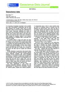
Figure 1. A u-level decomposition of a time-series for thresholds of 0·5 σ1, 1·0 σ1 and 1·5 σ1. The normalized fluctuating velocity is shown in (d) as a solid black line, with dotted lines indicating the thresholds. The panels above give the events exceeding the three different thresholds with positive exceedances given in black and negative in white, and data that fall into the ‘hole’ are given in grey.
Signal Thresholding and Visualization Figure 1 shows an example normalized signal in the bottom panel together with six horizontal lines indicating the three chosen thresholds at both positive and negative positions. The number of exceedances clearly decreases as the threshold increases. Buffin-Bélanger et al. (2000) presented a method for visualizing the space–time correlation structure of simultaneous measurements made at various heights in a gravel-bed river. The approach taken here is inspired by the type of output that their work produced, but applies to time-series data from a single location, indicating different thresholds on the same plot rather than different heights. The method could be generalized to incorporate information gained from more than one sensor by converting the plots from two to three dimensions. An inspection of Figure 1 clearly shows that the exceedance of H = 1·5 at t = 30 is a different type of event to that at t = 82. The former arises due to relatively small high frequency fluctuations superimposed on a large, low frequency positive departure from the mean. The latter is a sudden and dramatic excursion from the mean that is not superimposed on an obvious larger scale fluctuation. It would be desirable to visualize this information in a clear manner so that the scales of turbulence that actively contribute to an event can be determined, which may in turn be linked to different scales of processes. The method chosen to accomplish this uses wavelet analysis to decompose the signal into different frequencies while retaining information in the time domain.
Visualizing the Active Scales of Turbulence Interest in using wavelet analysis in environmental turbulence studies has grown since the earliest applications (Farge, 1992; Hagelberg and Gamage, 1994; Smith et al., 1998). The method is a multiresolution method for analysing data based on translation and dilation of a compactly supported (i.e. finite length) function called a mother wavelet along a signal and the convolution of this function with the signal. It permits time and frequency information to be seen at the same time, a deficiency of spectral methods that only provide frequency information. The continuous wavelet transform (CWT) for a signal g that varies with time t based on a mother wavelet ψ is given by
Figure 2. A wavelet decomposition of a time-series showing the results for a u-level threshold of 1·5 σ1. The normalized fluctuating velocity is shown in (c) as a solid line with the locations exceeding the threshold given by vertical dotted lines. The wavelet coefficients shown in the remaining panels are normalized by the global wavelet variance (a) and the scale-by-scale wavelet variance (b) with darker values indicating a higher value for the coefficients. Coefficients that are opposite in sign to the detected fluctuation are set to zero here.
Figure 3. A wavelet decomposition of a time-series showing the results for a u-level threshold of 1·0 σ1. See Figure 2 for additional information.
Figure 4. Wavelet coefficients resulting from an SWT decomposition of the time-series shown in the previous figures. The magnitude of the coefficients is shown with higher values shown in black (in accord with Figures 2 and 3).
accounted for and it can be seen that the high frequency coefficients that generated the ninth exceedance were, on their own terms, at least as unusual as the level 5 coefficients that drove the third to the sixth exceedances.
Results for Higher Dimensions Figures 5 to 9 give an example of a quadrant-based analysis (an examination of the longitudinal and vertical velocity components). For quadrant and octant analyses it is only possible to display the results from up to three choices of
Figure 6. A wavelet decomposition of a time-series showing the results for a quadrant threshold of 1·5 σ1σ3. The normalized fluctuating velocities are shown in the bottom panel, with the type of threshold exceedance indicated in the panel above. The top two panels give the wavelet decompositions for both velocity components. In this case each velocity component is normalized separately by the variance of the coefficients at all scales.
Figure 7. A wavelet decomposition of a time-series showing the results for a quadrant threshold of 1·5 σ1σ3. The normalized fluctuating velocities are shown in the bottom panel, with the type of threshold exceedance indicated in the panel above. The top two panels give the wavelet decompositions for both velocity components. In this case each velocity component is normalized separately by the scale-to-scale variance of the coefficients.
Figure 8. A wavelet decomposition of a time-series showing the results for a quadrant threshold of 1·5 σ1σ3. The normalized fluctuating velocities are shown in the bottom panel, with the type of threshold exceedance indicated in the panel above. The top two panels give the wavelet decompositions for both velocity components. In this case each velocity component is normalized by the variance of the coefficients at all scales over both components.
Figure 9. A wavelet decomposition of a time-series showing the results for a quadrant threshold of 1·5 σ1σ3. The normalized fluctuating velocities are shown in the bottom panel, with the type of threshold exceedance indicated in the panel above. The top two panels give the wavelet decompositions for both velocity components. In this case each velocity component is normalized by the scale-to-scale variance of the coefficients over both components.
Figure 10. An octant decomposition of a time-series for thresholds of 0·5 σ1σ2σ3, 1·0 σ1σ2σ3 and 1·5 σ1σ2σ3. The normalized fluctuating components are shown in the bottom panel as a solid black line (ux = u1), a dotted line (uz = u3) and a grey line (uy = u2). The second panel from the bottom shows the u 1′u 2′u 3′ product along with dotted lines indicating the thresholds. The panels above give the events exceeding the three different thresholds with sweeps given in black, outward interactions in dark grey, inward interactions in light grey and ejections in white. Shading is used to distinguish between positive and negative values for u 2′. The negative values for u 2′ are shaded, while positive values are solid blocks of colour.
The shading in Figure 5 respects that used in Figure 1 with positive excursions of u1′ shown in darker colours and negative in lighter colours. However, in this case, the events that make positive contributions to the Reynolds stresses and dominate in boundary-layer flow (sweeps and ejections) are allocated to black and white, while the dark and light grey colours are reserved for outward interactions (u1′ > 0, u3′ > 0) and inward interactions (u1′ < 0, u3′ < 0), respectively. There are now four wavelet decomposition plots for each threshold (Figure 6 to 9) instead of the one previously presented. These differ from each other in terms of the normalization applied to the variance of the wavelet coefficients. Now it is the case that the two wavelet decompositions in each plot correspond to the different velocity components. Figure 6 shows a normalization by the overall variance for each velocity component and Figure 7 is a normalization by the variance of each scale for each velocity component, similar to the approaches already presented. The new approaches are a normalization in terms of the variance across all scales for both components simultaneously (Figure 8) and in terms of the scale-by-scale variance for both components simultaneously (Figure 9). These additional normalizations are useful for seeing which velocity component dominates a particular event, particularly as the velocity time-series data are normalized in terms of their mean and standard deviation, which adds clarity in terms of structure identification (Figure 1 and Figure 5) but does not permit their relative energies to be discerned. The output for octants (Figure 10) is very similar to that for quadrants. Cross-hatching is used to distinguish the events where u2′ is negative from those where u2′ is positive, with the latter shown as solid colours. Hence, in Figure 10 for H = 1·5 it can be seen that all the sweeps are positive in u2′, while the two outward interactions are both negative in u2′. Equivalent methods for normalizing the variances are available for octants. The difference from the octant plots is that there are now three wavelet decompositions on each figure (one for each component). Although greyscale output has been presented here, colour versions of these routines are also available.
In the algorithms presented, up to three components may be visualized and output produced in colour or black and white. Wavelet-based decompositions of the time-series aid interpretation by indicating the dominant periodicities of the turbulent structures that lead to the exceedance of the threshold. All these routines are written in MATLAB®, require the wavelet toolbox and can be downloaded from the author’s website at: http://www.geog.leeds.ac.uk/people/ c.keylock. They are run from the command line in MATLAB® by typing in the function name and any optional settings. For example, turbvis2bw(dataset) runs a quadrant analysis on the data contained in the variable dataset using all the default settings and produces plots in black and white. The defaults are thresholds of 1 σ1σ3 and 2 σ1σ3, the production of all four wavelet plots with the different normalizations and a scale for the time that equates to one unit per time-series datum. However, turbvis3(dataset,[1.5 3],[3 4],timescale) runs an octant analysis for thresholds of 1·5 σ1σ2σ3 and 3 σ1σ2σ3, only prints out wavelet plots that are normalized over all the velocity components (wavelet plot choices 3 and 4), uses units for the x-axis of the time-series given by the variable timescale and produces colour output. The comment lines at the top of each routine explain the optional settings in more detail.
Acknowledgements I am grateful to the editor and two referees for providing helpful comments that have led to improvements in this manuscript.
Nakagawa H, Nezu I. 1977. Prediction of the contributions to the Reynolds stress from bursting events in open channel flows. Journal of Fluid Mechanics 80: 99–128. Nelson JM, Shreve RL, McLean SR, Drake TG. 1995. Role of near-bed turbulence structure in bed load transport and bed form mechanics. Water Resources Research 31: 2071–2086. Olçmen SM, Simpson RL, Newby JW. 2006. Octant analysis based structural relations for three-dimensional turbulent boundary layers. Physics of Fluids 18: 025106. Olhede S, Walden AT. 2004. The Hilbert spectrum via wavelet projections. Proceedings of the Royal Society of London Series A 460: 955– 975. Parsons DR, Best JL, Orfeo O, Hardy RJ, Kostaschuk R, Lane SN. 2005. Morphology and flow fields of three-dimensional dunes, Rio Parana, Argentina: Results from simultaneous multibeam echo sounding and acoustic Doppler current profiling. Journal of Geophysical Research 110: F04S03. DOI: 10.1029/2004JF000231 Percival DB, Walden AT. 2000. Wavelet Methods for Time-Series Analysis. Cambridge University Press: Cambridge. Roy AG, Búffin-Belanger T, Lamarre H, Kirkbride AD. 2004. Turbulent flow structures in a gravel-bed river. Journal of Fluid Mechanics 500: 1–26. Sambrook Smith GH, Nicholas AP. 2005. Effect on flow structure of sand deposition on a gravel bed: results from a two-dimensional flume experiment. Water Resources Research 41: W10405. DOI: 10.1029/2004WR003817 Schindler RJ, Robert A. 2005. Flow and turbulence structure across the ripple-dune transition: an experiment under mobile bed conditions. Sedimentology 52: 627–649. Shensa MJ. 1992. The discrete wavelet transform: wedding the à trous and Mallat algorithms. IEEE Transactions on Signal Processing 40: 2464–2482. Simpson JH, Crawford WR, Rippeth TP, Campbell AR, Cheok JVS. 1996. The vertical structure of turbulent dissipation in shelf seas. Journal of Physical Oceanography 26: 1579–1590. Smith LC, Turcotte DL, Isacks BL. 1998. Stream flow characterization and feature detection using a discrete wavelet transform. Hydrological Processes 12: 233–249.