THE WEAK SPECIFICATION PROPERTY FOR GEODESIC FLOWS ...

arXiv:1606.06253v1 [math.DS] 20 Jun 2016

THE WEAK SPECIFICATION PROPERTY FOR GEODESIC FLOWS ON CAT(-1) SPACES DAVID CONSTANTINE, JEAN-FRANC ¸ OIS LAFONT, AND DANIEL THOMPSON Abstract. We prove that the geodesic flow on a compact locally CAT(−1) space has the weak specification property, and give various applications of this property. We show that every H¨ older continuous function on the space of geodesics has a unique equilibrium state, and as a result, that the BowenMargulis measure is the unique measure of maximal entropy. We establish the equidistribution of weighted periodic orbits and the large deviations principle for all such measures. For compact locally CAT(0) spaces, we give partial results, both positive and negative, on the specification property and the existence of a coding of the geodesic flow by a suspension flow over a compact shift of finite type.

1. Introduction An important characteristic of hyperbolic dynamical systems is the specification property, introduced by Rufus Bowen in the early 1970’s. The geodesic flow on the unit tangent bundle of a negatively curved Riemannian manifold is the primary example of a flow satisfying the specification property. Bowen used the specification property to establish a number of fundamental results about the ergodic properties of such geodesic flows (and more generally, for Anosov flows), showing for example the equidistribution of prime closed geodesics to an ergodic measure of maximal entropy [Bow72]. These results were obtained independently of Margulis’ seminal work, and were proved before Bowen established the existence of Markov partitions and associated symbolic dynamics for these geodesic flows [Bow73]. Beyond uniform hyperbolicity, the paradigm remains that while proofs of the strongest properties of hyperbolic dynamics often require the system to be described by symbolic dynamics, an approach using the specification property affords much greater flexibility, and still yields many interesting results. In the early 1980’s, Gromov realized that many properties of negatively curved Riemannian manifolds held in much greater generality – for the class of compact, locally CAT(−1) spaces. The fundamental group of such a space is non-elementary if it is not isomorphic to Z. Though they need not be Riemannian manifolds, compact locally CAT(−1) spaces admit a geodesic flow, as described in [Gro87]. More precisely, to any such space X, one can associate the space GX of all (biinfinite) geodesics in X. The space GX is a compact metric space, and possesses a natural R-flow by shifting the parametrization of geodesics – we call this the Date: June 21, 2016. 2000 Mathematics Subject Classification. 37D35, 37D40, 37A20, 51F99. D.C. thanks the Ohio State University Math Department for hosting him for a semester during which much of this work was done. J.-F.L. is supported by NSF grant DMS-1510640. D.T. is supported by NSF grant DMS-1461163. 1

2

DAVID CONSTANTINE, JEAN-FRANC ¸ OIS LAFONT, AND DANIEL THOMPSON

geodesic flow. A natural problem is to develop Bowen’s approach in this broader class of flow spaces. Our first result is the following: Theorem 1.1. Let X be a compact, locally CAT(−1), geodesic metric space, with non-elementary fundamental group. Then the geodesic flow on GX satisfies the weak specification property. The weak specification property for a flow is a natural analogue of a well known discrete-time definition, and is a weakening of Bowen’s original specification property. For the proof of Theorem 1.1, we use a coding of the geodesic flow due to Gromov [Gro87] (see also Coornaert and Papadopoulos [CP12]), which uses the topology of the setting to give a suspension on a subshift of finite type Susp(Σ, T ), and an orbit semi-equivalence h ∶ Susp(Σ, T ) → GX. This gives us a “weak” symbolic description of GX: unlike the semi-conjugacy with a suspension flow which occurs in the negatively curved Riemannian setting, a priori, orbit semi-equivalence is too weak a relationship to preserve any refined dynamical information [GM10]. Our approach is to show that we can combine this weak symbolic description with an argument that uses the geometry of X to “push down” the weak specification property from Susp(Σ, T ) to GX. Once we have the weak specification property for GX, we use this property directly to study thermodynamic formalism and large deviations for CAT(−1) spaces. We have the following: Theorem 1.2. Let X be a compact, locally CAT(−1), geodesic metric space, with non-elementary fundamental group, and ϕ a H¨ older continuous function on GX. Then (1) the potential function ϕ has a unique equilibrium measure µϕ , (2) the equilibrium measure µϕ satisfies the Gibbs property, (3) the ϕ-weighted periodic orbits for the geodesic flow equidistribute to µϕ , (4) the measure µϕ satisfies the large deviations principle. In particular, for the special case ϕ ≡ 0, we see that the Bowen-Margulis measure µBM is the unique measure of maximal entropy, that µBM satisfies the Gibbs property, and that it satisfies the large deviations principle. The dynamical notions that appear in the above theorem (equilibrium measures, large deviations principle, etc.) are defined in §6. For the geodesic flow on Riemannian manifolds of negative curvature (and more generally, for Axiom A flows), uniqueness of equilibrium states for H¨ older potentials was proved by Bowen and Ruelle [BR75]. The uniqueness of the measure of maximal entropy (MME) was proved a little earlier in [Bow74]. In the context of the geodesic flow on locally CAT(−1) spaces, the Bowen-Margulis measure, which is defined using the Patterson-Sullivan construction, has been studied extensively, see e.g Roblin [Rob03]. This measure is known to be an MME, but the question of uniqueness does not seem to have been previously addressed. Uniqueness of the MME beyond the negative curvature compact Riemannian case has received continued interest: notably, for non-positively curved Riemannian manifolds, this was proved in the deep work of Knieper [Kni98, Kni05]. Another notable result in this direction is Bufetov and Gurevic’s proof of uniqueness of the MME for Teichm¨ uller geodesic flow [BG11]. A beautiful theory of equilibrium states has been developed in the non-compact negative curvature Riemannian setting by Paulin, Pollicott and Schapira [PPS15],

WEAK SPECIFICATION PROPERTY FOR CAT(-1) SPACES

3

including results on uniqueness and equidistribution. They explicitly state that the reason they assume a smooth structure is due to the difficulties associated with controlling a H¨ older potential function on GX for a CAT(-1) space (see remarks after [PPS15, Theorem1.10]. We sidestep these difficulties, providing techniques to handle H¨ older potentials in the CAT(-1) setting. The argument for obtaining the Large Deviations Principle from the specification property goes back to the 90’s with notable results by Denker, Young, and Eizenberg, Kifer and Weiss [Den92, You90, EKW94]. We adapt this approach to the current setting. Large deviations results for flows with a weak specification property have also recently been obtained by [BV15]. Results on existence and non-existence of symbolic dynamics for various classes of dynamical systems have a long history [BR75, Adl98, BD04, Sar13]. When the dynamics can be described by a semi-conjugacy to a shift of finite type, this is a powerful technique to study the global statistical properties of the dynamical system [PP90]. It is reasonable to ask to what extent this approach can be carried out in the non-positively curved setting. The argument of Theorem 1.1 extends to the CAT(0) setting to give the following statement. Theorem 1.3. Let X be a compact, locally CAT(0), geodesic metric space with non-elementary fundamental group and topologically transitive geodesic flow. If there exists an orbit semi-equivalence h ∶ Susp(Σ, T ) → GX, where (Σ, T ) is a compact subshift of finite type, then the geodesic flow on GX satisfies the weak specification property. This theorem can be used to give positive results on specification for some CAT(0) examples, including all those whose geodesic flow is orbit equivalent to geodesic flow on a CAT(−1) space. Another aspect of this result is that it can be used to rule out orbit semi-equivalence to a suspension of a shift of finite type in many cases. We show: Corollary 1.4. Let X be a compact, locally CAT(0), geodesic metric space with ˜ contains a geodesic γ such topologically transitive geodesic flow. Assume that X that for some w > 0 the w-neighborhood U = Nw (γ) of γ splits isometrically as R × Y . Then there does not exist any orbit semi-equivalence h ∶ Susp(Σ, T ) → GX, where (Σ, T ) is a compact subshift of finite type. The hypotheses of Corollary 1.4 hold when M is a closed, irreducible, Riemannian manifold with non-positive sectional curvature which has an open neighborhood U of a closed geodesic where the sectional curvature is identically zero. We point out that a basic obstruction to an orbit semi-equivalent coding is the existence of uncountably many closed geodesics. While this is the case for many examples covered by Corollary 1.4, it is not a consequence of our hypotheses, even for Riemannian 3-manifolds. For example, the flat strip could have holonomy an irrational rotation around a single central closed geodesic. The paper is organized as follows. First, in §2, we summarize background material on the weak specification property, subshifts of finite type, suspension flows, and geodesic flows on locally CAT(−1) spaces. In §3, we establish Theorem 1. In §4, we establish Theorem 1.3 and Corollary 1.4. In §5, we prove that geodesic flows on CAT(−1) spaces are expansive, and that H¨ older continuous functions on GX satisfy the Bowen property. In §6, we prove Theorem 1.2. Some additional technical results are proved in §7.

4


2. Background Material The specification property is the ability to find an orbit segment which approximate the trajectories of finitely many given orbit segments. There are a number of quantifiers required to make the previous sentence rigorous, and there are many variations on the precise definition in the literature. We introduce here the specification properties which are relevant to our study. We also remind the reader of some basic dynamical notions, including subshifts of finite type, and suspension flows. Finally, we review properties of the geodesic flow on locally CAT(−1) spaces. 2.1. Specification for flows. Let F = {fs } be a flow on a compact metric space (X, d). Given any t > 0, we can define a new metric by dt (x, y) = max{d(fs x, fs y) ∶ s ∈ [0, T ]}.

Writing R+ = [0, ∞), we view X × R+ as the space of finite orbit segments for (X, F ) by associating to each pair (x, t) the orbit segment {fs (x) ∣ 0 ≤ s < t}. We say that F has weak specification at scale δ if there exists τ > 0 such that for every collection of finite orbit segments {(xi , ti )}ki=1 , there exists a point y and a sequence of transition time τ1 , . . . , τk−1 ∈ R+ with τi ≤ τ such that for sj = ∑ji=1 ti + ∑j−1 i=1 τi and s0 = τ0 = 0, we have (2.1)

dtj (fsj−1 +τj−1 y, xj ) < δ for every 1 ≤ j ≤ k.

We say F has weak specification if it has weak specification at every scale δ > 0. We say F has weak specification at scale δ with maximum transition time τ if we want to declare a value of τ that plays the role described above. This definition of weak specification for flows appeared recently in the literature in [CT15], and under another name in [BV15]. Intuitively, (2.1) means that there is some point y whose orbit shadows the orbit of x1 for time t1 , then after a transition period which takes time at most τ , shadows the orbit of x2 for time t2 , and so on. Note that sj is the time spent for the orbit y to approximate the orbit segments (x1 , t1 ) up to (xj , tj ). It is sometimes convenient to use the word ‘shadowing’ formally: For y ∈ X and s ∈ R, we say that fs y δ-shadows the orbit segment (x, t) if dt (fs y, x) < δ. The weak specification property clearly implies topological transitivity. Transitivity alone allows us to find an orbit which shadows a finite collection of orbit segments, but it does not give us any control on the size of the transition time. This is the crucial additional ingredient provided by weak specification: the size of the transition times is uniformly bounded above, depending only on the scale δ, and not on the orbit segments, or their lengths. Remark. The specification property for flows which was originally introduced by Bowen is substantially stronger than weak specification. The main difference is that we ask that the approximating orbit y is periodic, and that, after modifiying by a small time change, we can take ANY t ≥ τ to be a transition time. See [KH95, §18.3] or [Bow72] for the precise definition of specification for flows. Any topologically mixing Anosov flow has the specification property, see [KH95, §18.3], and these form the original motivating example for this property. Concrete examples are provided by the geodesic flow on any compact, negatively curved manifold.


5

Finally, we note that while the weak specification property only involves approximating finitely many orbit segments, it is easy to obtain an infinitary version. Since we will require this in the proof of Theorem 1.2, details are given in §7.1. 2.2. Specification for discrete time systems. Now let f be a continuous map on a compact metric space X. We view X×N as the space of finite orbit segments for (X, f ) by associating to each pair (x, n) the orbit segment {f i x ∣ i ∈ {0, . . . n − 1}}. We say that f has weak specification at scale δ if there exists τ ∈ N such that for every collection of finite orbit segments {(xi , ni )}ki=1 , there exists a point y and a sequence of transition times τ1 , . . . , τk−1 ∈ N with τi ≤ τ such that for sj = ∑ji=1 ni + ∑j−1 i=1 τi and s0 = τ0 = 0, we have (2.2)

dtj (f sj−1 +τj−1 y, xj ) < δ for every 1 ≤ j ≤ k.

We say f has weak specification if it has weak specification at every scale δ > 0. We say f has specification if all transition times τi can be taken to be exactly τ . 2.3. Shift spaces. The full, two-sided shift on a finite alphabet A is a dynamical system on the set of bi-infinite sequences in the symbols of A: Σ0 = {σ ∶ Z → A}. The dynamics are given by the shift map T ∶ Σ0 → Σ0 defined by T σ(n) = σ(n + 1). Σ0 is endowed with the usual product topology, and is compact and metrizable with the following metric: 1 where i = min{∣n∣ ∶ σ(n) ≠ τ (n)}. 2i A subshift of (Σ0 , T ) is any closed, shift-invariant subset of Σ0 , with the induced topology, metric, and action of T . d(σ, τ ) =

Definition 2.1. Let k > 0 be an integer, and let W ⊂ Ak+1 be any (non-empty) subset. Let Σ(W ) = {σ ∈ Σ0 ∶ for all n ∈ Z, (σ(n), . . . , σ(n + k)) ∈ W }.

Then (Σ(W ), T ∣Σ(W ) ) is a subshift of finite type.

Remark. To simplify notation, we will write Σ for Σ(W ) and T for T ∣Σ(W ) . Remark that, as a closed subset of the compact space Σ0 , Σ is compact. Given a shift space (Σ, T ), the language of Σ, denoted by L = L(Σ), is the set of all finite words that appear in any sequence x ∈ Σ – that is, L(Σ) = {w ∈ A∗ ∣ [w] ≠ ∅},

where A∗ = ⋃n≥0 An and [w] is the central cylinder for w. Given w ∈ L, let ∣w∣ denote the length of w. We now define the weak specification property for a shift space. Definition 2.2. Given a shift space (Σ, T ), and its language L, we say that (Σ, T ) has weak specification if there exists τ ∈ N so for every v, w ∈ L there is u ∈ L such that vuw ∈ L and ∣u∣ ≤ τ . It is a straightforward exercise to show that Definition 2.2 is equivalent to the more general weak specification property for maps defined in Section 2.2.

6


2.4. Suspension flow. We recall the definition of the suspension flow.

Definition 2.3. Let (X, T ) be a (discrete) dynamical system. Then Susp(X, T ) is the space (X × [0, 1])/ ∼ where (x, 1) ∼ (T x, 0), equipped with the flow φt (x, s) = (T ⌊t+s⌋ x, [[t + s]]) where [[x]] denotes the fractional part of x.

If X is a metric space, we equip the space for the suspension flow with the BowenWalters metric (see [BW72]). For two point (x, s), (y, s), we define the horizontal distance to be dH ((x, s), (y, s)) = (1 − s)d(x, y) + sd(T x, T y)

For two points (x, s), (x, t), we define the vertical distance to be dV ((x, s), (x, t)) = ∣s − t∣

We define d((x, s), (y, t)) to be the smallest path length of a chain of horizontal and vertical paths connecting (x, s) and (y, t), where path length is calculated using dH and dV . The reason that we use this metric over a more naive choice is that the suspension flow is continuous in the Bowen-Walters metric. We now establish the relationship between transitivity and weak specification for shifts of finite type and suspension flows. Proposition 2.4. Let Σ be a subshift of finite type. The following are equivalent. (1) Σ is transitive; (2) Σ satisfies the weak specification property; (3) Susp(Σ, T ) is transitive; (4) Susp(Σ, T ) satisfies the weak specification property.

Proof. We prove (1) Ô⇒ (2) Ô⇒ (4) Ô⇒ (3) Ô⇒ (1). Proving (1) Ô⇒ (2) is a straightforward exercise: transitivity for a shift of finite type allows us to transition from any symbol i to another symbol j in bounded time. Thus, to glue two words v, w ∈ L, it suffices to look at the final symbol of v and the first symbol of w and take a word which transitions between them. To prove (2) Ô⇒ (4), we show that if (X, T ) is a dynamical system with the weak specification property, then Susp(X, T ) satisfies weak specification. Suppose (X, T ) has weak specification at scale δ with maximum transition time τ . Suppose that we wish to find an orbit for the suspension flow which approximates the orbit segments ((x1 , s1 ), t1 ), . . . , ((xk , sk ), tk ) at scale δ. We can apply the weak specification property to approximate the orbit segments (x1 , ⌊t1 ⌋ + 2), . . . , (xk , ⌊tk ⌋ + 2) in the base with an orbit segment (y, n). It is straightforward to check that if y ∈ Bn (x, δ) in the base, then (y, s) ∈ Bn−1 ((x, s), δ) in the Bowen-Walters metric. Using this fact, we can verify that the orbit segment for the flow starting at (y, s1 ) approximates the orbit segments ((x1 , s1 ), t1 ), . . . , ((xk , sk ), tk ) as required (in the sense of (2.2)), with maximum transition time τ + 2. (4) Ô⇒ (3) is trivial. All that remains is to show that (3) Ô⇒ (1), and we prove the contrapositive . If Σ is not transitive, then there exists cylinder sets [w1 ], [w2 ] so that σ k [w1 ] ∩ [w2 ] = ∅ for all k. Clearly, the open sets A = [w1 ] × (0, 21 ), B = [w2 ] × (0, 12 ) satisfy φt A ∩ B = ∅ for all t, so Susp(Σ, σ) is not transitive. 2.5. Orbit equivalences. Our arguments will rely on the existence of an orbit semi-equivalence from a flow space which is well understood (suspension flow on a subshift of finite type) to a flow space we are interested in (geodesic flow for a CAT(−1) space). We recall:


7

Definition 2.5. Flows (X, φt ) and (Y, ψt ) are orbit equivalent if there is a homeomorphism h ∶ X → Y sending orbits of φt to orbits of ψt homeomorphically and preserving the orientation along those orbits. A orbit semi-equivalence of flows is a continuous surjection h ∶ X → Y , whose restriction to any φ-orbit in X is an orientation preserving local homeomorphism onto some ψ-orbit in Y . We note that orbit semi-equivalence is too weak a relationship to preserve any refined dynamical information [GM10]. In particular, weak specification is not preserved by orbit equivalence in general. To see this, a convenient source of examples of orbit equivalences comes from considering suspension flows with varying roof function r ∶ X → R+ over a discrete dynamical system X. In this well-known modification of the suspension construction, the underlying space Suspr (X, T ) is the quotient of {(x, t) ∶ 0 ≤ t ≤ r(x)} ⊂ X × [0, ∞) by the equivalence relation (x, r(x)) ∼ (T x, 0) for all x ∈ X, and the flow is given by unit speed shift in the t-direction. We refer the reader to Parry and Pollicott [PP90] for more details. It is clear that, for any choice of continuous roof functions r1 , r2 ∶ X → R+ , the suspension flows Suspr1 (X, T ), Suspr2 (X, T ) will always be orbit equivalent. It is possible to construct a suspension flow over the full shift with more than one measure of maximal entropy, which rules out the possibility that this flow has weak specification. We do not give full details of this construction here as it is beyond the scope of this paper, but we note that the main tool is the description of the measures of maximal entropy for the flow in terms of equilibrium states for the base map given by Proposition 6.1 of [PP90]. This reduces the problem to finding a roof function r so that P (−r) = 0 and −r has more than one equilibrium state. 2.6. CAT(−1) spaces and their geodesic flows. We now remind the reader of some basic results on the geometry and dynamics of locally CAT(−1) space. Given any geodesic triangle ∆(x, y, z) inside a geodesic space X, one can construct a comparison triangle ∆(¯ x, y¯, z¯) inside the hyperbolic plane H2 having exactly the same side lengths. Corresponding to any pair of points p, q on the triangle ∆(x, y, z), there is a corresponding pair of comparison points p¯, q¯ on ∆(¯ x, y¯, z¯). The triangle is said to satisfy the CAT(−1) inequality if, for every such pair of points, one has the inequality dX (p, q) ≤ dH2 (¯ p, q¯). A geodesic space is CAT(−1) if every geodesic triangle in the space is CAT(−1), and it is locally CAT(−1) if every point has a neighborhood which is CAT (−1). In this paper, we are interested in compact locally ˜ which is CAT(−1), CAT(−1) spaces. Any such space X has a universal cover X ˜ with Γ ∶= π1 (X) acting isometrically on X. We assume from now on that Γ ∶= π1 (X) is non-elementary, i.e. not isomorphic to Z. This is the generic case. When Γ ≅ Z (e.g. X = S 1 ), the geodesic flow on X behaves differently from other examples, and is simple to investigate. GX consists of two disjoint circles, with the flow acting by rotations on the circles. Note that specification clearly fails in this case, as two orbit segments on the distinct circles can never be approximated by a single orbit segment. ˜ one can associate a boundary at infinity ∂ ∞ X, ˜ consisting To a CAT(−1) space X, ˜ of equivalence classes of geodesic rays η ∶ [0, ∞) → X, where rays are considered equivalent if they remain at bounded distance apart. Note that any geodesic γ ∶ ˜ If we form GX ˜ the space ˜ naturally gives rise to a pair of points γ ± ∈ ∂ ∞ X. R→X ∞ ˜ ˜ of all geodesics in X, there is thus a natural identification GX ≅ ∂ X × ∂ ∞ X × R.

8


˜ given by translating in the R-factor,which we call the There is a natural flow on GX, ˜ ˜ can be written as gt (γ(s)) = γ(s+t). geodesic flow on X. This geodesic flow on GX Now if X is locally CAT(−1), then one can similarly form the space GX of geodesics in X, where a geodesic is a locally isometric map γ ∶ R → X. This comes equipped with a natural flow, given by pre-composing by translations on R, which we call the geodesic flow on X. The fundamental group Γ acts isometrically on ˜ hence on the boundary at infinity X, ˜ and on the space of the universal cover X, ˜ ˜ geodesics GX. The flow on GX commutes with the Γ-action, hence descends to a ˜ ˜ flow on (GX)/Γ, and there is a flow equivariant homeomorphism GX ≅ (GX)/Γ. Finally, if we also have that the locally CAT(−1) space X is compact, then the fundamental group Γ is a Gromov hyperbolic group, see [Gro87]. Such a group has a well-defined boundary at infinity ∂ ∞ Γ, and there is a Γ-equivariant homeomorphism ˜ This allows us to take results on ∂ ∞ Γ obtained from the theory of ∂ ∞ Γ ≅ ∂ ∞ X. ˜ Gromov hyperbolic groups, and to apply them to the boundary ∂ ∞ X. The space GX of all geodesics in X can be endowed with the metric dGX (γ1 , γ2 ) = ∫

∞

−∞

dX (γ1 (t), γ2 (t))e−2∣t∣ dt.

For a geodesic γ ∈ GX, we use the notation γ([0, T ]) ∶= {γ(s) ∶ s ∈ [0, T ]} for a geodesic segment of γ, considered as a path in X. We want to compare geodesic segments after a possible time change, and it is convenient to make the following definition. Definition 2.6. We say that ρ ∶ [0, T1 ] → [0, T2 ] is a time-change function if it is a continuous, increasing and surjective function. A detailed discussion of the geodesic flow on locally CAT(−1) spaces can be found in Ballmann’s book [Bal95] or in Roblin’s monograph [Rob03]. 2.7. Background results on CAT(−1) spaces. We collect some background results on CAT(−1) spaces that we use in this paper. Lemma 2.7. Let X be a compact, locally CAT(−1), geodesic metric space. Then ˜ ˜ the geodesic flow on GX = G(X/Γ) = (GX)/Γ is topologically transitive.

Proof. Since Γ is non-elementary, the Γ-action on ∂ ∞ Γ has dense orbits (see [Gro87, ˜ The lemma is now an Section 8.2]), and hence so does the Γ-action on ∂ ∞ X. immediate consequence of [Bal95, Theorem III.2.3]. Lemma 2.8. Let X be a compact, locally CAT(−1), geodesic metric space. Then there exists a topologically transitive subshift of finite type (Σ, T ), and an orbit semi-equivalence h ∶ Susp(Σ, T ) to GX. Moreover, h is finite-to-one.

ˆ Proof. To a Gromov hyperbolic group Γ, one can associate a metric space G(Γ), ˆ equipped with both a Γ-action, and a Γ-equivariant R-flow. The space G(Γ) is constructed to satisfy certain universal properties. The construction was outlined by Gromov in [Gro87, Theorem 8.3.C], with detailed arguments worked out by Champetier [Cha94, Section 4] (see also Mathéus [Mat91]). ¯ ˆ The quotient metric space G(Γ) ∶= G(Γ)/Γ, equipped with the induced R-flow, ¯ has a orbit semi-equivalence h1 ∶ Susp(Σ, T ) → G(Γ) which is uniformly finite-toone, where Σ is a shift of finite type. This was explained by Gromov in [Gro87, Section 8.5.Q], and a careful proof can be found in the paper by Coornaert and


9

Papadopoulos [CP12]. Finally, as noted on [CP12, pg. 484, Facts 4 and 5], in the case where X is locally CAT(−1) and Γ = π1 (X), one has a Γ-equivariant orbit ˜ → G(Γ) ˆ equivalence GX (this is deduced from the universal properties of the flow ˆ ¯ space G(Γ)). This descends to an orbit equivalence h2 ∶ GX → G(Γ). Defining h ∶= h−1 ○ h ∶ Susp(Σ, T ) → GX provides the claimed orbit equivalence. 1 2 To see that Σ can be taken to be transitive, we sketch a general argument in §7.3 that shows that since h is an orbit semi-equivalence onto a transitive flow, we still get an orbit equivalence if we restrict to a suitable transitive component of Σ. Remark. If the symbolic description for GX above could be improved by finding a roof function r ∶ Σ → R+ and a finite-to-one semi-conjugacy π ∶ Suspr (Σ, T ) → GX, then the full power of symbolic dynamics could be applied to GX. In particular, the theory developed by Parry and Pollicott in [PP90] could be bought to bear, yielding refined results on the periodic orbit structure via the study of dynamical zeta functions. This stronger symbolic description is not currently available for geodesic flow on CAT(−1) spaces, and its existence is an interesting open question. The following result may well be standard. Lemma 2.9. Let X be a compact, locally CAT(−1) space. Then there is some ǫ0 > 0 such that for all x ∈ X, B(x, ǫ0 ) is (globally) CAT(−1).

Proof. For each x ∈ X, let ˆǫ(x) be sup{ǫ ∶ B(x, ǫ) is (globally) CAT(−1)}. Suppose that ǫˆ(x) is not bounded below, and take a sequence xn → x∗ with ǫ(xn ) → 0. ǫ(x∗ ) > 0 so for sufficiently large n, xn ∈ B(x∗ , ǫˆ(x∗ )/2. But then for such xn , ˆ B(xn , ǫˆ(x∗ )/2) ⊂ B(x∗ , ǫˆ(x∗ )) and so B(xn , ǫˆ(x∗ )/2) is (globally) CAT(−1). This contradicts ǫˆ(xn ) → 0. Corollary 2.10. For all x ∈ X and all ǫ < ǫ0 , B(x, ǫ) is simply connected. Proof. If not, there is a non-trivial geodesic loop contained in the globally CAT(−1) metric space B(x, ǫ). But, such a loop, divided in thirds, contradicts the CAT(−1) condition. The following lemma shows that geodesics which are close in GX are close when evaluated at time 0 on X. Lemma 2.11. For all ǫ > 0, there exists a constant K = K(ǫ) > 0 so that for γ1 , γ2 ∈ GX, dGX (γ1 , γ2 ) < ǫ implies dX (γ1 (0), γ2 (0)) < Kǫ. Furthermore, for s, t ∈ R, dGX (gs γ1 , gt γ2 ) < ǫ implies dX (γ1 (s), γ2 (t)) < Kǫ.

Proof. Recall that ǫ0 is such that B(x, ǫ0 ) is (globally) CAT(−1) for all x ∈ X. Fix ǫ > 0 and assume that dGX (γ1 , γ2 ) < ǫ. We prove the Lemma in two cases:

Case 1: dX (γ1 (0), γ2 (0)) < ǫ20 . In this case, for ∣s∣ < ǫ20 , γi (s) ∈ B(γ1 (0), ǫ0 ). Therefore, for such s, dX (γ1 (s), γ2 (s)) is a convex function of s. From this we have that for either s ∈ [0, ǫ20 ] or [− ǫ20 , 0], dX (γ1 (s), γ2 (s)) ≥ d(γ1 (0), γ2 (0)).

Let I0 = ∫0 2 e−2s ds. Suppose that K ≥ 1/I0 ; we claim dX (γ1 (0), γ2 (0)) < Kǫ. Indeed, if dX (γ1 (0), γ2 (0)) ≥ Kǫ, then ǫ0

dGX (γ1 , γ2 ) ≥ ∫

0

ǫ0 2

Kǫe−2s = KI0 ǫ ≥ ǫ.

10


This contradicts our choice of K, so we conclude that dX (γ1 (0), γ2 (0)) < Kǫ. Case 2: d(γ1 (0), γ2 (0)) ≥ flow is unit-speed, for all s,

Let M = dX (γ1 (0), γ2 (0)). Since the geodesic

ǫ0 . 2

dX (γ1 (s), γ2 (s)) ≥ max{M − 2∣s∣, 0}. Thus, ∞

dGX (γ1 , γ2 ) ≥ ∫

−∞

M 2

= 2∫ =e

max{M − 2∣s∣, 0}e−2∣s∣ ds

0 −M

(M − 2s)e−2s ds

+ M − 1.

As a function of M , this expression is increasing, concave up, and runs through the −ǫ0 /2 1 = e ǫ0+ǫ/20 /2−1 , under this case origin. Therefore, taking K dGX (γ1 , γ2 ) ≥

1 dX (γ1 (0), γ2 (0)). K

Thus, if dX (γ1 (0), γ2 (0)) ≥ Kǫ, we again contradict our assumption on dGX (γ1 , γ2 ).

Combining these cases, and taking K = min{1/I0 , e−ǫ0 /2ǫ0+ǫ/2 /2−1 } finishes the proof 0 for γ1 , γ2 with dGX (γ1 , γ2 ) < ǫ. Now assume that dGX (gs γ1 , gt γ2 ) < ǫ. We have already shown that dX (gs γ1 (0), gt γ2 (0)) < Kǫ. Observing that gs γ1 (0) = γ1 (s) and gt γ2 (0) = γ2 (t) completes the proof. Conversely, the following Lemma shows that geodesic segments which stay close in X are close in GX. Lemma 2.12. Let ǫ > 0 be given. Then there exists T = T (ǫ) > 0 such that if dX (γ1 (t), γ2 (t)) < ǫ/2 for all t ∈ [a − T, b + T ], then dGX (gt γ1 , gt γ2 ) < ǫ for all t ∈ [a, b]. For small ǫ, we can take T (ǫ) = − log(ǫ).

Proof. Choose T = T (ǫ) so that ∫T (ǫ/2 + 2(σ − T ))e−2σ dσ < ǫ/4. Analysis of this integral shows that for small ǫ, we could take T (ǫ) = log(ǫ−1 ). We have ∞

dGX (gt γ1 , gt γ2 ) = ∫

∞

dX (γ1 (s + t), γ2 (s + t))e−2∣s∣ ds

−∞ a−T

=∫

−∞

+∫

dX (γ1 (τ ), γ2 (τ ))e−2∣τ −t∣ dτ

∞

dX (γ1 (τ ), γ2 (τ ))e−2∣τ −t∣ dτ

b+T b+T

+∫

a−T

dX (γ1 (τ ), γ2 (τ ))e−2∣τ −t∣ dτ,

where we have made the change of variables τ = s + t. In the third integral, we can bound dX (γ1 (τ ), γ2 (τ )), and thus the whole integral regardless of T , by ǫ/2. Since a ≤ t ≤ b, over the domain of the first integral ∣τ − t∣ = −(τ − t), and over the domain of the second interval ∣τ − t∣ = (τ − t). In the first, we may bound dX (γ1 (τ ), γ2 (τ )) < ǫ/2 + 2(a − T − τ ) and in the second, dX (γ1 (τ ), γ2 (τ )) < ǫ/2 + 2(τ − b − T ) using triangle inequality. Then,


dGX (gt γ1 , gt γ2 ) < ∫

a−T

−∞

+∫

11

(ǫ/2 + 2(a − T − τ ))e2(τ −t) dτ

∞

(ǫ/2 + 2(τ − b − T ))e−2(τ −t)dτ

b+T

+ ǫ/2.

The first integral is largest when t = a, the second when t = b. Making these substitutions and changing variables by σ = τ − a, σ = τ − b, respectively, dGX (gt γ1 , gt γ2 ) < ∫

−T −∞

+∫

T

(ǫ/2 + 2(T − σ))e2σ dσ

∞

+ ǫ/2.

(ǫ/2 + 2(σ − T ))e−2σ dσ

Our choice of T finishes the proof.

3. Weak specification for the geodesic flow In this section, we prove Theorem 1.1. We are given a compact, locally CAT(−1), geodesic space X, and we wish to establish the weak specification property for GX. By Lemma 2.8, there exists a topologically transitive subshift of finite type (Σ, T ), and an orbit semi-equivalence h ∶ Susp(Σ, T ) → GX. On Susp(Σ, T ), Proposition 2.4 shows that transitivity immediately bootstraps to weak specification. We now show that this property can be transported to GX using the orbit semi-equivalence h. While the weak specification property is not preserved under a general orbit semi-equivalence, the geometry of our setting provides more structure to carry out our argument. First, we show that geodesic segments that are close (after time change) on X are close after lifting to the universal cover. Lemma 3.1. Let ǫ < ǫ0 and let γ1 ([0, T1 ]), γ2 ([0, T2 ]) be geodesic segments and ρ ∶ [0, T2 ] → [0, T1 ] a time change such that dX (γ1 (ρ(t)), γ2 (t)) < ǫ for all t ∈ [0, T2 ]. Then for any lift γ˜1 of γ1 , there exists a lift γ˜2 of γ2 with γ˜i (0) lying above γi (0) such that dX˜ (˜ γ1 (ρ(t)), γ˜2 (t)) < ǫ for all t ∈ [0, T2 ].

Proof. Using compactness of γ2 ([0, T2 ]) there exists a finite sequence 0 = t0 < t1 < ⋯ < tn−1 < tn = T2 such that B(ρ(ti ), ǫ) ⊃ γ2 ([ti , ti+1 ]) for all i = 0, . . . , tn−1 . Since, by Corollary 2.10, B(ρ(ti ), ǫ) is simply connected and (globally) CAT(−1), there is a (geodesic) homotopy hi (s, x) of paths from γ2 ([ti , ti+1 ]) to γ1 ([ρ(ti ), ρ(ti+1 )]) with h(s, γ2 (t)) ∈ B(ρ(ti ), ǫ) for all t ∈ [ti , ti+1 ] and s ∈ [0, 1], such that hi (1, γ2 (t)) = γ1 (ρ(t)) for all t ∈ [ti , ti+1 ]. In particular, we may assume this homotopy takes γ2 (tj ) to γ1 (ρ(tj )) along the (unique) shortest geodesic segment connecting them at constant speed 1/d(γ2 (tj ), γ1 (tj )) for j = i, i + 1. By their definitions at the endpoints, the homotopies hi and hi+1 agree in how they move γ2 (ti+1 ) to γ1 (ρ(ti+1 )), so these local homotopies may be patched together into a global homotopy h(s, x) such that h(1, γ2 (t)) = γ1 (ρ(t)) for all t ∈ [0, T2 ].

12


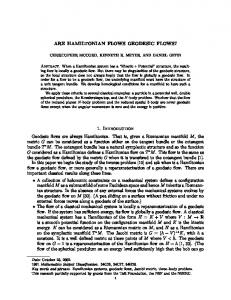
Fix a lift γ˜1 of γ1 parametrized so that γ˜1 (0) projects to γ1 (0) and lift the ˜ with h(1, ˜ ⋅) = γ˜1 ([0, T1 ]). The lift γ˜2 desired is given homotopy h to a homotopy h ˜ ⋅). by the (properly parametrized) geodesic h(0, The following lemma allows us to show that geodesic segments which are close after a time change are in fact close without the time change. This is where the assumption that the geodesic flow is on a space of negative curvature is used. The proof requires only that geodesics in the universal cover are globally length minimising, so a non-positive curvature assumption would be sufficient. Proposition 3.2. Let X be a CAT(−1) space, and γ1 , γ2 ∈ GX be geodesics. Suppose there exists a time change ρ ∶ [0, T2 ] → [0, T1 ] so that dX (γ1 (ρ(t)), γ2 (t)) < ǫ for all t ∈ [0, T2 ]. Then d(γ1 (t), γ2 (t)) < 3ǫ for all t ∈ [0, T1 − 2ǫ]. Proof. First, using Lemma 3.1, we lift γi to geodesic segments on the universal cover so that dX˜ (˜ γ1 (ρ(t)), γ˜2 (t)) < ǫ for all t ∈ [0, T2 ]. If we prove the statement in the universal cover, we have proven it in the original space. In the universal cover, the geodesics are globally length minimizing, and dX˜ (˜ γi (t1 ), γ˜i (t2 )) = ∣t1 − t2 ∣. We fix t ∈ [0, T2 ], and we know that γ˜2 (t) is within distance ǫ of γ˜1 (ρ(t)). Then one can reach γ˜2 (t) from γ˜2 (0) by the geodesic γ˜2 , or by following the path γ˜2 (0) → γ˜1 (0) → γ˜1 (ρ(t)) → γ˜2 (t) (see Figure 1). By the length-minimizing property of γ˜2 , t = dX˜ (˜ γ2 (0), γ˜2 (t)) < 2ǫ + dX˜ (˜ γ1 (0), γ˜1 (ρ(t))) = 2ǫ + ρ(t).

γ˜2 (0)

t

r ⎧ ⎪ ⎪ 0 be so small that dY (y1 , y2 ) < δ implies dGX (h(y1 ), h(y2 )) < ǫ/3K. Thus, writing γ1 = h(y1 ), γ2 = h(y2 ), it follows from Lemma 2.11 that dX (γ1 (0), γ2 (0)) < ǫ/3. Fix lifts {(yi , tî )}ki=1 under h of orbit segments {(g−T γi , ti + 2ǫ + 2T )}ki=1 . That is, each (yi , tî ) is an orbit segment for (Y, φt ) such that {h(φs yi ) ∶ s ∈ [0, tî ]} = {gs γi ∶ s ∈ [−T, ti + T + 2ǫ]}.

The first step is to apply the specification property to these lifted orbit segments. Let τˆ be provided by the weak specification property for (Y, φt ) at scale δ. There is a point z ∈ Y and a sequence of transition times τˆ1 , . . . τˆk−1 ≤ τˆ such that dtˆj (φsˆj−1 +ˆτj−1 z, yj ) < δ for every 1 ≤ j ≤ k,

where sˆj = ∑ji=1 tî + ∑j−1 î . Fix an index j, and write z ′ = φsˆj−1 +ˆτj−1 z. Consider the i=1 τ image under h of the orbit segment (z ′ , tˆj ). Then for all s ∈ [0, tˆj ], dGX (h(φs z ′ ), h(φs yj )) < ǫ/3K.

Thus, writing h(z ′ ) = γ ′ and reparameterizing, we see there is a time change ρ so that for all s ∈ [0, tj + 2ǫ + 2T ], dGX (gρ(s) γ ′ , gs (g−T γj )) < ǫ/3K.

Using Lemma 2.11, we see that for all s ∈ [0, tj + 2ǫ + 2T ], dX (γ ′ (ρ(s)), g−T γj (s)) < ǫ/3.

Now we apply Proposition 3.2 to obtain that for all s ∈ [0, tj + 2T ] dX (γ ′ (s), g−T γj (s)) < ǫ.

Now we apply Lemma 2.12 to obtain that for all s ∈ [T, tj + T ], and thus for all s ∈ [0, tj ],

dGX (gs γ ′ , gs (g−T γj )) < 2ǫ,

dGX (gs (gT γ ′ ), gs (γj )) < 2ǫ.

Now consider γ = gT (h(z)). Noting that gT γ ′ is an appropriate iterate of γ under (GX, gt ), the argument above shows that for each j, an appropriate iterate of γ is 2ǫ-shadowing for (γj , tj ). It only remains to show that the transition times for γ remain controlled. An argument based on continuity of the orbit equivalence and compactness of the phase space shows that there exists κ so that for all y ∈ Y , the image of an orbit segment (y, τˆ) under the orbit equivalence h is contained in the orbit segment (h(y), κ). That is, h({φs (y) ∶ s ∈ [0, τˆ]}) ⊆ {gs (h(y)) ∶ s ∈ [0, κ]}.

The details of this argument are given in §7.2. The segments of γ that correspond to transitions between the shadowed orbit segments comprise of images of orbit segments of the form (y, τî ) with τî ≤ τˆ, and an additional run of length at most 2T coming from the application of Lemma 2.12. Thus the transition times are bounded above by κ + 2T . It follows that (GX, gt ) satisfies weak specification.

14


4. CAT(0) spaces and codings for the geodesic flow In this section, we consider the case of non-positive curvature, and we prove Theorem 1.3 and Corollary 1.4.

4.1. Specification for a class of CAT(0) spaces. Theorem 1.3 states that if X is a compact, locally CAT(0), geodesic metric space with non-elementary fundamental group and topologically transitive geodesic flow, and there exists an orbit semiequivalence h ∶ Susp(Σ, T ) → GX, where (Σ, T ) is a compact subshift of finite type, then the geodesic flow on GX satisfies the weak specification property. We observe that this follows from our proof of Theorem 1.1, where we used the assumption of CAT(−1) in only two places; the first was to provide the orbit-equivalent symbolic description of GX (Lemma 2.8), which we now assume to hold; the second was in the proof of Proposition 3.2 and we already observed that a CAT(0) assumption was sufficient for that argument. We conclude that our proof of Theorem 1.1 also gives the statement of Theorem 1.3. A class of examples that is covered by Theorem 1.3 is given by CAT(0) spaces whose geodesics can be mapped homeomorphically to the geodesics for a CAT(−1) metric. For example, on a Riemannian surface with genus at least 2, non-positive curvature metrics can be found so that a single closed geodesic has curvature zero, and geodesics can be mapped homeomorphically to those for a hyperbolic metric. We note that even for these CAT(0) geodesic flows where the specification property holds, extensions of the dynamical properties of Theorem 1.2 would still require a great deal of new theory: our proofs will require Bowen regularity of the potentials under consideration, and the argument for H¨ older regularity to imply Bowen regularity (Propostion 5.4) requires negative curvature globally.

4.2. Non-existence of symbolic coding. We establish Corollary 1.4: if X is a complete, locally CAT(0), geodesic metric space with topologically transitive geodesic flow containing a geodesic γ, and there exists w > 0 such that some w˜ splits isometrically as R × Y , then there neighborhood Nw (˜ γ ) of a lift of γ to X does not exist any orbit semi-equivalence h ∶ Susp(Σ, T ) → GX, where (Σ, T ) is a compact shift of finite type. The idea is to show that the weak specification property does not hold for these geodesic flows, and we can thus conclude that it has no orbit semi-equivalent symbolic coding. We note that in many cases, there is a more elementary way to rule out the existence of a symbolic coding: if GX has uncountably many closed geodesics, since Susp(Σ, T ) has only countably many periodic orbits, a symbolic coding is impossible. So, for example, if X is the surface given by gluing together two tori using a flat cylinder, this simpler argument suffices. However, we note that having uncountably many closed geodesics is not a consequence of our hypotheses, even for Riemannian 3-manifolds. For example, the flat strip could have holonomy an irrational rotation around a single central closed geodesic. A construction like this requires dimension at least three. In dimension two, the main theorem of [CX08] implies that whenever a zero curvature neighborhood U of a geodesic in the universal cover exists, there is always a closed flat cylinder in the surface, allowing the simpler argument.


15

Proof of Corollary 1.4. Suppose that (GX, gt ) satisfies the weak specification propw , and let τ (δ) be the erty. Let K be as provided by Lemma 2.11, let δ = 10K corresponding maximum gap size. Let γ1 = γ and γ2 be a geodesic with γ2 (0) ∉ Nw (γ). Let t1 = τ and t2 = 1. For the weak specification property to hold in GX, there must be some geodesic γ ∗ which δ-shadows γ for time t1 , then after transition time at most τ , δ-shadows γ2 . By Lemma 2.11, d(γ(t), γ ∗ (t)) < Kδ = w/10 for all t ∈ [0, t1 ]. By the geometry of the flat neighborhood Nw (γ) (or, lifting to the universal cover, the flat strip Nw (˜ γ )), γ ∗ (t) travels at most distance w/5 perpendicular to the image of γ over t ∈ [0, t1 ], remaining all the while in the w/10-neighborhood of γ. Therefore, over the subsequent τ = t1 units of time, it can again travel at most distance w/5 perpendicularly away from the image of γ. Therefore at any time t ∈ [τ, 2τ ], γ ∗ (t) is at least distance w/5 from γ2 (0). To fulfill the desired shadowing, for some such w . Using t, gt γ ∗ should be within δ of γ2 . At such a time, dGX (gt γ ∗ , γ2 ) < δ = 10K w ∗ Lemma 2.11, we must at this point have d(γ (t), γ2 (0)) < Kδ = 10 . Since this is not the case, we have a contradiction and γ ∗ cannot achieve the shadowing required. We have shown that (GX, gt ) cannot have the weak specification property. Now suppose that there were an orbit semi-equivalence h ∶ Susp(Σ, T ) → GX, where (Σ, T ) is a compact shift of finite type. Then by §7.3, (Σ, T ) could be taken to be topologically transitive and the arguments of §3 would show that (GX, gt ) has weak specification. Therefore, no such h ∶ Susp(Σ, T ) → GX exists. One of the hypotheses of Corollary 1.4 is that the geodesic flow on M is topologically transitive. By [Bal95, Theorem III.2.4], if the geodesic flow is not topologically ˜ is contained in a flat plane. In the Riemannian case, transitive, every geodesic of X by [Ebe96, Prop 4.7.3 and 4.7.4], if M is rank one, the geodesic flow is transitive. If M is not rank one, then as noted above, every geodesic belongs to a flat plane. By the rank rigidity theorem [Bal85, BS87], M is a locally symmetric space of non-compact type, since we have assumed it is irreducible. But γ˜ has a flat neighborhood, implying M is flat, contradicting the irreducibility assumption. We remark that if M is flat, it will have uncountably many closed geodesics, which immediately rules out the existence of a symbolic coding. Remark. Corollary 1.4 rigorously confirms the expected phenomenon that a compact shift of finite type can not capture the dynamics of this setting. The idea of using the failure of the specification property to rule out the existence of a coding by a shift of finite type was first used by Lind [Lin79], who used this argument to show that quasi-hyperbolic toral automorphisms (i.e. ergodic automorphisms of the torus with some eigenvalues of modulus 1) do not admit Markov partitions. Beyond uniform hyperbolicity, the best hope to capture the dynamics symbolically is often to code using a shift of finite type on a countable alphabet. The existence of countable state symbolic dynamics for smooth flows on three dimensional Riemannian manifolds was recently established by Lima and Sarig [LS14]. This kind of phenomenon is not ruled out by Corollary 1.4. Remark. The work of Coornaert and Papadopoulos on existence of an orbit semiequivalent symbolic coding holds if π1 (X) is a hyperbolic group. However, it pro¯ vides a symbolic description of the geodesic flow on the group G(Γ) rather than GX (see proof of Lemma 2.8). This does not extend to GX under only a CAT(0)

16


assumption because a flat strip of parallel geodesics in X will correspond to a single ¯ geodesic in G(Γ). 5. Expansivity and the Bowen property Before turning to applications of the weak specification property, we require two further properties of the geodesic flow on a compact CAT(−1) space. The first property we want to check is expansivity (see [BW72]). Definition 5.1. A continuous flow {ft } on X is expansive if there is for all ǫ > 0, there exists δ > 0 such that for all x, y ∈ X and all continuous τ ∶ R → R with τ (0) = 0, if d(ft (x), ft (y)) < ǫ for all t ∈ R, then y = fs (x) for some s, where ∣s∣ < ǫ. That this property is satisfied by geodesic flows on a CAT(−1) space is not hard to see: Proposition 5.2. (GX, gt ) is expansive.

˜ let Proof. First, for a fixed geodesic γ˜ in X,

Opp(˜ γ ) = {˜ γ ′ ∶ γ˜ ′ (t) = γ˜(−t + s), for some s and all t}.

That is, Opp(˜ γ ) is the set of all linear reparametrizations of γ˜ with the opposite orientation. Let δ = minγ˜ ′ ∈Opp(˜γ ) dGX˜ (˜ γ , γ˜ ′ ). Using the definition of dGX˜ it is easy to check that δ does not depend on γ˜ and is positive. Take ǫ smaller than δ and smaller than ǫ0 /K (K from Lemma 2.11 and ǫ0 from Corollary 2.10). Consider any τ ∶ R → R with τ (0) = 0. Suppose that γ1 and γ2 are geodesics in GX with dGX (gt γ1 , gτ (t) γ2 ) < ǫ for all t. Then by Lemma 2.11, d(γ1 (t), γ2 (τ (t))) < Kǫ which is less than ǫ0 . Using Lemma 3.1, we can lift the geodesics γ1 and γ2 to the universal cover in such a way that d(˜ γ1 (t), γ˜2 (τ (t))) < Kǫ < ǫ0 for all t. Using the length-minimizing ˜ and the triangle inequality: properties of geodesics in X d(˜ γ1 (0), γ˜1 (t)) − 2ǫ0 < d(˜ γ2 (0), γ˜2 (τ (t))) < d(˜ γ1 (0), γ˜1 (t)) + 2ǫ0 .

Examining this inequality for t > 0 (resp. t < 0), we conclude that ∣τ (t)∣ → ∞ as t → ∞ (resp. as t → −∞). Together with the fact that d(˜ γ1 (t), γ˜2 (τ (t))) < ǫ0 for all t, this implies that γ˜2 (+∞), γ˜2 (−∞) ∈ {˜ γ1 (∞), γ˜1 (−∞)}. Since the endpoints at infinity for γ˜2 must be distinct, γ˜2 has the same pair of endpoints at infinity as γ˜1 . Since both are unit-speed geodesics, we have γ˜2 (t) = γ˜1 (±t + s) for some s. Now the assumption that τ (0) = 0 implies that dGX˜ (˜ γ1 , γ˜2 ) < δ and, by the choice of δ, that γ˜2 does not belong to Opp(˜ γ1 ). Hence γ˜2 (t) = γ˜1 (t + s) for some s. A straightforward calculation with the definition of dGX implies that ∣s∣ < ǫ. The second property we want is a dynamical regularity property for functions on the space GX. Definition 5.3 (see [Fra77]). Let {ft } be a continuous flow on a compact metric space (X, d). A continuous function ϕ on X is said to have the Bowen property (for φt ) if there exists V > 0 so that for any sufficiently small ǫ > 0, d(ft (x), ft (y)) < ǫ for all t ∈ [0, S] implies ∣ ∫ for any x, y ∈ X and any S > 0.

S 0

ϕ(ft x)dt − ∫

0

S

ϕ(ft y)dt∣ < V


17

We claim that H¨ older functions on GX satisfy this property. Proposition 5.4. If ϕ is a H¨ older continuous function on GX, then ϕ satisfies the Bowen property for the geodesic flow gt . Proof. We actually prove the Walters property for ϕ: for any V > 0, there exists an ǫ > 0 such that dGX (gt (γ1 ), gt (γ2 )) < ǫ for all t ∈ [0, S] implies ∣ ∫

S 0

ϕ(gt γ1 )dt−∫

S

0

ϕ(gt γ2 )dt∣ < V

for any γ1 , γ2 ∈ GX and any S > 0. Clearly, if ϕ has the Walters property, then ϕ has the Bowen property. The basic idea of the proof is that, using the CAT(−1) property for a comparison with H2 , geodesics in X which stay close over [0, S] are in fact exponentially close over that range, from which the result follows. The need to move between the metrics on GX and X adds some technicalities to the proof. Let V > 0 be given, and let C, α > 0 be the H¨ older constants for ϕ so that ∣ϕ(γ1 , γ2 )∣ < CdGX (γ1 , γ2 )α . We fix ǫ > 0 to be specified later. Suppose that dGX (gt γ1 , gt γ2 ) < ǫ for t ∈ [0, S]. By Lemma 2.11, dX (γ1 (t), γ2 (t)) < Kǫ for t ∈ [0, S]. By Lemma 3.1, assuming that Kǫ < ǫ0 , lifting to the universal cover, we have dX˜ (˜ γ1 (t), γ˜2 (t)) < ǫ for t ∈ [0, S]. We construct a comparison pair of geodesic segments c1 (t), c2 (t) in H2 with lengths S and with distance at most Kǫ between their endpoints using the pair of triangles shown in Figure 2. By convexity of the distance function, dH2 (c1 (t), c2 (t)) < Kǫ. We translate the time parameter for c2 by a constant r so that at the point of their nearest approach in H2 , both have the same time parameter. By interchanging the roles of c1 and c2 if necessary, we can assume that r ≥ 0. Since the flow is unit speed, r ≤ Kǫ, and we write S ′ ∶= S − r. Then, by a standard argument for the behavior of geodesics in H2 , we have that dH2 (c1 (t), c2 (t + r)) < Kǫe− min{t,S −t} for all t ∈ [0, S ′ ]. ′

Applying the CAT(−1) property, we have that

dX˜ (˜ γ1 (t), γ˜2 (t + r)) < Kǫe− min{t,S −t} for all t ∈ [0, S ′ ], ′

and we can push this estimate back down to X. ˜ X

H2 c1

γ˜1 qr γ˜2

p¯ r1

p1 r q¯ r p2 c2 (r) r

c2

r r p¯2

Figure 2. Comparison quadrilateral for Proposition 5.4. By the CAT(−1) condition, dX (p1 , p2 ) ≤ dH2 (¯ p1 , p¯2 ).

c1 (S ′ ) r

18


Next, using Lemma 2.12 we see that that there is a constant T = T (2Kǫ) such that dGX (gt γ1 , gt+r γ2 ) < 2dX (γ1 (t), γ2 (t + r)) < 2Kǫe− min{t,S −t} for all t ∈ [T, S ′ − T ]. ′

We recall from Lemma 2.12 that for small ǫ, we can take T (2Kǫ) = − log(2Kǫ), and thus limǫ→0 ǫα T (2Kǫ) = 0. We assume ǫ is so small that 2C(2Kǫ)α T < V /3. S S To control ∣ ∫0 ϕ(gt γ1 )dt − ∫0 ϕ(gt γ2 )dt∣, we first note that ∣∫

S

0

ϕ(gt γ1 )dt − ∫

S


S′

0

S′

ϕ(gt γ2 )dt∣ ≤ ∣ ∫

0


r

S

ϕ(gt γ2 )dt∣ + 2r∥ϕ∥.

Therefore, picking ǫ so small that 2Kǫ∥ϕ∥ < V /3, and writing γ2′ = gr γ2 , it suffices S′ S′ to control ∣ ∫0 ϕ(gt γ1 )dt − ∫0 ϕ(gt γ2′ )dt∣. We cover [0, S ′ ] by the intervals I1 = [0, T ], I2 = (T, S ′ − T ), and I3 = [S ′ − T, S ′ ]. Note that I2 may be empty and I1 and I3 may overlap, depending on the values of S ′ and ǫ. Then, ∣∫

S′ 0

0

S′

ϕ(gt γ2′ )dt∣ ≤ ∫

0

∣ϕ(gt γ1 ) − ϕ(gt γ2′ )∣dt

≤ ∫ ∣ϕ(gt γ1 ) − ϕ(gt γ2′ )∣dt + ∫ ∣ϕ(gt γ1 ) − ϕ(gt γ2′ )∣dt I3

I1

+∫

I2

∣ϕ(gt γ1 ) − ϕ(gt γ2′ )∣dt.

Over I1 and I3 , dGX (gt γ1 , gt γ2′ ) < dGX (gt γ1 , gt γ2 ) + dGX (gt γ2 , gt γ2′ ) < ǫ + Kǫ, so by the H¨ older condition, ∣ϕ(gt γ1 ) − ϕ(gt γ2′ )∣ ≤ C(2Kǫ)α . Thus ′ α ′ ∫ ∣ϕ(gt γ1 ) − ϕ(gt γ2 )∣dt + ∫ ∣ϕ(gt γ1 ) − ϕ(gt γ2 )∣dt < 2C(2Kǫ) T < V /3. I3

I1

To bound the integral over I2 , we use the H¨ older property again to obtain ′ α ′ ∫ ∣ϕ(gt γ1 ) − ϕ(gt γ2 )∣dt < ∫ CdGX (gt γ˜1 , gt γ˜2 ) dt I2

I2

< ∫ C2α K α ǫα e−α min{t,S−t} dt I2

0, there is a constant Q = Q(ρ) > 1 such that for every x ∈ X and t ∈ R, we have (6.1)

Q−1 e−tP (ϕ)+Φ(x,t) ≤ µ(Bt (x, ρ)) ≤ Qe−tP (ϕ)+Φ(x,t),

where Φ(x, t) = ∫0 ϕ(fs x) ds and Bt (x, ρ) = {y ∶ d(fs x, fs y) < ρ for all s ∈ [0, t]}. In particular, a measure of maximal entropy has the Gibbs property if for all ρ > 0, there is a constant Q = Q(ρ) > 1 such that for every x ∈ X and t ∈ R, we have t

Q−1 e−th ≤ µ(Bt (x, ρ)) ≤ Qe−th ,

(6.2)

It follows immediately from Theorem 6.1, Theorem 1.1, Proposition 5.2 and Proposition 5.4 that Proposition 6.2. Every H¨ older continuous function ϕ on GX has a unique equilibrium state. In particular, the Bowen-Margulis measure is the unique measure of maximal entropy. Furthermore, these measures satisfy the Gibbs property. 6.2. Equidistribution of weighted periodic orbits. Let Per(t) denote the set of closed orbits for {gs } of least period at most t, and let ϕ be a continuous function. We define the Gurevic pressure to be 1 (6.3) PG (ϕ) = lim sup log ∑ eΦ(γ) , t→∞ t γ∈Per(t) where Φ(γ) is the value given by integrating ϕ around the periodic orbit. It is easy to verify that in (6.3) we can instead sum over the set of periodic orbits of length between t and t + δ, for any fixed δ > 0. The pigeonhole principle yields the same upper exponential growth rate as in (6.3). For γ ∈ Per(t), let µ(γ) be the natural measure around the orbit. That is, if γ has period t, then 1 t µγ ∶= ∫ δgs γ ds. t 0 We say the periodic orbits weighted by ϕ equidistribute to a measure µ if 1 Φ(γ) µγ → µ, (6.4) ∑ e C(t) γ∈Per(t) where C(t) is the normalizing constant ∑γ∈Per(t) eΦ(γ) µγ (GX). Equidistribution of weighted periodic orbits for equilibrium states was first investigated in a uniformly hyperbolic setting by Parry [Par88]. For CAT(−1) spaces, it is known that in the case ϕ = 0, periodic orbits equidistribute to the Bowen-Margulis measure [Rob03, Theorem 5.1.1], but the weighted case has not been considered and seems to require different techniques from those used in [PPS15, Rob03]. We recall that the topological pressure for an expansive flow is defined to be P (ϕ) = lim

t→∞

t 1 log sup { ∑ e∫0 ϕ(gt x) ∣ E is a (t, ǫ)-separated set} , t x∈E

where ǫ is an expansivity constant for the flow, and a set E is (t, ǫ)-separated if for every distinct x, y ∈ E we have y ∉ B t (x, ǫ). The proof of the Variational Principle [Wal82, Theorem 9.10] shows that if PG (ϕ) = P (ϕ), then since Per(t) is a sequence of (t, ǫ)-separated sets (for any


21

expansivity constant ǫ) whose growth rate well approximates the topological pres1 eΦ(γ) µγ is an equilibrium state for ϕ. sure, then any weak∗ limit of C(T ) ∑γ∈Per(T ) See Remark 3 of [GS14]. Thus if we know that PG (ϕ) = P (ϕ), and that ϕ has a unique equilibrium state µ, it follows immediately that the periodic orbits weighted by ϕ equidistribute to µ. To prove that PG (ϕ) = P (ϕ) for a H¨ older continuous ϕ, we first require a closing lemma for our setting. The idea is that for the suspension flow over a shift of finite type, an orbit segment can always be approximated by a periodic orbit. Using ideas similar to those used earlier in the paper, we show that this property passes to GX using the orbit semi-equivalence. Lemma 6.3. For all ǫ > 0, there exists R > 0 so that for any orbit segment (γ, t) for (GX, gt ), there exists γ ∗ ∈ Per(t + R) so that dt (γ, γ ∗ ) < ǫ. Proof. The proof uses many of the same ideas as the proof of Theorem 3.3. Let ǫ > 0 be given and fix an orbit segment (γ, t) for (GX, gt ). Let h ∶ Y → GX be the orbit semi-equivalence provided by Lemma 2.8, where (Y, φt ) = Susp(Σ, T ) and Σ is a topologically transitive shift of finite type. Let K and T = T (ǫ) be the constants from Lemma 2.11 and Lemma 2.12 respectively, and let δ > 0 be so small that dY (y1 , y2 ) < δ implies dGX (h(y1 ), h(y2 )) < ǫ/3K. Fix a lift (y, tˆ) under h of (g−T γ, t + 2ǫ + 2T ), so {h(φs y) ∶ s ∈ [0, tˆ]} = {gs γ ∶ s ∈ [−T, t + T + 2ǫ]}.

On the suspension flow, it is easy to check that we can close orbit segments to ˆ so that for all (y, tˆ), there periodic orbits. That is, for all δ > 0, there exists R ′ ′ ′ ˆ This exists y so that dt (y, y ) < δ and y is periodic with period at most tˆ + R. ′ property follows from the corresponding fact for Σ. We take such a point y for the orbit segment (y, t) and δ > 0 under consideration. Then for all s ∈ [0, tˆ], dGX (h(φs y ′ ), h(φs y)) < ǫ/3K.

Thus, writing γ ′ ∶= h(y ′ ) and reparameterizing, we see there is a time change ρ so that for all s ∈ [0, t + 2ǫ + 2T ], dGX (gρ(s) γ ′ , gs (g−T γ)) < ǫ/3K.

Using Lemma 2.11, we see that for all s ∈ [0, t + 2ǫ + 2T ], dX (γ ′ (ρ(s)), g−T γ(s)) < ǫ/3.

Now we apply Proposition 3.2 to obtain that for all s ∈ [0, t + 2T ] dX (γ ′ (s), g−T γ(s)) < ǫ.

Now we apply Lemma 2.12 to obtain that for all s ∈ [T, t + T ], dGX (gs γ ′ , gs (g−T γ)) < 2ǫ,

and thus for all s ∈ [0, t], dGX (gs (gT γ ′ ), gs (γ)) < 2ǫ. We let γ ∗ = gT γ ′ , and we have shown that dt (γ ∗ , γ) < 2ǫ. Now it is clear that γ ∗ is a periodic orbit, so it only remains to show that its period is controlled. Let t∗ be the period of γ ∗ . We observe that the orbit segment (gt γ ∗ , t∗ − t) is a subset of the image under h of the orbit segment (φtˆy ′ , R′ ). So we let R be a value so that for all y ∈ Y , the image of an orbit segment (y, R′ ) under the orbit equivalence h is contained in the orbit segment (h(y), R). This is

22


possible by the compactness argument given in §7.2. Thus, the period of γ ∗ is at most t + R, so at scale 2ǫ, we have verified the property that we need.

Lemma 6.4. For any H¨ older continuous function ϕ ∶ GX → R, we have PG (ϕ) = P (ϕ).

Proof. Let 2ǫ be an expansivity constant. Since Per(t) is (t, 2ǫ)-separated, it is clear that PG (ϕ) ≤ P (ϕ). For the other inequality, take a sequence of (t, 2ǫ)-separated sets Et so that t 1 log ∑ e∫0 ϕ(gs x) → P (ϕ). t x∈Et Then by Lemma 6.3, for each x ∈ Et , there exists a periodic orbit γ(x) with dt (x, γ(x)) < ǫ and {γ(x) ∣ x ∈ Et } ⊂ Per(T + R). Since Et is (t, 2ǫ)-separated, if x ≠ y then γ(x) ≠ γ(y). Note that ∣Φ(γ(x)) − ∫

t

0

ϕ(gs x)∣ ≤ ∣∫

t

0

ϕ(gs γ(x)) − ∫

0

t

ϕ(gs x)∣ + R∥ϕ∥ ≤ V + R∥ϕ∥,

where V is the constant appearing in the Bowen constant for ϕ. Thus, ∑

γ∈Per(t+R)

and so

eΦ(γ) ≥

∑

eΦ(γ) ≥ e−V −R∥ϕ∥ ∑ e∫0

t

{γ(x)∣x∈Et}

ϕ(gs x)

,

x∈Et

t ⎞ V + R∥ϕ∥ t ⎛1 1 log log ∑ e∫0 ϕ(gs x) − . eΦ(γ) ≥ ∑ t+R t+R ⎝t t+R ⎠ x∈Et γ∈Per(t+R)

Taking a limit as t → ∞, we obtain PG (ϕ) ≥ P (ϕ), which completes the proof.

In summary, for any H¨ older continuous ϕ ∶ GX → R, since PG (ϕ) = P (ϕ) and ϕ has a unique equilibrium state µϕ , it follows that the periodic orbits weighted by ϕ are equidistributed in the sense that 1 Φ(γ) µγ → µϕ . ∑ e C(t) γ∈Per(t) This result holds true by the same proof if ϕ ∶ GX → R has the Bowen property.

6.3. Large Deviations Principle for the Bowen-Margulis measure and other equilibrium states. We obtain the large deviations principle for all the measures considered in this section, in particular the Bowen-Margulis measure. The large deviations principle is a statement which describes the decay rate of the measure of points whose Birkhoff sums are experiencing a large deviation from their expected value (given by the Birkhoff ergodic theorem). Definition 6.5. Let m be an equilibrium measure for a potential ϕ (with respect to F ). We say that m satisfies the upper large deviations principle if for any continuous observable ψ∶ X → R and any ǫ > 0,we have 1 t 1 (6.5) lim sup log m {x ∶ ∣ ∫ ψ(fs x) ds − ∫ ψ dm∣ ≥ ǫ} ≤ −q(ǫ), t 0 t→∞ t where the rate function q is given by (6.6)

q(ǫ) ∶= P (ϕ) −

sup

ν∈MF (X) ∣∫ ψ dm−∫ ψ dν∣≥ǫ

(hν (f ) + ∫ ϕ dν) ,


23

or q(ǫ) = ∞ when {ν ∈ MF (X) ∶ ∣∫ ψ dm − ∫ ψ dν∣ ≥ ǫ} = ∅. We say that the lower large deviations principle holds if the above statement holds with ≥ in place of ≤, and lim inf in place of lim sup in (6.5). We say that m satisfies the large deviations principle if both upper and lower large deviations hold: that is, the above statement holds with equality in place of ≤ in (6.5), and the lim sup becomes a limit. For a continuous map f , we say the lower large deviations principle holds (and similarly t for upper ) if the above statement holds with t replaced by n and 1t ∫0 ϕ(fs x) ds i replaced by ∑n−1 i=0 ϕ(f x) in (6.5), and MF (X) replaced by Mf (X) in (6.6). For a given function, the statement above is known as the level-1 large deviations principle. However, when this result applies to every continuous function, as we ask for in the definition above, it is equivalent to the level-2 large deviations principle [CRL11, Yam09]. We have the following result. Proposition 6.6. For every H¨ older continuous function ϕ on GX, the unique equilibrium state satisfies the large deviations principle. In particular, the BowenMargulis measure satisfies the large deviations principle for ϕ = 0. We now prove this result, treating the upper and lower large deviations bounds separately. 6.4. Upper large deviations. For the upper large deviations principle, we can reduce to considering the time-1 map of the flow. It is easy to see that the upper large deviations principle for the flow follows from the upper large deviations principle for the time-1 map. This follows because (6.5) can be verified for any continuous function ψ by applying the large deviations principle for the time-1 map to 1 the continuous function ψ1 ∶= ∫0 ψ(fs x)ds. The Gibbs property (6.1) for the flow immediately yields the Gibbs property with respect to the time-1 map. Q−1 e−tP (ϕ)+∑i=0

n−1

ϕ1 (f i x)

≤ µ(Bn (x, ρ; f1 )) ≤ Qe−tP (ϕ)+∑i=0

d1 (f1i x, f1i y)

n−1

ϕ1 (f i x)

,

where Bn (x, ǫ; f1 ) = {y ∶ < ρ for all i ∈ {0, . . . , n − 1}}, and d1 is the metric equivalent to d given by d1 (x, y) = supt∈[0,1) d(ft x, ft y). Note also that from the variational principle and flow invariance of the measure P (ϕ1 , f1 ) = P (ϕ, F ). It is well known that in the discrete time case the upper large deviations principle can be proved under the hypotheses of the upper Gibbs property and upper semicontinuity of the entropy map µ → hµ (which follows from expansivity of the flow). This follows from Theorem 3.2 of [PS05], whose hypotheses are the existence of an upper-energy function and upper semi-continuity of the entropy map. The existence of an upper-energy function eµ can easily be deduced from the upper bound in the Gibbs property (by setting eµ ∶= P (φ1 , f1 ) − φ1 (x)). See section 7.2 of [CT15] for this argument. Thus, we have the upper large deviations for ϕ1 for µ with respect to f1 , and thus the upper large deviations principle for ϕ with respect to the flow of (6.5). 6.5. Lower bounds. We now verify the lower large deviations principle. In the discrete time case, lower large deviations is proved as Theorem 3.1 of Pfister and Sullivan [PS05] under the following three hypotheses (see also Theorem 3.1 of [Yam09]): (1) Upper semi-continuity of the entropy map; (2) Existence of a “lower-energy function”, which follows easily from the lower Gibbs property;

24


(3) Entropy density of ergodic measures in the space of invariant measures. For a map f , the third hypothesis listed above, entropy density of ergodic measures, is the property that for any f -invariant measure µ, for any η > 0, we can find an ergodic measure ν such that D(µ, ν) < η and ∣h(ν) − h(µ)∣ < η, where D is the standard metric on the space of measures on X that is compatible with the weak∗ topology (see section 6.1 of [Wal82]). Entropy density is known to be true for maps with the almost product property [PS05], which is a weaker hypothesis than the specification property (the one with exact gaps). The basic argument was first proved for Zd -shifts with specification by Eizenberg, Kifer and Weiss [EKW94]. However, no reference is available for maps with weak specification, or for flows. In this section, we carefully prove entropy density for flows with weak specification. While this extension is expected, care must be taken in the argument, and dealing with the variable gap length is a nontrivial extension of the existing proofs. Remark. The time-1 map f1 of a flow with weak specification may not satisfy the entropy density condition: consider a suspension flow with roof function constant height 1. Each ergodic measure for f1 is supported on a single height, i.e on X ×{h} for some h ∈ [0, 1). Take an f1 -invariant measure given by a convex combination of an ergodic measure on X × {0}, and an ergodic measure on X × { 12 }. This measure can clearly not be approximated weak∗ by an ergodic f1 -invariant measure. Thus, for our lower large deviations argument, it is advantageous to work at the level of the flow rather than try to recover the result from the discrete time results. We prove that for a flow F = {ft } with weak specification and expansivity, the ergodic measures are entropy dense in the space of F -invariant measures. Proposition 6.7. Let F be an expansive flow with the weak specification property. Let µ be an F -invariant probability measure. Then for any η > 0, we can find an F-invariant ergodic measure ν such that D(µ, ν) < η and ∣h(ν) − h(µ)∣ < η. The strategy is to construct a closed F -invariant set Y ⊂ X such that every invariant measure supported on Y is weak*-close to µ, and such that the topological entropy of Y is close to h(µ). For x ∈ X and t ∈ R, define Et (x) ∶=

1 t δfs x ds. t ∫0 The measures Et (x) are sometimes called the empirical measures for the flow. Given a set U ⊂ MF (X), let Xt,U ∶= {x ∈ X ∣ Et (x) ∈ U }. From now on, we fix η > 0, and let B ∶= B(µ, 5η) and for m ≥ 1, let

(6.7)

Ym ∶= {x ∣ fs x ∈ Xm,B for all s ≥ 0}.

Each Ym is closed and forward invariant, so we can consider the dynamics of the semi-flow F + = {ft ∶ t ≥ 0} on Ym . We could modify the definition of Ym by replacing “s ≥ 0” with “s ∈ R” to get a flow-invariant set, but we avoid this to simplify the book-keeping of arguments that appear later in our proof. It is unproblematic to work with a set which is only forward invariant because measures which are invariant for F + ∣Ym can easily be shown to be invariant for F . More precisely, consider ν ∈ MF + (Ym ). Thinking of ν as a measure on X, then for each t ≥ 0,


25

ν ∈ Mft (X). Since ft is invertible, then ν is f−t invariant. Thus ν ∈ MF (X). We prove the following lemma. Lemma 6.8. For any m ≥ 1, if ν ∈ MF + (Ym ), then D(µ, ν) ≤ 6η.

Proof. Assume that ν ∈ MF + (Ym ) is ergodic. Since ν is ergodic, there exists a generic point x ∈ Ym , that is so Et (x) converges to ν. For a large value of t, we chop the orbit (x, t) into segments of length m (and a remainder), and use that for each i, fim x ∈ Xm,B . More precisely, for t ∈ R, write t = sm + q where s is an integer and 0 ≤ q < m. Then s−1

D(Et (x), µ) ≤ ∑

i=0

q m D(Em (fim x), µ) + D(Eq (fsm x), µ). t t

m Since D(Em (fim x), µ) ≤ 5η, we have ∑s−1 i=0 t D(Em (fim x), µ) ≤ 5η. For the remaining error term, writing M for the diameter of M(X), let t be large enough so that mM /t < η. Then D(Et (x), µ) < 6η. Thus, taking t → ∞, we have the lemma for ν ergodic. The result for ν non-ergodic follows from ergodic decomposition.

We will let Y ∶= YKn for values of K and n to be chosen shortly. By expansivity, the entropy map µ → h(µ) is upper semi-continuous. So by the variational principle and the fact that measures in Y are weak∗ -close to µ, then the topological entropy of Y cannot be much larger than h(µ); by choosing η small enough, we can guarantee that h(Y ) < h(µ) + γ. To show that Y has entropy close to h(µ), we use our specification property to build a large number of (t, ǫ)-separated points inside Y for arbitrarily large t, thus giving a lower bound on the topological entropy of Y . We rely on the following result, whose proof is a general argument based on the definition of entropy and the Birkhoff ergodic theorem. In the discrete time case, it is a corollary of Proposition 2.1 of [PS05] (see also Proposition 2.5 of [Yam09]). Proposition 6.9. Let µ be ergodic and h < h(µ). Then there exists ǫ > 0 such that for any neighborhood U of µ, there exists T so that for any t ≥ T there exists a (t, ǫ)-separated set Γ ⊂ Xt,U such that #Γ ≥ eth .

Now use the ergodic decomposition of µ to find λ = ∑pi=1 ai µi such that the µi are ergodic, the ai ∈ (0, 1) such that ∑pi=1 ai = 1, D(µ, λ) ≤ η, and h(λ) > h(µ) − η. See [You90] for a proof that this is possible. Let hi = 0 when h(µi ) = 0, and max(0, h(µi ) − η) < hi < h(µi ) otherwise. Take 3ǫi and Ti so that the conclusion of Proposition 6.9 holds for µi and hi , and let ǫ′ be the minimum of the ǫi , and T be the maximum of the Ti . Let Var(D, ǫ) ∶= sup{D(δx , δy ) ∣ d(x, y) < ǫ}.

Note that since the map x → δx is continuous, we have Var(D, ǫ) → 0 as ǫ → 0. Choose ǫ < ǫ′ so that Var(D, ǫ) < η. Choose t such that letting ti ∶= ai t, then ti ≥ T for every i. Note that t = ∑pi=1 ti . We are free to choose t as large as we like relative to p, and τ (ǫ), the maximum transition time provided by the weak specification property for F at scale ǫ. We will specify how large t needed to be chosen later in the proof. Let Ui = B(µi , η). Take (ti , 3ǫ)-separated sets Γi ⊂ Xti ,Ui such that #Γi ≥ eti hi . Now we use the weak specification property for the flow at scale ǫ to define a map ∞

Φ ∶ ∏(Γ1 × ⋯ × Γp ) → X. i=1

26


That is, given (x11 , . . . x1p , x21 , . . . , x2p , . . .), where xij ∈ Γj , we find a point y ∈ X which ǫ-shadows (x11 , t1 ), then after a transition period of time at most τ , ǫshadows (x12 , t2 ), and so on. Such a y can be found by the infinitary version of the weak specification property, see Lemma 7.1. We will show that the image of Φ is a subset of Y , and then use Φ to construct (t, ǫ)-separated sets for large t which satisfy cardinality estimates that yield the estimate we require on h(Y ). First we show that the image of Φ belongs to Y . The construction was chosen so that each time a portion of the orbit of y approximates a sequence of orbit segments in Γ1 × ⋯ × Γp , the orbit has spent exactly the right amount of time approximating each of µ1 , . . . , µp so that the appropriate empirical measure for y is close to µ. Thus, in what follows, we show that the empirical measures of y are close to µ along a subsequence corresponding to the times when y approximates a sequence in ∏ki=1 (Γ1 × ⋯ × Γp ). From there we bootstrap to all sufficiently large times. Fix a point y in the image of Φ, so y = Φ(x11 , . . . x1p , x21 , . . . , x2p , . . .), where xij ∈ Γj for all i ≥ 1, j ∈ {1, . . . , p}. Let τij (y) be the length of the transition time in the specification property that occurs immediately after approximating the orbit segment (xij , tj ). Let c = ∑pi=1 ti + (p − 1)τ : this is the upper bound on the total time taken to approximate a sequence of orbits in Γ1 × ⋯ × Γp . The precise time to approximate such a sequence of orbits for a point y is given by ck (y) = p p−1 k ∑i=1 ti + ∑i=1 τki (y). Let bk (y) = ∑i=1 (ci (y) + τip (y)), and b0 = 0. Then bk (y) is the total time that y spends approximating a sequence of orbits in ∏ki=1 (Γ1 × ⋯ × Γp ). Lemma 6.10. For all k ≥ 0, we have D(Ec (fbk (y) y), µ) ≤ 5η.

Proof. Fix k ≥ 1, and write y ′ = fbk−1 (y) y, τj = τkj (y), and si = ∑ij=1 tj + ∑i−1 j=1 τj , so si is the total time that y ′ initially spends approximating the corresponding sequence in Γ1 × ⋯ × Γi . Then, writing M for the diameter of MF (X) in the metric D, we remove the ‘uncontrolled’ portion of the orbit of y from consideration by using the estimate p ti p D (Ec (y ′ ), ∑ Eti (fsi−1 +τi−1 y ′ )) ≤ τ M. c c i=1 Now since dti (fsi−1 +τi−1 y ′ , xki ) < ǫ, for each i, we have

D (Eti (fsi−1 +τi−1 y ′ ), Eti (xki )) < ti Var(D, ǫ) < ti η.

Thus, by chosing t, and hence c, so large that pc τ M < η, we have p p ti ti Eti (xki )) < τ M + ∑ η < 2η. c c i=1 c i=1 p

D (Ec (y ′ ), ∑

Now since for each i, xki ∈ Xti ,Ui , we have p

p p ti ti ti Eti (xki ), ∑ µi ) ≤ ∑ η < η. c c i=1 i=1 i=1 c

D (∑

Furthermore, we have t ≤ c = ∑pi=1 ti + (p − 1)τ ≤ t + pτ , so if t is chosen to be much larger than pτ then ti /c is close to ti /t = ai and we can ensure that p ti Eti (xki ), ∑ ai µi ) < η. i=1 i=1 c p

D (∑


27

Putting all this together, we have p

p p ti ti ti Eni (xki )) + D (∑ Eti (xki ), ∑ µi ) c c i=1 i=1 i=1 c

D(Ec (fbk−1 y), µ) ≤ D (Ec (y ′ ), ∑

p p ti µi , ∑ ai µi ) + D (∑ ai µi , µ) < 5η. i=1 i=1 i=1 c p

+ D (∑

The previous lemma was where we required that t is large relative to τ and p. In the next lemma, we specify how large K needs to be chosen. The idea is that an orbit segment of y of length K(c + τ ) will comprise of K − 2 sub-segments of length c where Lemma 6.10 applies and so the empirical measures along the subsegments are close to µ. Additional deviation of the empirical measure along the whole orbit segment is made arbitrarily small by choosing K large. This is the strategy for the proof of the following lemma. Lemma 6.11. If y is a point in the image of Φ, then y ∈ Y . Proof. Given s ≥ 0, we need to show that fs y ∈ XKt,B for a suitably chosen K. The idea is that taking the unique m so that bm < s ≤ bm+1 , we have K−2

EKt (fs y) = ∑

i=1

c Ec (fbm+i y) + error. Kt

The error term has two sources. First, there are at most K segments of y’s orbit, each of length at most τ , used as the transition segments in the application of the specification property in the construction of Φ. Second, there is a run of length at most t + τ at both the start and end of the orbit segment (fs y, Kt). More precisely, using Lemma 6.10, we have c(K − 2) τK 2M (t + τ ) c τ M 2M 2M τ D(EKt (fs y), µ) ≤ 5η + M+ ≤ 5η + + + . Kt Kt Kt t t K Kt We see that if K and t are large enough, then the right hand side is arbitrarily small. Thus y ∈ YKt = Y . Now we prove our entropy estimates. We use Φ to define a map m

m ∏i=1 (Γ1

Φm ∶ ∏(Γ1 × ⋯ × Γp ) → Y. i=1

For each x ∈ × ⋯ × Γp ), we make a choice of y ∈ ∏∞ i=1 (Γ1 × ⋯ × Γp ) with yij = xij for i ∈ {1, . . . , m}, j ∈ {1, . . . , p}, and we define Φm (x) ∶= Φ(y). By Lemma 6.11, the image of Φm belongs to Y . For j ∈ {1, . . . , mp − 1}, let τj (x) ∈ [0, τ ] denote the jth transition time that occurs when applying the specification property in the definition of Φm (x). Lemma 6.12. There exists a constant C so that for all m, the image of Φm contains a (bm , ǫ/2)-separated set Em with #Em ≥ C −m # ∏m i=1 (Γ1 × ⋯ × Γp ).

Proof. Let k ∈ N be large enough so that, writing ζ ∶= τ /k, we have d(x, fs x) < ǫ/2 for every x ∈ X and s ∈ (−ζ, ζ). We partition the interval [0, mpτ ] into kmp subintervals I1 , . . . , Ikmp of length ζ, denoting this partition as P . Given x ∈ ∏m i=1 (Γ1 × ⋯ × Γp ), take the sequence n1 , . . . , nk so that τ1 (x) + ⋯ + τi (x) ∈ Ini for every 1 ≤ i ≤ mp − 1.

28


Now let l1 = n1 and li+1 = ni+1 −ni for 1 ≤ i ≤ k−2, and let l(x) ∶= (l1 , . . . , lk−1 ). Since τi+1 (x) ∈ [0, τ ], we have ni ≤ ni+1 ≤ ni + k for each i, so l(x) ∈ {0, . . . , k − 1}mp−1 . ¯ Now given ¯ l ∈ {0, . . . , k − 1}mp−1 , let Γl ⊂ ∏m i=1 (Γ1 × ⋯ × Γp ) be the set of all x ¯ ′ l ¯ such that l(x) = l. Note that if x, x ∈ Γ and i ∈ {1, . . . , k − 1}, then by construction, τ1 (x) + ⋯ + τi (x) and τ1′ (x) + ⋯ + τi′ (x) belong to the same element of the partition P. ¯ ¯ We show that Φm is 1-1 on each Γl . Fix ¯l and let x, x′ ∈ Γl be distinct. Let j be the smallest index such that xj ≠ x′j . Write τi = τi (x) and τi′ = τi (x′ ). Let r = ∑ji=1 (ti + τi ) and r′ = ∑ji=1 (ti + τi′ ). Since ∑ji=1 τi and ∑ji=1 τi belong to the same element of P , then ∣r − r′ ∣ = ∣ ∑ji=1 τi − ∑ji=1 τi′ ∣ < ζ. Because xj ≠ x′j ∈ Γi for some i ∈ {i, . . . , p} and Γi is (ti , 3ǫ)-separated, we have dti (xj , x′j ) > 3ǫ. Now we have dbm (Φm x, Φm x′ ) ≥ dti (fr Φm x, fr Φm x′ ) > dti (fr Φm x, fr′ Φm x′ ) − ǫ/2,

where the ǫ/2 term comes from the fact that dti (fr Φm x′ , fr′ Φm x′ ) ≤ ǫ/2 by our choice of ζ. For the first term, observe that dti (fr Φm x, fr′ Φm x′ ) ≥ dti (xj , x′j )−dti (xj , fr Φm x)−dti (fr′ Φm x′ , x′j ) > dti (xj , x′j )−2ǫ.

It follows that dbm (Φm x, Φm x′ ) > ǫ/2. Thus, Φm is 1-1 on Γl and Φm (Γl ) is (bm , ǫ/2)-separated. There are k mp−1 choices for ¯l, so letting C = k p , by the pi¯ geon hole principle, there exists ¯l so that #Γl ≥ C −m #(∏m i=1 Γ1 × ⋯ × Γp ). For this ¯ ¯l, we let Em ∶= Φm (Γl ). ¯

¯

We have that p

#Em ≥ C −m (∏ #Γi )m ≥ C −m em ∑i=1 ti hi ≥ C −m emt ∑i=1 ai hi e−m ∑i=1 hi p

p

p

i=1

log #Em > h(µ) − η + 1t (∑pi=1 hi + C). Taking a limit as m → ∞, and Thus, m → 1, this shows that h(Y ) > h(µ) − η. observing that btm Since h(Y ) = sup{h(ν) ∶ ν is ergodic and ν ∈ MF + (Y )}, we can find an ergodic measure ν supported on Y with h(ν) > h(µ) − η. The discussion preceding Lemma 6.8 shows that ν ∈ MF (X). Thus ν satisfies the conclusion of Proposition 6.7. 1 tm

Completing the proof of lower large deviations. Now that we have entropy density of ergodic measures, the rest of the argument is standard. Nevertheless, we do not know of a convenient reference in continuous time, so we sketch the proof. First observe that it is clear that entropy density of ergodic measures means that it is possible to consider only ergodic measures in the expression sup {hν (f ) + ∫ ϕdν ∶ ∣∫ ψ dm − ∫ ψ dν∣ ≥ ǫ} . Thus, for the lower large deviations, it will suffice to show is that for any ergodic µ with ∣∫ ψ dm − ∫ ψ dν∣ > ǫ and δ > 0 sufficiently small that 1 t 1 log m {x ∶ ∣ ∫ ψ(fs x) ds − ∫ ψ dµ∣ ≤ δ} ≥ P (ϕ) − (h(µ) + ∫ ϕdµ). t→∞ t t 0

(6.8) lim

This is achieved by a combination of the Gibbs property for m, and basic cardinality estimates for µ. A sketch goes as follows.


29

● For a suitable small η > 0, from the Katok entropy formula, and the Birkhoff ergodic theorem, we can find a sequence of (t, η) separated sets with #Et > et(h(µ)−η) so that for φ ∈ {ϕ, ψ} we have 1 t ∣ ∫ φ(fs x) ds − ∫ φ dµ∣ ≤ δ y∈Bt (x,η),x∈Et t 0 sup

● Then 1 t m {x ∶ ∣ ∫ ψ(fs x) ds − ∫ ψ dµ∣ ≤ δ} ≥ ∑ m(Bt (x, η)) t 0 x∈Et ● By the Gibbs property, m(Bt (x, η)) ≥ C −1 e−tP (ϕ)+∫0 ϕ(fs x)ds , and since t x ∈ Et , ∫0 ψ(fs x)ds ≥ ∫ tψdµ − tδ. ● Thus 1 t m {x ∶ ∣ ∫ ψ(fs x) ds − ∫ ψ dµ∣ ≤ δ} ≥ Q−1 #Et e−tP (ϕ)+tψdµ−tδ t 0 ≥ Q−1 e−t(P (ϕ)−(h(µ)+∫ ϕdµ)+η+δ) t

The proof of the lower large deviations principle follows. 7. Some technical results We provide details of some technicals results that we used earlier in the paper. 7.1. Finitary to infinitary specification. Lemma 7.1. Let F be a flow on a compact metric space X, and assume that F satisfies the weak specification property. Then the conclusion of the specification property also holds for any countably infinite sequence of orbit segments. Proof. Let δ > 0 be the scale, and τ > 0 the maximum gap size for the scale δ/3 provided by the weak specification property for F . It is clear from the definition that τ can also serve as a maximum gap size for the scale δ. Now let {(xi , ti )}i∈N be a countably infinite sequence of orbit segments. For each j ∈ N, we use the weak specification on the first j orbit segments {(xi , ti )}ji=1 (j) to produce a point yj ∈ X and corresponding transition times τi (1 ≤ i ≤ j), so that appropriate iterates of yj (δ/3)-shadow the prescribed orbit segments. Since the space X is compact, one can choose an accumulation point for the sequence {yj }j∈N , call it y. Passing to a subsequence, we may assume that yj → y. We now want to verify that y has the desired property. To do this, we need to produce a countable collection τi of transition times, and check the corresponding (j) specification property. First, look at the sequence {τ1 }j∈N ⊂ [0, τ ]. Passing to a (j) subsequence if necessary, we may assume {τ1 }j∈N converges to τ1 ∈ [0, τ ]. Next (j) consider the sequence {τ2 }j≥2,j∈N ⊂ [0, τ ]. Again, passing to a subsequence, we can choose a limiting τ2 ∈ [0, τ ]. Continuing in this manner, we obtain a sequence of transition times {τi }i∈N . Having defined the transition times, we now verify the infinitary specification condition. Given k ∈ N, we consider the finitely many orbit segments {(xi , ti )}ki=1 . By compactness, there is an ǫ > 0 with the property that, for any pair of points satisfying d(z, z ′ ) ≤ ǫ, we have dsk (z, z ′) < δ/3. By continuity of the flow, there is also an ǫ′ > 0 so that for all x ∈ X, ∣t − t′ ∣ < ǫ′ , and 1 ≤ i ≤ k, we have dti (ft (x), ft′ (x)) < δ/3.

30


We now choose a y ′ ∶= yN from the approximating sequence having the following (N ) two properties: (i) d(y ′ , y) < ǫ, and (ii) each ∣τi − τi ∣ < ǫ′ /k, for 1 ≤ i ≤ k. From property (i), we conclude that dsk (y, y ′ ) < δ/3, and from property (ii), it (N ) (N ) follows immediately that ∣(si + τi ) − (si + τi )∣ < ǫ′ holds for all 1 ≤ i ≤ k. We now have the estimate: dti (fsi−1 +τi−1 y, xi ) ≤ dti (fsi−1 +τi−1 y, fsi−1 +τi−1 y ′ ) + dti (fsi−1 +τi−1 y ′ , xi ) ≤ dsk (y, y ′ ) + dti (fsi−1 +τi−1 y ′ , xi )

≤ dsk (y, y ′ ) + dti (fsi−1 +τi−1 y ′ , fs(N ) +τ (N ) y ′ ) + dti (fs(N ) +τ (N ) y ′ , xi ) i−1

i−1

i−1

i−1

≤ δ/3 + δ/3 + δ/3 = δ. The first and third inequalities are just applications of the triangle inequality for the metric dti . The second inequality comes from the definition of the metrics dt , along with the fact that si−1 +τi−1 +ti ≤ sk for every 1 ≤ i ≤ k. For the last inequality, the first term is controlled by property (i), while the second term is controlled by property (ii) and the choice of ǫ′ . The last term is controlled by the specification property at scale δ/3 for the point y ′ = yN . This gives the desired estimate, and since this can be done for every k ∈ N, completes the proof. 7.2. A technical lemma for orbit equivalence. Let (X, φt ) and (Y, ψt ) be continuous flows on compact metric spaces. Let h ∶ X → Y be a continuous orbit semi-equivalence between φt and ψt . By continuity of the orbit semi-equivalence, an orbit segment (x, t) for (X, φt ) is mapped to an orbit segment (h(x), τ (x, t)) for (Y, ψt ). That is, h({φs (x) ∶ s ∈ [0, t]}) = {ψs (h(x)) ∶ s ∈ [0, τ (x, t)]},

and in particular, h(φt (x)) = ψτ (x,t)(h(x)).

Proposition 7.2. Let (X, φt ) and (Y, ψt ) be continuous flows on compact metric spaces, and suppose that (Y, ψt ) has no fixed points. Let h ∶ X → Y be a continuous orbit semi-equivalence between φt and ψt . Then the function τ ∶ X × R+ → R+ defined as above is continuous. Proof. It is clear from continuity of the orbit semi-equivalence that as s → t, τ (x, s) → τ (x, t), so it suffices to study the first coordinate and show that for a fixed t, if xk → x, then τ (xk , t) → τ (x, t). We fix ǫ > 0. Since the flow (Y, ψt ) has no fixed points, there exists δ > 0 so that if d(ψs1 y, ψs2 y) < δ, then ∣s1 − s2 ∣ < ǫ. Let τ ∶= τ (x, t). Then, by continuity of the flow and h, ψτ (h(xk )) → ψτ (h(x)). Thus, for k large, we have d(ψτ (h(xk )), ψτ (h(x))) < δ/2,

where d is the metric on Y . Now we consider the sequence h(φt xk ). By continuity, h(φt xk ) → h(φt x) = ψτ (h(x)). Thus, for k large, we have d(h(φt xk ), ψτ (h(x))) < δ/2,

and so we have d(ψτ (xk ,t) (h(xk )), ψτ (h(xk )) = d(h(φt xk ), ψτ (h(xk )) < δ, and these points are on the same orbit. Thus it follows that ∣τ (xk , t) − τ ∣ < ǫ. It follows that τ (xk , t) → (x, t), and thus the function τ is continuous.


31

Corollary 7.3. Let (X, φt ), (Y, ψt ), and h ∶ X → Y be as in Proposition 7.2. Then for all t, there exists K > 0, so that for all x ∈ X, the image of (x, t) under the orbit semi-equivalence h is contained in the orbit segment (h(x), K). That is, h({φs (x) ∶ s ∈ [0, t]}) ⊆ {ψs (h(x)) ∶ s ∈ [0, K]}.

Proof. By continuity of τ , and compactness of X × {t}, it follows that which proves the corollary.

sup{τ (x, t) ∶ x ∈ X} < ∞,

7.3. Topological transitivity and orbit equivalence. The following Lemma allows us to assume the coding provided by Lemma 2.8 is topologically transitive. Lemma 7.4. Let (Σ, T ) be a shift of finite type, and suppose that h ∶ Susp(Σ, T ) → (X, φ) is a continuous, surjective orbit equivalence onto a space without isolated points. Suppose that the flow φ on X is topologically transitive. Then there exists a topologically transitive subshift (Σ′ , T ∣Σ′ ) of (Σ, T ) which is still of finite type, and such that Susp(Σ′ , T ∣Σ′ ) maps surjectively onto (X, φ) via the restriction of h.

Sketch of proof. Using the language L of the shift (Σ, T ), we decompose its alphabet A as A = {non-essential symbols} ∪ ⋃ Ek k

where a symbol i is non-essential if iwi ∉ L for any word w, and where the Ek are equivalence classes of the relation: i ∼ j ⇐⇒ there exist words u, w such that iuj, jwi ∈ L

on the set of essential symbols. It is clear that for any element of Σ, all symbols of sufficiently large index lie in a single Ek . If we let Ek = {σ ∈ Σ ∶ σ(n) ∈ Ek for all n}, then the subshift (Ek , T ∣Ek ) is clearly topologically transitive and also of finite type. It is easy to check that for any σ ∈ Σ, d(T n σ, Ek ) → 0 for some (unique) k. Let x be a point of X whose orbit is dense in X. Since X has no isolated points, for any A, O(x, [A, ∞)) = {φt x ∶ t ∈ [A, ∞)} is also dense in X. Lift x to a point (σ, s) ∈ Susp(Σ, T ) and O(x, [A, ∞)) to O((σ, s), [B(A), ∞)). Since Susp(Σ, T ) is compact and h is continuous and surjective, it is closed. Hence, for arbitrarily large B, h(O((σ, s), [B, ∞)) = X. Now, as B → ∞, O((σ, s), [B, ∞)) limits on the suspension of one of the subshifts (Ek , T ). Using uniform continuity and closedness of h, it is now clear that h∣Susp(Ek ,T ∣Ek ) is an orbit equivalence mapping surjectively onto (X, φ). References [Adl98] [Bal85] [Bal95] [BD04] [BG11]

Roy L. Adler. Symbolic dynamics and Markov partitions. Bull. Amer. Math. Soc. (N.S.), 35(1):1–56, 1998. Werner Ballmann. Nonpositively curved manifolds of higher rank. Annals of Mathematics, 122(3):597–609, 1985. Werner Ballmann. Lectures on spaces of nonpositive curvature, volume 25 of DMV Seminar. Birkh¨ auser, Basel, 1995. Mike Boyle and Tomasz Downarowicz. The entropy theory of symbolic extensions. Invent. Math., 156(1):119–161, 2004. A.I. Bufetov and B.M. Gurevich. Existence and uniqueness of the measure of maximal entropy for the Teichm¨ uller flow on the moduli space of Abelian differentials. SB Math, 202(7):935–970, 2011.

32

[Bow72]


Rufus Bowen. Periodic orbits for hyperbolic flows. American Journal of Mathematics, 94(1):1–30, 1972. [Bow73] Rufus Bowen. Symbolic dynamics for hyperbolic flows. Amer. J. Math., 95:429–460, 1973. [Bow74] Rufus Bowen. Maximizing entropy for a hyperbolic flow. Math. Systems Theory, 7(4):300–303, 1974. [Bow75] Rufus Bowen. Some systems with unique equilibrium states. Mathematical Systems Theory, 8(3):193–202, 1975. [BR75] Rufus Bowen and David Ruelle. The ergodic theory of Axiom A flows. Inventiones Mathematicae, 29(3):181–202, 1975. [BS87] Keith Burns and Ralf Spatzier. Manifolds of nonpositive curvature and their buldings. ´ Inst. Hautes Etudes Sci. Publ. Math., (65):35–59, 1987. [BV15] Thiago Bomfim and Paulo Varandas. The gluing orbit property, uniform hyperbolicity and large deviations principles for semiflows. Available at ArXiv:1507.03905, 2015. [BW72] R. Bowen and P. Walters. Expansive one-parameter flows. J. Differential Equations, 12:180–193, 1972. [Cha94] Christophe Champetier. Petite simplification dans les groupes hyperboliques. Ann. Fac. Sci. Toulouse Math., 3(2):161–221, 1994. [CP12] Michel Coornaert and Athanase Papadopoulos. Symbolic coding for the geodesic flow associated to a word hyperbolic group. Manuscripta Math., 109:465–492, 2012. [CRL11] Henri Comman and Juan Rivera-Letelier. Large deviation principles for non-uniformly hyperbolic rational maps. Ergodic Theory Dynam. Systems, 31(2):321–349, 2011. [CT15] Vaughn Climenhaga and Daniel J. Thompson. Unique equilibrium states for flows and homeomorphisms with non-uniform structure. (Available at ArXiv:1505.03803), May 2015. [CX08] Jianguo Cao and Frederico Xavier. A closing lemma for flat strips in compact surfaces of non-positive curvature. (Unpublished. Available at http://citeseerx.ist.psu.edu/viewdoc/summary?doi=10.1.1.70.5005), 2008. [Den92] Manfred Denker. Large deviation and the pressure function. In Transactions of the 11th Prague Conference on Information theory, Statistical Decision Functions, Prague, 1990, pages 21–33. Springer, Berlin, 1992. [Ebe96] Patrick Eberlein. Geometry of nonpositively curved manifolds. Chicago Lectures in Mathematics. University of Chicago Press, Chicago, IL, 1996. [EKW94] A. Eizenberg, Y. Kifer, and B. Weiss. Large deviations for Zd -actions. Comm. Math. Phys, 164(3):433–454, 1994. [Fra77] Ernesto Franco. Flows with unique equilibrium states. Amer. J. Math., 99(3):486–514, 1977. [GM10] Katrin Gelfert and Adilson E. Motter. (Non)invariance of dynamical quantities for orbit equivalent flows. Comm. Math. Phys., 300(2):411–433, 2010. [Gro87] M. Gromov. Hyperbolic groups. In S. Gersten, editor, Essays in Group Theory, volume 8 of MSRI Publications, pages 75–265. Springer, 1987. [GS14] Katrin Gelfert and Barbara Schapira. Pressures for geodesic flows of rank one manifolds. Nonlinearity, 27(7):1575–1594, 2014. [Kai90] Vadim A. Kaimanovich. Invariant measures of the geodesic flow and measures at infinity on negatively curved manifolds. Ann. Inst. H. Poincar´ e Phys. Th´ eor., 53(4):361–393, 1990. Hyperbolic behaviour of dynamical systems (Paris, 1990). [Kai91] Vadim A. Kaimanovich. Bowen-Margulis and Patterson measures on negatively curved compact manifolds. In Dynamical systems and related topics (Nagoya, 1990), volume 9 of Adv. Ser. Dynam. Systems, pages 223–232. World Sci. Publ., River Edge, NJ, 1991. [KH95] Anatole Katok and Boris Hasselblatt. Introduction to the modern theory of dynamical systems. Cambridge University Press, 1995. [Kni98] Gerhard Knieper. The uniqueness of the measure of maximal entropy for geodesic flows on rank 1 manifolds. Ann. of Math., 148(1):291–314, 1998. [Kni05] Gerhard Knieper. The uniqueness of the maximal measure for geodesic flows on symmetric spaces of higher rank. Israel J. Math., 149:171–183, 2005. Probability in mathematics.


[Lin79]

[LS14] [Mat91] [Par88]

[PP90] [PPS15] [PS05] [Rob03] [Sar13] [Wal82] [Yam09] [You90]

33

D. A. Lind. Ergodic group automorphisms and specification. In Ergodic theory (Proc. Conf., Math. Forschungsinst., Oberwolfach, 1978), volume 729 of Lecture Notes in Math., pages 93–104. Springer, Berlin, 1979. Yuri Lima and Omri Sarig. Symbolic dynamics for three dimensional flows with positive topological entropy. (Available at ArXiv:1408.3427), 2014. Fr´ ed´ eric Math´ eus. Flot g´ eod´ esique et groupes hyperboliques d’apr´ es M. Gromov. In S´ eminaire de Th´ eorie Spectrale et G´ eom´ trie, number 9, pages 67–87. 1991. William Parry. Equilibrium states and weighted uniform distribution of closed orbits. In Dynamical systems (College Park, MD, 1986–87), volume 1342 of Lecture Notes in Math., pages 617–625. Springer, Berlin, 1988. W. Parry and M. Pollicott. Zeta functions and the periodic orbit structure of hyperbolic dynamics. Number 187-188 in Ast´ erisque. Soc. Math. France, 1990. Fr´ ed´ eric Paulin, Mark Pollicott, and Barbara Schapira. Equilibrium states in negative curvature. Ast´ erisque, (373):viii+281, 2015. C-E Pfister and W G Sullivan. Large deviations estimates for dynamical systems without the specification property. application to the β-shifts. Nonlinearity, 18:237–261, 2005. Thomas Roblin. Ergodicit´ e et ´ equidistribution en courbure n´ egative. M´ em. Soc. Math. Fr. (N.S.), (95):vi+96, 2003. Omri M. Sarig. Symbolic dynamics for surface diffeomorphisms with positive entropy. J. Amer. Math. Soc., 26(2):341–426, 2013. Peter Walters. An introduction to ergodic theory, volume 79 of Graduate Texts in Mathematics. Springer-Verlag, New York-Berlin, 1982. Kenichiro Yamamoto. On the weaker forms of the specification property and their applications. Proceedings of the AMS, 137(11):3807–3814, November 2009. L.S. Young. Large deviations in dynamical systems. Trans. Amer. Math. Soc., 318(2):525–543, 1990.

Wesleyan University, Mathematics and Computer Science Department, Middletown, CT 06459 Department of Mathematics, Ohio State University, Columbus, Ohio 43210 Department of Mathematics, Ohio State University, Columbus, Ohio 43210

THE WEAK SPECIFICATION PROPERTY FOR GEODESIC FLOWS ...

THE WEAK SPECIFICATION PROPERTY FOR GEODESIC FLOWS ...

Suggest Documents

ARE HAMILTONIAN FLOWS GEODESIC FLOWS?

On a generic property of geodesic flows - CiteSeerX

Geodesic Information Flows

Weak synchronization for isotropic flows

Weak Shadowing Property for IFS

From the transfer operator for geodesic flows on ... - TU Clausthal

Levi-Civita regularization and geodesic flows for the 'curved'Kepler

Noncommutative Integrability, Moment Map and Geodesic Flows ...

Jacobi vector fields of integrable geodesic flows

Integrable magnetic geodesic flows on Lie groups

Which geodesic flows are left-handed?

Integrable geodesic flows of non-holonomic metrics

Perturbations of geodesic flows by recurrent dynamics

Integrable geodesic flows of non-holonomic metrics

THE STRENGTH OF THE WEAK LEFSCHETZ PROPERTY

Singular solutions for geodesic flows of Vlasov moments

A PROPERTY ON GEODESIC MAPPINGS OF PSEUDOSYMMETRIC ...

The Maupertuis principle and geodesic flows on the ... - CiteSeerX

The Maupertuis principle and geodesic flows on the sphere arising

PROPERTY OF RECIPROCITY FOR STRATIFIED LAMINAR FLOWS ...

THE WEAK LEFSCHETZ PROPERTY AND POWERS OF

Laplace Equations and the Weak Lefschetz Property

SPECIFICATION PROPERTY AND ... - Semantic Scholar

projective structure and integrable geodesic flows on the extension of ...