develop different kinds of artificial creatures: assemblies of organs able to perform a .... adapted to artificial life because creature genome is small and the fitness ...
Three simulators for growing artificial creatures Sylvain Cussat-Blanc, Jonathan Pascalie, Herv´e Luga, Yves Duthen Abstract— Artificial embryogeny aims to develop a complete organism starting from a unique cell. For years, plenty of developmental models have been introduced. The main interests are reported on morphogen positioning, differentiation mechanisms and cellular interactions. In this paper, we show how the developmental model Cell2Organ has been extended to become a multi-level simulator able to work both on morphogen positioning thanks to an hydrodynamic layer and on cellular interaction with a physical layer. Through different experiments, we show the capacities of such a model with a “muscular joint” able to move in a physical world and a small organism able to create substrate vortices thanks to the hydrodynamic engine. The inspiration of such a set of simulators is provided the gastrulation stage of vertebrate embryos. During this stage, the embryo reorganizes its environment to continue its growth.
I. I NTRODUCTION Nowadays, many developmental models can produce different kinds of creatures starting from a single cell. With the aim to produce a complete ecosystem composed of various adapted creatures, many questions are still pending. One of them can be formulate as follow: how to simulate a complete creature composed of thousands of cells that can interact together and with a physical realism, which allows the creature to develop a high-level behaviour? In other words, we want to simulate the cellular interaction of a creature bearing in mind the physical laws that can be applied in the whole creature. To provide the first ideas to answer to this difficult question, we propose in this paper a set of simulators composed of our developmental model Cell2Organ, a physics engine and a hydrodynamic simulator. They will allow simulating a creature in different worlds, with different laws and with different levels of details. Our previous works proposed a developmental model, named Cell2Organ [1], based on a strong simplification of the natural model. Using this model, we are able to develop different kinds of artificial creatures: assemblies of organs able to perform a user-defined action or user-defined shaped organisms. The developmental model is a chemical simulator where organisms can develop a metabolism, have self-repairing capacities and user-defined functions. In this paper, we have linked our developmental model to two new simulators: a physics engine and a hydrodynamic simulator. The aim of these simulators is to increase creatures’ possibilities by simulating its behaviour in different virtual worlds. Creature’s fitness function can be computed in these worlds separately in the purpose to give different objectives in the different worlds to creatures. Sylvain Cussat-Blanc, Jonathan Pascalie, Herv´e Luga and Yves Duthen are with the VORTEX team, University of Toulouse and Computer Sciences Institute of Toulouse – UMR 5505 ; 2 rue du Doyen Gabriel Marty, 31042 Toulouse Cedex 9 ; email: {cussat, pascalie, luga, duthen}@irit.fr
Whereas the physics engine can simulate high-level creature movements, the hydrodynamic simulator can solve some limitations of the developmental model, especially concerning the morphogen positioning (morphogens are information substrates that allow the embryo to position itself in its environment). In comparison to a classical diffusion algorithm widely used in developmental models of literature, a hydrodynamic engine allows more possibilities. Organisms will have the possibility to create fluid flows to move substrates or structures to organize the environment to its convenience. It could, for example, simulate the gastrulation stage of vertebrate embryos in which morphogens are positioned in the environment thanks to a physical invagination that induce many flows in the environment, as explain by some physicist’s theories as [2]. This paper is organised as follows. Section 2 gives the related works on artificial development and artificial creature production. Section 3 summarizes the model, first introduced in [1]. Section 4 details the physics layer. We explain the choice of physics engine and we show the parallel development of an artificial muscular joint in both chemical and physical worlds. Section 5 presents the hydrodynamic simulator and some experiments we have done using this simulator. Finally, the integration of three simulators concludes this paper by giving an idea of the potential of such a simulator set and outlining possible future work on these simulators. II. R ELATED WORKS Over the past few years, more and more models concerning artificial development have been produced. A common method for developing digital organisms is to use artificial regulatory networks. Banzhaf [3] was one of the first to design such a model. In his work, the beginning of each gene, before the coding itself, is marked by a starting pattern named “promoter”. This promoter is composed of enhancer and inhibitor sites that allow the gene activations and inhibitions regulation. Another different approach is based on Random Boolean Networks (RBN) first presented by Kauffman [4] and re-used by Dellaert [5]. A RBN is a network in which each node has a boolean state: activate or inactivate. The nodes are interconnected by boolean functions, represented by edges in the net. Cell function is determined during genome interpretation. Several models dealing with shape generation have recently been designed such as [6], [7], [8], [9], [10], [11]. Many of them use gene regulation and morphogens to drive the development. A few produce their own morphogens whereas others use “built-in” environment morphogens. Different shapes are produced, with or without cell special-
Rule set
Sensor ouputs (denstity values) precondition1 precondition2 precondition3 precondition4
action1 (priority) action2 (priority) action3 (priority) action4 (priority)
Selection of admissible actions (precondition and cell energy) Best action choice (maximum priority) Execution of the action by the cell
Fig. 1. The cell plan in its environment. It contains substrates (hexagons) and corresponding sensors (circles)
isation. The well-known French flag problem was solved by Chavoya and Duthen [9] and Knabe [10]. This problem shows model specialisation capacity by the mean of multiple colour shifts. In their models, produced organisms have only one function: to fill up a shape. Other models, most often based on cellular automata or artificial morphogenesis (creatures built with blocks), are able to give functions to their organisms [12], [13], [14]. Here, creatures can walk, swim, reproduce, count, display... Their goals are either led by user-defined fitness objectives that evaluate the creatures responses in comparison to those expected, or only led by their capacity to reproduce and to survive in the environment. In order to bridge the gap between these two kinds of model, we propose a multi-level simulation based on Cell2Organ. Few models presented in literature use different scales of simulation during the creature’s development. We can cite Eggenberger Hotz who was one of the first to use a physics engine to develop his creatures and give them behaviours [15]. Some others models use the same kind of physics engine to simulate cell adhesion forces but not to give them a high-level behaviour [7], [8], [11]. The next section presents our developmental model. It is based on gene regulatory networks and an action selection system inspired by classifier rule sets. It has been presented in details in [1]. III. S UMMARY OF Cell2Organ A. The environment To reduce simulation computation time, we implement the environment as a 2-D toric grid. This choice allows a significant decrease in the simulation’s complexity keeping a sufficient degree of freedom. The environment contains different substrates. They spread within the grid, minimizing the variation of substrate quantities between two neighbouring points. These substrates have different properties such as spreading speed or colour, and can interact with other substrates. Interactions between substrates can be viewed as a great simplification of a chemical reaction: using different substrates, the transformation will create new substrates, emitting or consuming energy.
Fig. 2. Action selector functioning: sensors and cell energy are used to select admissible actions. The best action is chosen according to the rule priority.
Formally, this chemical reaction can be written as follow: a1 s1 +a2 s2 +...+an sn → a01 s01 +a02 s02 +...+a0m s0m (δenergy ) where si represents substrates, ai ∈ N and a0j ∈ N (i ∈ 1..n, j ∈ 1..m are stoichiometric coefficients of the reaction and δ ∈ R the quantity of energy produced (if positive) or consumed (if negative) during the reaction. For example, the reaction 2A+B → C (+50) produces one unit of C substrate from two units of A substrate and one of B. The reaction also produces 50 units of energy. To reduce the complexity, the environment contains a list of available substrate transformations. Only cells can trigger substrate transformations. B. Cells Cells evolve in the environment, more precisely on the environment’s spreading grid. Each cell contains sensors and has different abilities (or actions). An action selection system allows the cell to select the best action to perform at any moment of the simulation. Finally, a representation of a GRN is available inside the cell to allow specialization during division. Figure 1 is a global representation of our artificial cells. Each cell contains different density sensors positioned at each cell corner. Sensors allow the cell to measure the amounts of substrates available in the cell’s Von Neumann neighbourhood. The list of available sensors and their position in the cell are described in the genetic code. To interact with the environment, cells can perform different actions: perform a substrate transformation, absorb or reject substrates in the environment, divide (see later), wait, die, etc. This list is not exhaustive. The addition of an action is simplified by model implementation. As with sensors, not all actions are available for the cell: the genetic code will give the available action list. Cells contain an action selection system. This system is inspired by the rule set of classifier systems. It uses data given by sensors to select the best action to perform. Each rule is composed of three parts: (1) The precondition describes when the action can be triggered. A list of substrate density
intervals describes the neighbourhood in which action must be triggered. (2) The action gives the action that must be performed if the corresponding precondition is respected. (3) The priority allows the selection of only one action if more than one can be performed. The higher the coefficient, the more probable the rule selection. Its functioning is presented in figure 2. Division is a particular action performable if the next three conditions are respected. First, the cell must have at least one free neighbour cross to create the new cell. Secondly, the cell must have enough vital energy to perform the division. The vital energy level needed is defined during the environment specification. Finally, during the environment modelling, a condition list can be added. C. Action optimisation The new cell created after division is totally independent and interacts with the environment. During the division, the cell can optimize a group of actions. In nature, this specialisation seems to be mainly carried out by the GRN. In our model, we imagine a mechanism that plays the role of an artificial GRN. Each action has an efficiency coefficient that corresponds to the action optimisation level: higher the coefficient, lower the vital energy cost. Moreover, if the coefficient is null, the action is not yet available for the cell. Finally, the sum of efficiency coefficients must remain constant during the simulation. In other words, during the division, if an efficiency coefficient is increased to optimise an action, another (or a group) efficiency coefficient has to be decreased. The cell is specialised by varying the efficiency coefficients during the division. A network represents the transfer rule. In this network, nodes represent cell actions with their efficiency coefficients and weighted edges representing efficiency coefficient quantities that will be transferred during the division.
will not heavily increase the computation time. Moreover, because a Master/Worker algorithm preserves the properties of a classical genetic algorithm, the number of generations needed by the algorithm to converge and the final solution quality are exactly the same with or without parallelisation. A second optimisation of our genetic algorithm consists in leading the algorithm in its search. In our experimentation, it is often possible to break up the fitness function with subobjectives that describe the different evolution stages of the creature. This approach, commonly named incremental evolution, has been used in different domains such as behaviour simulation [16], [17] or genetic programming [18]. Authors generally conclude that global computation time is the same in comparison to a classical fitness but this algorithm give more adapted solutions. In our problem, we generally break the fitness up in the three following stages: • •
•
E. Example of generated creatures Different creatures have been generated using this model. For example: •
•
D. Creature’s genome To find the best-adapted creature to a specific problem, we use a genetic algorithm. Each creature is tested in its environment. This latter returns the score at the end of the simulation. Each creature is coded with a genome composed of three different chromosomes: • the list of available actions, • an encoding of the action selection system and • an encoding of the gene regulation network. Because of the complexity of developed creatures, the genetic algorithm had to be improved. First, we have decided to parallelise it on a computation grid. We used a middleware, named ProActive, which allows a total abstraction of grid infrastructure. We applied a Master/Worker algorithm to parallelise our genetic algorithm. This algorithm is well adapted to artificial life because creature genome is small and the fitness computing cost is very important. Because of the small size of the genome, the network restriction forced by a Master/Worker architecture deployed on a computational grid
metabolism that is the lowest level function needed by the creature, cell birth quantity during the simulation shows the capacity of the organism to develop itself in the environment, global fitness that gives the efficiency of the organism to solve the problem (can be broken up into subobjectives).
•
A harvester: a creature able to collect a maximum of a substrate scattered all over the environment and to transform it into division material and waste. The creature has to reject the waste because of a limited substrate capacity. A transfer system: presented in [1], this creature is able to move substrate from one point to another. This creature is interesting because it has to alternate its behaviour between performing its function and developing its metabolism to survive (figure 3(a)). Different morphologies: also presented in [1], such as a starfish, a jellyfish (figure 3(b) or any user-designed shape (like the space invader presented on figure 3(c)). Once again, the organism must develop its metabolism to be able to perform its function.
All creatures have a common property: they are able to repair themselves in case of injury [19]. This feature is an inherent property of the model. It shows the phenotype plasticity of produced creatures. The last interesting feature of this model is its capacity to make different organs cooperating in the same environment in order to create bigger structures (figure 3(d)). We have developed organs separately and build an organism, composed of these organs, with a high-level purpose. We create for example a self-feeding structure composed of four different organs: two transfer systems and two producer-consumers. This organism is detailed in [20].
(a)
(b)
(c)
(d)
Fig. 3. Different creatures obtained with the model: (a) an organ able to transfer substrate from a point of the environment to another ; (b) and (c) any kind of user-defined morphologies ; (d) an organism composed of different types of organs.
After the development of such creatures, we desire to extend our model by adding different simulators. To increase our creatures’ degree of freedom, we plug a physics engine and a hydrodynamic simulator. Different experimentations have been done to show the capacities of such extensions. The next section presents the physics engine and a muscular joint developed in the chemical world (the developmental model Cell2Organ) and in the physics simulator in the same time. IV. P HYSIC LAYER A. Existing physics engine Many simulators exist with their strengths and weaknesses. Adrian Boeing and Thomas Braunl present in [21] a good comparative review of different physics engines, all free to use. They study their different aspects like their realism, their precision and their main algorithms efficiency (collision detection, links, material properties, etc.). In their paper, they experiment seven engines: AGEIA PhysX (formerly named Novodex), Bullet, JigLib, Newton, Open Dynamics Engine (ODE), Tokamak and True Axis. The authors concluded that each engine has its favourite domain of application in which it outperforms the others. However, Bullet seems to be the only one that gives good results in most cases and outperforms some commercial engines. Moreover, Bullet’s physics engine does not consume much processor resources: the constraint resolution duration is proportional to the quantity of constraints. A PhysXT M component1 is in development today. It will allow an important performance enhancement when it will be totally operational. Finally, the last quality of this engine is the parallel development of open-source version implemented in C++ and Java. A physics engine integration in our development model implies many constraints. The number of objects present in the physical world must be one of the hardest. Indeed, an object will represent each cell where all collision forces and joint constraints will have to be computed. Moreover, the time needed to compute physical laws must stay reasonable to allow a parallel simulation with the chemical worlds. 1 NVidia Techonology that allows a hardware acceleration of physics computation on current graphic card.
Thanks to the review previously presented, Bullet seems to be the best engine to simulate the growth of our cells in a physical world. The 3-D graphic rendering is done with the classical OpenGL engine. It allows a direct display of objects managed by Bullet. Indeed, Bullet provides a mechanism that allows a direct display of objects. Their shapes are user-defined and used by Bullet to compute physics laws applied to them and given to a graphic engine for the rendering. B. Integration The use of listeners for our developmental model programming allows a simple communication between the different parts of the application. Indeed, the addition of a physics engine to our model does not modify the developmental model at all. It just consists in plugging the physics engine to the developmental simulator by registering it to the cells and the environment. Thus, cells will inform the physics engine of any division or death and the environment will inform it of any substrate modification. In the physical world, cells are represented as 3-D shapes, pressed together using physical links. Physical constraints can then be applied to cells and cellular links. If their constraints are too hard for a cell, the physics engine can kill this cell by asking the environment to destroy it. The physics engine is then informed by the cell of its death and can be destroyed in the physical world. If a cell is created in the environment, the physical engine just creates a new cell and links it to its neighbours. C. Experimentation: a muscular joint This first experimentation consists in evaluating the capacities of the association of the chemical world (the developmental model that manage the artificial chemistry and creature growth) and the physical simulator. In this experimentation, a shape generation genome, presented in [1], is used to develop an organism with a user-defined morphology. This organism has a “kneecap” in the centre (one cell), two “bones” linked to the kneecap (about 400 cells for each) and different “muscular fibres” that link the two bones (about 100 cells for all of them). Here, the cell specialisation into a kneecap, a bone or a muscular cell is given by the user: the cell coordinate gives its type.
Chemical simulator Physical simulator
Time
(a)
(b)
(c)
(d)
Fig. 4. Creature growth in a chemical world (top) and in a physical world (bottom) in the same time: (a) creature’s shape growth in both worlds ; (b) and (c) lower muscular fibre contraction, upper fibre extension and global structure twisting ; (d) structural modification and twisting inversion in the physical world.
The physics engine adds new interesting functions. It also simulates a new scale of organisms, which are able to interact with a virtual world constituted of other artificial creatures or avatars controlled by humans. Yet this model is difficult to configure: it is still necessary to define all interaction forces between cells to obtain realistic results. V. H YDRODYNAMIC LAYER This section shows hydrodynamic substrate interactions of our model. Its main aim is to propose a method in-
spired by the gastrulation of some living beings to position morphogens. This early stage of the organism development allows the positioning of the embryo morphogens in its environment. It then allows the development of its organs. By using a hydrodynamic simulator in our model, we can observe the apparition of flows in the environment that correspond to flows created by the organism when it performs its actions (division, substrate absorption or rejection in particular). Thus, cells can for example expulse a substrate in a specific direction and with a specific strength to be positioned in the environment. A. History of hydrodynamic
Chemical simulator
Hydrodynamic has formally been described in 1750. In 1822, Navier gave a general equation that allows a precise description of a fluid movement. Some years later, Stokes
Physical simulator
The type of a cell gives its shape and its function in the physical world: • a kneecap cell is ball-shaped and allows a rotation of its neighbour cells, • a bone cell is represented as a cube and is strongly linked to its neighbour cells, • a muscular cell is capsular and is able to modify its shape by getting longer or smaller. Even if this simulation is not biologically acceptable, the shape variation of muscular cells allows a global extension or shrink of the complete structure of the muscular fibre. We have thus obtained a rotation of the two bones around the axis provided by the kneecap as presented in figure 4. The physics engine computes the constraints applied on each cell and the movement given by the muscular fibres is spread gradually across the whole structure. If a too strong constraint is applied to a cell, the physics engine will destroy this cell. Because of the property of self-repairing of our model, the organism will be able to rebuild this cell with the aim to maintain the integrity of the structure. The property has been demonstrated in the paper [19]. Figure 5 shows an example of this phenomenon applied to our artificial joint.
Time
(a)
(b)
(c)
Fig. 5. Creature rebuilt in the chemical world (top) and in the physical world (bottom) in the same time. (a) User cell destruction by structure elongation. (b) Creature rebuilt in the chemical world and consequences in the physical world. (c) Total regeneration of initial creature’s shape.
C. Experiments: creation of hydrodynamic flows In a first stage, in order to validate our hydrodynamic simulator and more particularly its coherence, no evolutionary computational methods were used in this experimentation. Cell’s genomes were obtained by hand because they are broadly simple. Emergence of behaviour through this simulator is still under study. The first experiment consisted in testing the evacuation of environmental substrate during the growth phase of an
Chemical simulator
B. Selected model Because of the computation cost induced by hydrodynamic simulator complexity, we have decided to use a method that reduces the resource usage of the hydrodynamic layer on our simulation but keeps enough realism and degree of freedom. We have thus decided to implement Jos Stam’s solver [24], [25]. This model is mainly used for image processing. It is interesting because its capacity to solve Navier and Strokes’ equations has been proved. Again the integration in our cellular simulation is simple: the hydrodynamic engine totally replaces the diffusion algorithm previously used to spread substrates. In this model, a grid represents the environment. Fluid particles, which constitute substrates, are moving following speed vectors on this grid. The cells of the environment are represented as impassable obstacles. When a particle hits a cell membrane, the speed vector that corresponds to the collision point is modified in order to redirect the particle along the cell edge. In a first step, to simplify the simulation, different substrates will be spread separately, that is to say independently of one another. The material quantity non-conservation is one of the main limitations of this model. Indeed, during the simulation, the hydrodynamic engine can generate a small lost of material. Our developmental model would not support such a problem. The main aim of the hydrodynamic engine is to spread morphogens in the environment in order to develop a shaped creature. Such a lost of material could generate a non-desired growth of the organism. However, different methods exist to fix the problem. The first one consists in the implementation of energy conservation laws to equilibrate the substrate losses due to equation simplications. We have preferred to apply
a proportional distribution of lost material on the entire grid because the energy conservation method is expensive in computation resources and will be difficult to apply to our simulator. To ripen border conditions, we have doubled the size of the hydrodynamic simulator grid in comparison with the chemical simulator grid. Indeed, smaller the grid subdivision, more precise the border condition computation. In other words, fluid flows will be more precisely described. Because the grid subdivisions strongly increase the computation cost, we have subdivided by two the hydrodynamic grid in comparison to the chemical grid. We have also adapt the algorithm to take in consideration the inter-cell spreading allowed by our previous spreading algorithm. Because obstacles represented by cells are sticked together, no fluid flow is possible between cells. In our model, organism’s external speed vectors are able to modify organism’s internal speed vector in order to create internal flows. Finally, cells interact with the environment, particularly by absorbing or rejecting substrates. Without a hydrodynamic layer, their actions could not create the fluid flows created by molecules’ movement. The hydrodynamic engine can now simulate this kind of phenomenon. An expulsion strength with a particular direction can be given to the cell. It can allow it to position a substrate wherever it wants in the environment. Cells can also produce flows to produce global movement in the environment. Substrate absorption can create suctions in the same ways. Lastly, cell divisions modify the environment by created complex flows (vortex in particular) to create an empty position for future cells.
Hydrodynamics simulator
improved this equation that gave birth to the famous Navier and Stokes equations. However, these equations are too complicated to be solved and can only be applied to simple cases. Indeed, the equation resolution must be analytical and requires still too large computation resources. Hardy et al. presented one of the first computational hydrodynamic models in [22]. Named HPP, this simple model consists in a discretization of experimental condition by slicing the environment in a rectangular mesh. The fluid is represented with particles and the application of collision rules on the edges of each mesh simulates their movements. This model, in opposition to Navier and Stokes equations, does not allow realistic simulations of hydrodynamic phenomenon. In 1986, Frish et al. improved this model by using triangle-shaped meshes [23]. In this model named FHP, fluid’s particles thus have six directions of scattering against four with the previous collision method. The fluid flow study is possible with the two last presented techniques but the evolution of matter quantities cannot be studied. With the aim to solve this problem, Boltzmann’s method consists in the resolution of Boltzmann’s equation on each mesh of the grid. This equation describes the perfect gas dynamics. It especially allows a study of fluid flows around complex shapes.
Time
(a)
Fig. 6.
(b)
(c)
Hydrodynamic flows created by cell divisions.
Fig. 7.
A morphogen diffusion in the environment with speed vectors (top) and morphogen densities (bottom).
organism. For this, we used our genome of shape development already used in the previous experiment that was immersed in an environment saturated in metabolic substrate. Morphogens were placed by the user, letting him the choice of the organism’s morphology, and were not subjected to the flows created by cellular division (this first step guarantees that the user-defined shape will be filled in by the organism without any kind of evolutionary computation). Figure 6 shows flows induced by divisions. We can notice the creation of multiple vortices due to high dynamics flows and particle collision. Moreover the link between both simulators (chemical and hydrodynamic) is observable: when a cell dies in the chemical level it is also destroyed in the hydrodynamic level. The same mechanisms can be observed around the birth of a new cell. The hydrodynamic simulator well manages the density of substrate along the simulation during this kind of organism’s modification. The second experience consisted in moving a kind of morphogen along the environment. This positioning step is a paramount stage to develop the creature shape. The cells able to proliferate will follow growth lines formed by the morphogens. The organism is composed of two kinds of cell: •
•
A set of inactive cells which role is to guide morphogens in the environment. Keeping in mind that the goal of the experiment is to validate the simulator, cells are placed by hand using the developmental genome and thanks to a user positioning of morphogens. These cells will allow us to analyze the realism of edge conditions of the hydrodynamic simulator. 3 cells able to absorb a red substrate from one side and to reject it on another side. Their role is to make directed flows into the organism.
In figure 7, green spots are the cells of the Cell2Organ model. Blue lines seen in the first line of the figure are velocity vectors of substrate flows. We observe that flows are
powerful near their source and that they are attenuated with the distance from the source. Another important point is that these flows follow correctly the organism shape. The second line shows the concentration of red substrate during the simulation. Morphogen transport is put to the fore according to the observation of the simulation. These latter are moved along the organism, creating vortices when they collide with cells. Both experiments gave us means of validation for our hydrodynamic simulator and more particularly the cell edge conditions. The hydrodynamic layer seems to be usable to produce creature morphogolies with an automatic morphogen positioning. Indeed, we can imagine that a cell can expulse a set of morphogens in various directions and with different forces in order to create multiple flows in the environment. Morphogens will thus be positioned in the environment. A shape development genome like presented in section III-E could be then used to develop the corresponding morphology. VI. C ONCLUSION In this paper, we have presented the last feature added to our developmental model. We have plugged two simulators to increase our organism’s possibilities. A physics engine simulates newtonian laws in order to produce high-level behaviour as a creature movement. A hydrodynamic simulator allows fluid flows computation in the environment. It could solve our problem of morphogen positioning in the environment: a preliminary organism could place morphogens in the environment by giving a particular strength to substrates during its evacuation. The integration of all these three simulators together remains to be done. As shown in figure 8, they can already work together but there is no interaction between physics and hydrodynamic layers. The physico-hydrodynamic link could be very interesting to add with the purpose to create fluid flows during the structure twisting. The physical structure would then be disturbed by substrate flows. It could simulate
Hydrodynamical simulator
chemical simulator
Physical simulator
to used to solve our problem, the colour modification could represent a cell differentiation.
Time
R EFERENCES
Fig. 8. Integration of the three simulation levels. From left to right: the hydrodynamic simulator, the chemical world (developmental model) and physics engine. From top to bottom: evolution of the creature during the simulation time.
the gastrulation stage of many vertebrate embryos where, according to some theories, an invagination of 50000 cells creates different flows in the environment that allows a perfect morphogen positioning, whose are used to develop embryo’s member (arms and legs), tail and head. However, this integration may consume huge processor resources because of the number of forces to be calculated by both simulators. It is necessary to simplify the organism structure in physical and hydrodynamic worlds. Making an abstraction of the cellular units by constructing a global shape could strongly reduce the computation needs of both simulators. For example, applied to our muscular joint, it consists in bringing together bone cells into two bones; and muscular cells into different muscular fibres. The chemical world represented by the developmental simulator will continue to simulate each cell separately. In case of a cell birth or death, the abstracted shape must be recomputed to correspond to the real structure shape. With this kind of mechanism, collision forces will be much easier to compute. Finally, cell specialisation into bone, muscular or kneecap cells is not coded in the genetic code. The chemical engine is able to manage the cell differentiation by modifying the cell properties but no genetic algorithm was used to obtain the final specialised shape. Indeed, the current specialisation mecanism (coded as an optimisation network) does not allow a full cell differentiation. We have to find a mechanism to simplify cell differentiation in order to let an evolutionary algorithm discover a structure to produce a user-defined movement. An artificial regulatory network, often used in artificial embryogeny for cell colour modification in the French flag problem in particular [9], [10], [11], could be interesting
[1] S. Cussat-Blanc, H. Luga, and Y. Duthen, “From single cell to simple creature morphology and metabolism,” in Artificial Life XI. MIT Press, Cambridge, MA, 2008, pp. 134–141. [2] V. Fleury, “Clarifying tetrapod embryogenesis, a physicist’s point of view,” The European Physical Journal Applied Physics, vol. 45, no. 3, pp. 30 101–30 101, 2009. [3] W. Banzhaf, “Artificial regulatory networks and genetic programming,” Genetic Programming Theory and Practice, pp. 43–62, 2003. [4] S. Kauffman, “Metabolic stability and epigenesis in randomly constructed genetic nets,” Journal of Theorical Biology, vol. 22, pp. 437– 467, 1969. [5] F. Dellaert and R. Beer, “Toward an evolvable model of development for autonomous agent synthesis,” in Artificial Life IV. Cambridge, MA: MIT press, 1994. [6] H. de Garis, “Artificial embryology and cellular differentiation,” in Evolutionary Design by Computers, e. Peter J. Bentley, Ed., 1999, pp. 281–295. [7] S. Kumar and P. Bentley, “Biologically inspired evolutionary development,” Lecture notes in computer science, pp. 57–68, 2003. [8] F. Stewart, T. Taylor, and G. Konidaris, “Metamorph: Experimenting with genetic regulatory networks for artificial development,” in ECAL’05, 2005, pp. 108–117. [9] A. Chavoya and Y. Duthen, “A cell pattern generation model based on an extended artificial regulatory network.” Biosystems, 2008. [10] J. Knabe, M. Schilstra, and C. Nehaniv, “Evolution and morphogenesis of differentiated multicellular organisms: autonomously generated diffusion gradients for positional information.” Artificial Life XI, 2008. [11] M. Joachimczak and B. Wr´obel, “Evolution of the morphology and patterning of artificial embryos: scaling the tricolour problem to the third dimension,” in 10th European Conference on Artificial Life (ECAL09). Springer Verlag, 2009. [12] K. Sims, “Evolving 3d morphology and behavior by competition,” Artificial Life IV, pp. 28–39, 1994. [13] S. Garcia Carbajal, M. B. Moran, and F. G. Martinez, “Evolgl: Life in a pond,” Artificial Life XI, pp. 75–80, 2004. [14] L. Epiney and M. Nowostawski, “A Self-organising, Self-adaptable Cellular System,” Lecture notes in computer science, vol. 3630, p. 128, 2005. [15] P. Eggenberger Hotz, “Asymmetric cell division and its integration with other developmental processes for artificial evolutionary systems,” in Artificial Life IX, 2004, pp. 387–392. [16] J. Kodjabachian and J. Meyer, “Evolution and development of neural controllers for locomotion, gradient-following, and obstacle-avoidance in artificial insects,” IEEE Transactions on Neural Networks, vol. 9, no. 5, pp. 796–812, 1998. [17] J. Mouret and S. Doncieux, “Incremental Evolution of Animats’ Behaviors as a Multi-objective Optimization,” Lecture Notes in Computer Science, vol. 5040, pp. 210–219, 2008. [18] M. Walker, “Comparing the performance of incremental evolution to direct evolution,” in Second International Conference on Autonomous Robots and Agents, 2004, pp. 119–124. [19] S. Cussat-Blanc, H. Luga, and Y. Duthen, “Cell2organ: Self-repairing artificial creatures thanks to a healthy metabolism,” in Proceedings of the IEEE Congress on Evolutionary Computation (IEEE CEC), 2009. [20] S. Cussat-Blanc, H. Luga, and Y. Duthen, “Making a self-feeding structure by assembly of digital organs,” in Proceedings of the Australian Conference on Artificial Life (ACAL’09), 2009. [21] A. Boeing and T. Br¨aunl, “Evaluation of real-time physics simulation systems,” in Proceedings of the 5th international conference on Computer graphics and interactive techniques (Graphite 2007), 2007. [22] J. Hardy, O. De Pazzis, and Y. Pomeau, “Molecular dynamics of a classical lattice gas: Transport properties and time correlation functions,” Physical Review A, vol. 13, no. 5, pp. 1949–1961, 1976. [23] U. Frisch, B. Hasslacher, and Y. Pomeau, “Lattice-gas automata for the Navier-Stokes equation,” Physical Review Letters, vol. 56, no. 14, pp. 1505–1508, 1986. [24] J. Stam, “A general animation framework for gaseous phenomena,” ERCIM Research Report, vol. 47, p. 369376, 1997. [25] J. Stam, “Real-time fluid dynamics for games,” in Proceedings of the Game Developer Conference, vol. 18, 2003.