such as IMEP, peak pressure, or heat release, and et are the noisy perturbations such as fluctuations in as-injected fuel or inlet air. Typically, the et are assumed ...
To appear at the 1999 SAE International Congress & Exposition (Detroit, Michigan USA; 1998 March 01–04)
Time Irreversibility and Comparison of Cyclic-Variability Models J.B. Green, Jr., C.S. Daw, J.S. Armfield Oak Ridge National Laboratory
C.E.A. Finney University of Tennessee
R.M. Wagner, J.A. Drallmeier University of Missouri-Rolla
M.B. Kennel University of California, San Diego
P. Durbetaki Georgia Institute of Technology
Copyright c 1999 Society of Automotive Engineers, Inc.
ABSTRACT We describe a method for detecting and quantifying time irreversibility in experimental engine data. We apply this method to experimental heat-release measurements from four sparkignited engines under leaning fueling conditions. We demonstrate that the observed behavior is inconsistent with a linear Gaussian random process and is more appropriately described as a noisy nonlinear dynamical process. INTRODUCTION Cyclic combustion variability (CV) in spark-ignited (SI) engines has been observed and debated for over 100 years. Proposed explanations for the causes have ranged from turbulent, in-cylinder mixing fluctuations to deterministic effects of residual gas (the so-called prior-cycle effect). The CV issue continues to be important because these combustion instabilities are responsible for higher emissions and limit the practical levels of lean-fueling and EGR which can be achieved. Better models for simulating the dynamic character of CV could lead to new design and control options for reducing emissions and extending current operating limits. Many of the CV models that have been proposed can be grouped into two major categories: linear Gaussian random processes (LGRP) and noisy nonlinear dynamics (NND). Both of these approaches assume that CV models should include both deterministic and random components. In the case of LGRP, it
is further assumed that the deterministic element is inherently linear in that the next combustion event is a linear function of prior combustion events. Likewise, CV is also assumed to be influenced linearly by stochastic or random effects. A general form for this type of relationship is the so-called autoregressive, moving-average (ARMA) model which is usually written:
t=
y
XN n t;n XK k t;k
n=1
a y
+
k=0
b e
(1)
where yt represents some measure of the combustion event, such as IMEP, peak pressure, or heat release, and et are the noisy perturbations such as fluctuations in as-injected fuel or inlet air. Typically, the et are assumed to be Gaussian. This is a natural extension of linear control theory if one assumes that the engine combustion is deviating about some nominal operating point in response to noisy inputs. In effect, the engine is represented as a type of linear filter. The ARMA fitting process uses linear least squares to determine the coefficients an and bk from experimental data. See Belmont et al. [1] for discussion of an ARMA treatment of cyclic-variability data. The standard ARMA can be modified to include nonlinear transformations of the combustion output y t to another observable zt . Symbolically this is z
t = f (yt )
(2)
where f is a static (i.e., one-to-one) nonlinear transform of the linear combination of past combustion events and noisy perturbations. This type of transform could result from oscillations in
the as-injected fuel-air ratio caused by noisy fluctuations in the intake air. Scholl [2] has suggested that appropriate ARMA coefficients (representing acoustic modes in intake system) could produce air-fuel oscillations that would result in highly nonlinear heat-release variations when the engine is operated near the lean limit. Note that in spite of the above nonlinear transform, the modified ARMA process still fits the LGRP category, because the basic dynamics still depend only linearly on the past. There is no nonlinear “memory”. NND models inherently differ from the above because they explicitly allow for a nonlinear relationship between past and future combustion events. Such models are generally written as yt = g (yt;1 ; et ) (3) where g is a nonlinear function and the effects of noisy perturbations are included in the function. Eq. 3 contains nonlinear “memory” effects. One of the first NND models was proposed by Martin et al. [3]. In this case, nonlinearity was introduced in the form of an abrupt transition between stochastic and random behavior when misfires occur. A more detailed and physically descriptive NND model has been proposed by Daw et al. [4]. The nonlinearity in the latter model is based on the effect of residual gas on flame speed and subsequent combustion events near the lean limit. The LGRP and NND categories described above are distinctly different, but it is not obvious how one can unequivocally determine which better explains noisy experimental data. However, recent research in dynamic-systems theory has revealed that time irreversibility is a critical feature that can be used to make distinctions, even in the presence of high noise levels [5]. Time irreversibility is the property that the temporal statistical properties of a measurement series differ between the forwardand backward-time realizations. It has been demonstrated that LGRP models are inherently time reversible [6], whereas NND models are inherently irreversible. By evaluating the time irreversibility (or lack thereof) of experimental data, it should be possible to decide which category of models is more appropriate. In the following discussion, we present experimental results from four different engines to illustrate how time irreversibility can be observed. EXPERIMENTAL APPARATUS The first engine was a 0.476-L single-cylinder, L-head SI engine (Kohler Magnum 12). The second engine was a 2.3L production in-line, four-cylinder, port-fuel-injected SI engine (General Motors Quad4). The third engine was a 0.611-L single-cylinder, port-fuel-injected SI engine (Waukesha Model 48 CFR) with a shrouded intake valve. The fourth engine was a 4.6-L eight-cylinder production SI engine (Ford V8). For all engines, data were acquired at stoichiometric, moderately lean and very lean fueling conditions, and spark timings were held constant over these different fueling conditions. All engines were operated at constant speed ranging from 1000 to 1200 RPM. All feedback controllers except for dynamometer speed control were disabled to assure that combustion was minimally influenced by feedback controllers while the engine ran at a nominal engine speed. Speed control was necessary to maintain nearly constant engine speed despite erratic combustion at very lean conditions.
For all engines, cylinder pressure was measured once per crank-angle degree from a single cylinder using a piezoelectric transducer mounted in the cylinder head. The combustion heat release for each cycle was calculated by integrating the cylinder pressure data using a technique equivalent to the RassweilerWithrow method [7, 8]. Typically, time series of between 2800 and 20000 contiguous engine cycles were collected.
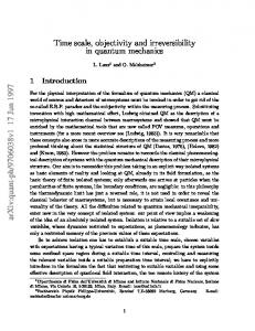
RETURN MAPS AND TIME IRREVERSIBILITY Time irreversibility is defined such that a qualitative or quantitative description of a time series and its time-reversed realization differ significantly. Time return maps provide a simple way to determine qualitatively whether engine data exhibit time irreversibility. Return maps plot each successive pair of timeseries values (i.e., the heat releases for every cycle i and cycle i + 1, where i is indexed from 1 to N ; 1 for a time series of N records) as points in a plane. With each new cycle, the current point “maps” into the next, building up a composite statistical picture of how cycles are interrelated. In return maps, timereversible data exhibit symmetry about the abscissa-ordinate equality diagonal, so that forward-time and reverse-time versions of the map appear similar. Time-irreversible data exhibit significant bias and asymmetry about the diagonal. Gaussian random data are time reversible and concentrate in a “fuzzy” circular region centered on the diagonal. Static transforms of Gaussian data warp the shape of the circular region but still exhibit symmetry about the diagonal. All experimental heatrelease data were verified to be statistically stationary, which excludes the possibility of observing time irreversibility in the data, or warping of the return maps, because of nonstationarity. Figure 1 illustrates this with return maps of cycle-resolved heat-release data from the four engines at three equivalence ratios. At stoichiometric fueling (K1, Q1, C1, and V1), cycle-to-cycle combustion dynamics appear stochastic in nature and Gaussian in distribution; the return maps appear as timereversible, fuzzy circular regions, and the range of heat-release variability is relatively small. As fueling is leaned (K2, Q2, C2, and V2), the onset of engine instability produces occasional misfires that create large excursions away from the central region on the return map. These partial-combustion heat releases appear as “arms” on the return maps. The excursions become larger as the engine is operated at very lean fueling (K3, Q3, C3, and V3), and the characteristic arms become denser. Complete misfires appear as flat regions near the ends of the arms (K3, Q3 and C3). The return maps exhibit increased asymmetry about the diagonal, and hence time irreversibility, as fueling is leaned. Particular asymmetric features to note are the second vertical band of points to the right of the diagonal (K2, K3, Q2 and C2) and the displacement of the “vertex” of the arms to the right of the diagonal (K3, Q3 and C3). In the following sections, we describe methods to quantify time irreversibility and to use this feature to compare the relative agreement between the the two classes of cyclic-variability models and our experimental heat-release data.
Heat release for cycle i
Heat release for cycle i
Heat release for cycle i
Heat release for cycle i+1
Heat release for cycle i
Heat release for cycle i
(C3) CFR at φ = 0.69 Heat release for cycle i+1
(C2) CFR at φ = 0.72 Heat release for cycle i+1
Heat release for cycle i (V2) V8 at φ = 0.71 Heat release for cycle i+1
(V1) V8 at φ = 1.00
Heat release for cycle i (V3) V8 at φ = 0.59 Heat release for cycle i+1
Heat release for cycle i+1
(Q3) Quad4 at φ = 0.73
Heat release for cycle i
(C1) CFR at φ = 1.00
Heat release for cycle i+1
Heat release for cycle i
(Q2) Quad4 at φ = 0.84 Heat release for cycle i+1
Heat release for cycle i+1
(Q1) Quad4 at φ = 0.99
Heat release for cycle i
(K3) Kohler at φ = 0.73 Heat release for cycle i+1
(K2) Kohler at φ = 0.77 Heat release for cycle i+1
Heat release for cycle i+1
(K1) Kohler at φ = 0.99
Heat release for cycle i
Heat release for cycle i
Figure 1: Time return maps for the four engines at three equivalence ratios for approximately 3000 contiguous engine cycles. The diagonal described in the text is plotted with the broken line (- - - -).
For quantitative evaluations of time irreversibility in engine heat-release measurements, we employ an approach known as symbolic time-series analysis, or symbolization for short. The symbolization methods we describe here are based on the general approach suggested by Tang et al. [9] with some modifications to address time irreversibility. For more detailed information on the theoretical basis and development of symbolization as a data-analysis tool, the reader is referred to Finney et al. [10] and Daw et al. [11]. The key step in symbolizing time-series measurements involves transforming the original values into a stream of discretized symbols. This discretization is accomplished by partitioning the range of the data values into a finite number of regions (usually less than 10) and then assigning a symbol to each measurement based on which region into which it falls. For example, the simplest scheme is to assign symbolic values of 0 or 1 to each observation depending on whether it is above or below some critical value. For the results presented here, we define our partitions such that the individual occurrence of each symbol is equiprobable (i.e., the likelihood of observing a single measurement in any given region is the same). Time series
Symbol
1
0
0 1 1 0 1 1 0 0 0 1 1 1 0 0 1 1 0 1 0 0 Symbol series
Figure 2: Example of data symbolization. Time-series points ( ) are discretized into symbols (0 or 1) based on values relative to the partition (- - - -). The solid curve (——) is for visualization only and should not imply a smooth dynamical flow between successive records in discrete time series such as cycle-resolved heat release. See text for explanation of bold points and symbols.
A simple illustration of data symbolization is shown in Fig. 2 for an artificial time series of 20 records. Data points (circles) below the partition (broken line) are assigned a symbolic value of 0, and points above the partion are symbolized as 1. The partition is defined such that the resulting symbol series has an equal number of 0s and 1s. Once a time series is symbolized, the relative frequencies of all possible sequences of consecutive symbols over a finite interval provide an efficient measure of temporal patterns in the data. A simple way to summarize the relative frequencies of each possible symbol sequence is to assign a unique number that identifies each sequence, thus making it possible to plot frequency versus sequence number in a plot called a symbolsequence histogram. We assign a sequence code to each pattern by using the decimal equivalent of each base-n sequence of length L, where n is the number of symbols. For exam-
ple, a symbol sequence of 1 0 1 (depicted in bold in Fig. 2), with n = 2 and L = 3, has a sequence code of 5, from 1 � 22 + 0 � 21 + 1 � 20 . Because of our equiprobable partitioning convention, the relative frequency of each sequence for random data will be equal (subject to sampling fluctuations). Thus any significant deviation from equiprobable sequences is indicative of time correlation and determinism.
4/18
Frequency
DATA SYMBOLIZATION
3/18 2/18 1/18 0/18
Sequence code 0 1 2 3 4 5 6 7 Sequence 000 001 010 011 100 101 110 111
Figure 3: Example symbol-sequence histogram for the time series depicted in Fig. 2. As seen in the histogram, the sequence 1 0 1 occurs two times in the symbol series, denoted in bold in Fig. 2. A simple illustration of a symbol-sequence histogram is shown in Fig. 3, created from the example time series of Fig. 2. Sequence 1 0 1 with sequence code 5 occurs two times in the symbol series (shown in bold in the figures). The sequence frequencies are normalized by 18 instead of 20 because there are only N ; L + 1 or 20 ; 3 + 1 possible sequences in the short example symbol series. Symbol-sequence histograms are useful for quantifying time irreversibility because the relative frequencies of certain symbol sequences will shift when the data are observed in reverse time. Conversely, for time-reversible data series, there should be no significant difference in the histogram whether it is constructed in forward or reverse time. To compare forwardand reverse-time histograms, we use a Euclidean-norm statistic defined by Tirr
=
sX i
(F
i ; Ri )2
(4)
where i is indexed over all possible sequence codes. F and R are the symbol-sequence histograms for the forward- and reverse-time analyses, respectively. The magnitude of T irr indicates the difference between the two histograms and thus quantifies the level of time irreversibility. Figure 4 illustrates symbol-sequence histograms for the forward- and reverse-time realizations of data from the four engines at three equivalence ratios. The reverse-time realization of each data set was produced by reversing the order of the time series. Each plot is in the same position as its corresponding return map in Fig. 1. The symbol-sequence histograms were produced using n = 8 symbols and a sequence length of L = 2 cycles. With this symbolization, there are nL = 82 = 64 possible sequences. Reported on each plot is the Tirr difference between the forward- and reverse-time symbol-sequence histograms. The plots in Fig. 4 provide both a visual and quantitative summary of the trends seen with the return maps in Fig. 1. At stoichiometric fueling (K1, Q1, C1, and V1), cycle-to-cycle
(K1) Kohler at φ = 0.99
(K2) Kohler at φ = 0.77
Tirr = 0.0210 0.06 0.04
0.1
0.08 Tirr = 0.0250 0.06 0.04 0.02
0 10
20 30 40 50 Sequence code
60
(Q1) Quad4 at φ = 0.99
20 30 40 50 Sequence code
60
0
Tirr = 0.0208 0.06 0.04 0.02
0.08 Tirr = 0.0295 0.06 0.04
(C1) CFR at φ = 1.00
10
20 30 40 50 Sequence code
0
0.06 0.04 0.02
0.08 Tirr = 0.0542 0.06 0.04
(V1) V8 at φ = 1.00
10
20 30 40 50 Sequence code
0
0.06 0.04 0.02
0.08 Tirr = 0.0341 0.06 0.04
60
0.08 Tirr = 0.0843 0.06 0.04 0.02
0 60
20 30 40 50 Sequence code
(V3) V8 at φ = 0.59
0.02
0
10
0.1
Relative frequency
Relative frequency
Tirr = 0.0203
20 30 40 50 Sequence code
0.04
(V2) V8 at φ = 0.71
0.08
10
Tirr = 0.0943 0.06
60
0.1
0
0.08
0 0
0.1
60
0.02
0 60
20 30 40 50 Sequence code
(C3) CFR at φ = 0.69
0.02
0
10
0.1
Relative frequency
Relative frequency
Tirr = 0.0167
20 30 40 50 Sequence code
0.04
(C2) CFR at φ = 0.72
0.08
10
Tirr = 0.0881 0.06
60
0.1
0
0.08
0 0
0.1
60
0.02
0 60
20 30 40 50 Sequence code
(Q3) Quad4 at φ = 0.73
0.02
0
10
0.1
Relative frequency
0.08
20 30 40 50 Sequence code
0.04
(Q2) Quad4 at φ = 0.84
Relative frequency
Relative frequency
10
0.1
10
Tirr = 0.1261 0.06
0 0
0.1
0
0.08
0.02
0 0
Relative frequency
Relative frequency
0.08
0.02
Relative frequency
(K3) Kohler at φ = 0.73
0.1
Relative frequency
Relative frequency
0.1
0 0
10
20 30 40 50 Sequence code
60
0
10
20 30 40 50 Sequence code
60
Figure 4: Symbol-sequence histograms for the four engines at three equivalence ratios for approximately 3000 contiguous engine cycles. Forward-time histograms are plotted with solid lines (——), reverse-time histograms with broken lines (- - - -).
combustion dynamics appear time-reversible in nature; there are only minor differences between the forward- and reversetime histograms. As fueling is leaned (K2, Q2, C2, and V2), clear differences are seen, particularly in C2 and V2, and the Tirr values rise accordingly. At very lean fueling (K3, Q3, C3, and V3), the combustion dynamics are highly time irreversible, evidenced by the striking visual differences in the histograms and their elevated Tirr differences. Physically, as fueling is leaned to the point in K3, Q3, C3, and V3, the combustion dynamics in the forward sense are dominated by sequence 0 7, yet the time-reverse sequence 7 0 is significantly less frequent. This sequence represents the occurrence of a partial burn or misfire followed by an energetic burn. The large difference in frequencies of 0 7 compared with 7 0 shows that there is a strong preference for the order in which they occur. As we describe in the next section, this preference for order has important implications for selecting the best model of cyclic variation. It should be noted that the deterministic rule used by Martin et al. [3] captured this prior-cycle effect. In their model, the IMEP of a cycle immediately following a very poor combustion cycle, defined by a threshold, was set to a relatively large value. MODEL DISCRIMINATION As previously discussed, two prominent explanations for cyclic variations are the LGRP and the NND classes of models. LGRP models are based on the hypothesis that cyclic variability occurs because of noisy, linear perturbations to the combustion process. Such perturbations could be caused by excited acoustic modes in the intake manifold. Because combustion efficiency is nonlinearly affected by small fluctuations in equivalence ratio near the lean limit (see [4] for a discussion of the combustionefficiency function), the as-injected fluctuations would tend to be amplified to produce large combustion variations. Since these fluctuations would be dominated by intake effects, the engine would simply follow the linear dynamics of the intake system. As a result, there is no nonlinear “memory” of past combustion events passed to the future. Therefore, the resulting combustion behavior would exhibit the noisy anticorrelated oscillations (alternating stronger and weaker heat-release values) observed in experimental data at lean fueling conditions. NND models assume that prior combustion events affect successive combustion events through some mechanism, such as residual gas. For example, residual fuel and air from past combustion events can mix with freshly injected fuel and air, causing wide variations in combustion. Unlike LGRP models, this type of nonlinear “memory” can produce much more interesting and complex behavior, most notably time irreversibility, bifurcations, and chaos. We constructed surrogate data sets from both LGRP and NND models to compare with our experimental data. To represent LGRP models, we used three approaches: an ARMA model, the model of Daw et al. [4] with residual effects disabled and driven with linearly filtered anticorrelated noise, and a data-transformation technique of Schreiber and Schmitz [12]. To simulate the ARMA model, we fit the experimental data using a second-order model and then generated surrogate data by driving the model with Gaussian noise. We used a program provided publicly by A. Schmitz [13] to generate the Schreiber-
Schmitz surrogates; the surrogate data produced with this program have the same autocorrelation and data-distribution characteristics as the experimental data, which we verified independently to assure that the program was working. To represent an NND model, we used an implementation of the model described in Daw et al. [4]. We illustrate examples using data from the V8 engine at an equivalence ratio of 0.59 (Fig. 1(V3)). We generated model data sets of approximately 3000 cycles each to simulate this experimental condition. The ARMA surrogates and the SchreiberSchmitz surrogates are both statistically based models, and the LGRP and NND surrogates of Daw et al. are physically based models with parameters set to approximate the conditions of the experimental data. Figure 5 shows return maps for the experimental and model data, and Fig. 6 shows the corresponding symbolsequence histograms using the same symbolization parameters as in Fig. 4. As seen in Fig. 5, both the transformed LGRP models and the NND model reproduce certain features observed experimentally at lean fueling. For example, the global patterns have a characteristic “crescent” shape opening to the left. However, on careful examination, we see that the NND return map exhibits a definite asymmetry about the diagonal, while the LGRP return maps appear at least qualitatively symmetric. The ARMA model return map appears ellipsoidal and symmetric about the diagonal but does not reproduce the qualitative shape of the experimental data. In the symbol-sequence histograms comparing both forward- and reverse-time realizations of each data set (Fig. 6), only the NND model reproduces the same qualitative time irreversibility as the experimental data, and its Tirr difference is more similar to that of the experimental data than those of the other models. These trends are reproducible over a range of lean fueling conditions and suggest that models which cannot reproduce the time irreversibility observed in experimental data insufficiently describe the combustion dynamics. The NND model captures this time-irreversibility feature but may be inaccurate and unrealistic in other respects (e.g., effects of diluents and temperature on flame speed and combustion efficiency).
SUMMARY Experimental data from four different engines exhibit pronounced time irreversibility in cycle-to-cycle combustion variations under lean fueling conditions. The occurrence of significant time irreversibility automatically excludes LGRP models as candidates for describing combustion variability. On the other hand, NND models readily reproduce the observed irreversibilities. Data symbolization appears to be a very effective method for detecting and quantifying irreversibility.
ACKNOWLEDGEMENTS The authors thank F.T. Connolly of the Ford Motor Company for providing experimental data from the V8 engine.
Heat release for cycle i+1
V8 at φ = 0.59
Heat release for cycle i+1
LGRP model of Daw et al.
Heat release for cycle i+1
ARMA surrogate
Heat release for cycle i
Heat release for cycle i
Heat release for cycle i
Heat release for cycle i+1
NND model of Daw et al.
Heat release for cycle i+1
Schreiber-Schmitz surrogate
Heat release for cycle i
Heat release for cycle i
Figure 5: Time return maps for the V8 engine data at equivalence ratio of 0.59 (Fig. 1(V3)) and four model data sets for approximately 3000 contiguous engine cycles.
ARMA surrogate
LGRP model of Daw et al.
V8 at φ = 0.59
0.08 Tirr = 0.0200 0.06 0.04 0.02
0.08
0
Tirr = 0.0843
Tirr = 0.0205 0.06 0.04
0 0
0.06
0.08
0.02
0.04
10
20 30 40 50 Sequence code
60
0
Schreiber-Schmitz surrogate
0 0
10
20 30 40 50 Sequence code
60
Relative frequency
0.02
10
20 30 40 50 Sequence code
60
NND model of Daw et al.
0.1
0.1
Relative frequency
Relative frequency
0.1
0.1
Relative frequency
Relative frequency
0.1
0.08 Tirr = 0.0173 0.06 0.04 0.02
0.08 Tirr = 0.0910 0.06 0.04 0.02
0
0 0
10
20 30 40 50 Sequence code
60
0
10
20 30 40 50 Sequence code
60
Figure 6: Symbol-sequence histograms for the V8 engine data at equivalence ratio of 0.59 (Fig. 1(V3)) and four model data sets for approximately 3000 contiguous engine cycles. Forward-time histograms are plotted with solid lines (——), reverse-time histograms with broken lines (- - - -).
REFERENCES
NOMENCLATURE
[1] Belmont M.R., Hancock M.S., Buckingham D.J. (1986). “Statistical aspects of cyclic variability”, SAE Paper No. 860324.
L
[2] Scholl D. (Ford Motor Company) (1997). Electronic-mail message to C.S. Daw (Oak Ridge National Laboratory), 1997 October 22.
Tirr
[3] Martin J.K., Plee S.L., Remboski D.J. Jr. (1988). “Burn modes and prior-cycle effects on cyclic variations in leanburn spark-ignition engine combustion”, SAE Paper No. 880201. [4] Daw C.S., Finney C.E.A., Green J.B. Jr., Kennel M.B., Thomas J.F., Connolly F.T. (1996). “A simple model for cyclic variations in a spark-ignition engine”, SAE Paper No. 962086.
N n
Number of consecutive symbols in a symbol sequence Number of records in a time series Number of symbols used to transform a time series into a symbol series Euclidean norm between the forward- and reversetime symbol-sequence histograms
ABBREVIATIONS ARMA CV EGR IMEP LGRP NND RPM SI
[5] Diks C., Houwelingen J.C. van, Takens F., DeGoede J. (1995). “Reversibility as a criterion for discriminating time series”, Physics Letters A 201, 221–228. [6] Weiss G. (1975). “Time-reversibility of linear stochastic processes”, Journal of Applied Probability 12, 831–836. [7] Grimm B.M., Johnson R.T. (1990). “Review of simple heat release computations”, SAE Paper No. 900445. [8] Heywood J.B. (1988). Internal Combustion Engine Fundamentals, McGraw-Hill, ISBN 0-07-028637-X. [9] Tang X.Z., Tracy E.R., Boozer A.D., deBrauw A., Brown R. (1995). “Symbol sequence statistics in noisy chaotic signal reconstruction”, Physical Review E 51:5, 3871– 3889. [10] Finney C.E.A., Green J.B. Jr., Daw C.S. (1998). “Symbolic time-series analysis of engine combustion measurements”, SAE Paper No. 980624. [11] Daw C.S., Kennel M.B., Finney C.E.A., Connolly F.T. (1998). “Observing and modeling nonlinear dynamics in an internal combustion engine”, Physical Review E 57:3, 2811–2819. [12] Schreiber T., Schmitz A. (1996). “Improved surrogate data for nonlinearity tests”, Physical Review Letters 77, 635– 638. [13] Schmitz A. (1997). C-language computer program surrogates. The TISEAN software package is publicly available at either http://www.mpipks-dresden.mpg.de/˜tsa/TISEAN/docs/welcome.html or http://wptu38.physik.uni-wuppertal.de/Chaos/DOCS/welcome.html.
Autoregressive moving average Cyclic variability Exhaust-gas recirculation Indicated mean effective pressure Linear Gaussian random process Noisy nonlinear dynamics Revolutions per minute Spark ignited