Time-Optimal Network Queue Control : The Case of a Single Congested Node Mahadevan Iyer
Wei Kang Tsai
Dept. of Electrical and Computer Engg. University of California, Irvine Irvine, USA
[email protected]
Dept. of Electrical and Computer Engg. University of California, Irvine Irvine, USA
[email protected]
Abstract---We solve the problem of time-optimal network queue control: what are the input data rates that make network queue sizes converge to their ideal size in the least possible time after a disturbance while still maintaining maximum link utilization at all times, even in the transient? The problem is non-trivial especially because of the vast possible heterogeneity in packet propagation delays in the network. In this paper, we derive the time-optimal queue control for a single congested network node with a single finite queue shared by flows with arbitrary network delays. We neatly separate the derivation of the optimal arrival rate sequence from that of the feedback control protocol to achieve it. The time-optimal control is robust to bandwidth and queue size estimation errors. Its complexity is only a function of the size of the network delays and no per-flow computation is needed. The time-optimality and robustness properties are proven to hold under all queue operating regimes with no need for linearizing approximations. Keywords--- Flow Control, Queue Control, Congestion Control, Control Theory, Optimization, ATM, ABR
I. INTRODUCTION Networks all over the world, both public and private, are facing continuously increasing traffic loads. In recent developments, the long touted convergence of traditional telephone services to the Internet is finally happening slowly but surely. VoIP (Voice over IP) traffic has seen a gradual increase over the last two years, especially in private intranets as enterprises realize its cost and flexibility benefits. Peer-toPeer data traffic is on the rise and has to be controlled so as to protect other data applications. Broadband wireless LAN traffic is on a steep rise and is expected to contribute significantly to backbone networks of service providers. High bandwidth video traffic will also undergo a steep rise once broadband to the home becomes ubiquitous. With such bandwidth-hungry traffic on the rise and additional raw bandwidth still being costly to deploy, the problem of coordinated network-wide congestion prevention and queue control will assume paramount importance more than ever. The disturbances in the available bandwidth for any class of traffic will become more severe. Users will establish or break flows on a larger scale. Higher priority traffic classes may suddenly consume or release large amounts of
0-7803-7753-2/03/$17.00 (C) 2003 IEEE
bandwidth. These can lead to sudden and large changes in queue sizes and link utilization. In the light of this reality, this paper seeks to answer a fundamental question: how should the flow source rates feeding into a network be adjusted so as to quickly bring the network back towards its ideal steady queue-size condition after a disturbance. In fact, how fast can this be done while always ensuring full utilization at some link in the path of every traffic flow? How does the per-flow service rate allocation used at the queues affect this convergence time? What makes this particular control problem uniquely challenging is the presence of time delays in the data and control feedback paths. We believe that the solution to this time-delayed control problem is important in the design of any practical flow control scheme that has to handle large disturbances. More formally, the general time-optimal queue control problem is: given initial queue sizes, and the link bandwidths for all future times, determine the source rate sequences and the per-flow service rates at queues that will bring the queue sizes to desired values in minimum time, while ensuring that at least one link remains fully utilized in every flow’s path. We seek solutions to this problem with a gradual approach. In this paper, we solve this problem for the case of a single congested node in the network, with the flows sharing a single queue and being jointly controlled. In a subsequent paper we generalize the solution for the case of multiple congested nodes. As we see later in this paper, a sufficient condition for convergence (after a disturbance) to ideal queue sizes in minimum time is basically the minimization of magnitude of a queue deviation term at every point in time. This queue deviation term is the current queue size minus the ideal queue size reduced by an overload term. This overload is the total future queue size increase contributed by erroneously computed past rates that did not anticipate the disturbance. This has never been explicitly and precisely taken into account in previous approaches to flow control and the emphasis on time-optimal control is what led to its discovery. Unlike past control theoretic approaches, including those based on linear-quadratic optimal control [1,2,5], we neatly separate the derivation of the optimal arrival rate schedules from the closed-loop network protocol to achieve it. Other
IEEE INFOCOM 2003
than fastest convergence, the other noteworthy features of the time-optimal control and its corresponding protocol are: 1. Global Stability: Queue size convergence in minimum time is guaranteed under all initial conditions and initial traffic disturbances even if queue operation enters the nonlinear regime. 2. Tight Robustness of Performance: The deviations of the queue sizes from their time-optimal values are bounded by exactly the total error bound in estimating the queue size and available link capacity terms in the control. Intuitively, this will also imply robustness of the timeoptimal protocol to link delay estimation errors since these contribute bounded errors in estimating the future queue size and capacity terms in the control. 3. Simplicity: The structure of the time-optimal control is simple: a residual-capacity term minus a queue deviation term. 4. Scalability: The control rates need to be computed only per flow delay and not per flow. If D is the maximum round-trip time in units of discrete control intervals, the control complexity is O ( D 2 ) at the time of a disturbance and O(W) otherwise, where W ≤ D is the number of different flow fairness weights. 5. Fairness: Once the expression for the time-optimal total arrival rate is calculated, it can be divided in any desired proportion to obtain the individual flow rates to be fed back from switch to each flow source. In practice, time-optimality in control becomes most important during periods of large queue deviations, while slower control can be used during other periods [14].
Related Work Numerous network flow control schemes have been proposed. The schemes surveyed in [12] and those in [7,8,14] have focused primarily on the fairness to different flows and maximal utilization of available link capacity while using adhoc enhancements for queue control. Recently, linear controltheory has been systematically applied to control of TCP flows using active queue management ([9]) in Internet routers in [10] which also contains references to numerous other TCP control-theoretic analyses. However in this paper, we focus on more closely related work on network level rate-based feedback flow control using control theory. [3] presented one of the first network-layer flow control schemes to systematically apply linear feedback control theory. The scheme controls a single congested queue in a provably local-asymptotically stable manner, with arbitrary but fixed network delays. Local stability here means guaranteed queue convergence after a small initial disturbance in available link capacity or set of flows. The disturbance is assumed small enough to ensure linear operation i.e. full link utilization and no buffer overflow at all times, even in the initial round-trip time following a disturbance. [4] extends [3] to multiple congested nodes. In [3,4], the available capacity changes are kept track of indirectly by tracking changes in
0-7803-7753-2/03/$17.00 (C) 2003 IEEE
queue size. This indirect and moreover linear control approach for a nonlinear system like a network queue makes it very difficult to ensure global stability. [16,17] use the classical Smith predictor approach [21] to ensure local asymptotic stability in the presence of network delays. [18] improves on [17] by using a robust decoupled queue-reference and ratereference control that needs no direct knowledge of network delays. [16-18] are all per-flow control schemes and do not consider the idea of joint optimal control of all flows. The linear controller in [15], like [3], does not use the available capacity term directly but only by tracking the current change in queue size. But it is a dual controller: after a disturbance, a high gain controller quickly brings the queue to near the equilibrium point after which a low gain controller takes over and maintains local stability around the equilibrium point. [5] presents a linear-quadratic optimal control approach for per-flow control. Recent papers [1,2] formulate singlequeue control as a stochastic optimal control problem with heterogeneous network delays. However [1,2] also assume a linear operation for the queue at all times. [6] derives stochastic optimal control policies assuming Markovmodulated capacity variations. [20] designs robust controllers to handle uncertain and heterogeneous network delays, but assumes linear operation too. The rest of the paper is organized as follows. Section 2 informally explains time-optimal control. Section 3 mathematically formulates the time-optimal control problem. Section 4 derives the time-optimal input rates first for a single flow and then generalizes to multiple flows. Section 5 derives a switch-centric feedback protocol to achieve the time-optimal control. Section 6 proves the robustness of the time-optimal control. Section 7 makes concluding remarks. II. INFORMAL DISCUSSION OF TIME-OPTIMAL QUEUE CONTROL
Consider first the simple one queue/link model of Fig. 1. The queue size Q(n) and output data rate o(n) get updated regularly according to the discrete-time update equation1, Q ( n + 1) = (Q (n ) + a ( n ) − C ( n )) + (1) (2) o( n ) = min(Q (n ) + a ( n ), C (n ))
where x + = max( x,0) , a(n) is the data arrival rate and C(n) is the available link capacity (or service rate) of the queue in the th n time-slot, both measured in bits per time slot. In words, if the demand (total arrival rate plus queue size) is no greater than the link capacity in a time slot, the queue goes to zero; otherwise the excess of demand over capacity remains in the queue. The network node buffer holding the queue is assumed infinite for now. Finite buffers are considered in section 4.
1
In the rest of the paper, an expression of the form x + will stand for max( x,0) and x − for min( x,0) .
IEEE INFOCOM 2003
Q(n)
a(n)
Q*
Control Phase 1
Time of Disturbance
o(n)
C(n)
n
Switch
...
Control Phase 2
. . .
n+D1
n+D2
n+D 3
.
n+D N
...
Flow 1
Fig. 1. Quantities involved in single queue control.
...
Flow 2
Flow 3
Supposing our ideal state is one of zero queue size and full link utilization. A trivial way to reach this state as quickly as possible is simply not transmit any data into the queue until the initial Q(0) bits of data are completely drained out and after that keep the data arrival rate equal to the available capacity at all times. The trouble with this approach is that the link can remain underutilized when Q(n) < C(n) and no data is sent; the entire queue would drain out and yet not utilize all the available link capacity. Indeed, a careful look at the queue update equations above shows that only when the queue size is larger than the available link capacity must the arrival rate must be 0 to achieve maximum queue drainage in that time slot. However, when the queue size is smaller than available capacity, the ‘room’ available in the queue is the available link capacity minus the queue size, C ( n ) − Q ( n ) , and an arrival rate of this value will send the queue to zero at the end of that time slot while still fully utilizing the link, i.e. o(n ) = C ( n ) . Hence the
. . .
Control Information Trajectory
Data Trajectory
Time
Flow N
Fig. 2. Control Phases and Data Trajectories desired arrival rate information being conveyed by the switch to each flow source which then respond with data traveling along the trajectories shown by the forward slanted lines. The time-axis gets divided into control phases with phase i being from n = Di to n = Di +1 where Di is the round-trip time for the ith nearest source. In other words, the control phase in which a time slot n resides is P(n) where P(n) = i if Di ≤ n < Di +1 Thus during phase 0, all flows are sending pre-disturbance rates, during phase 1, only flow one is sending the newly controlled (post-disturbance) rates, during phase 2, flows 1 and 2 are sending newly controlled rates and so on. In general, the controllable flows at time n are from i=1 to P( n ) or
arrival rate must be controlled as a* (n ) = (C (n ) − Q (n )) + in order to minimize the queue size and maximize the link utilization at every time step. Minimizing the queue size at every time step in turn minimizes the time to converge the queue size to zero. In general if the target queue size is Q * , it’s the magnitude equivalently all i such that n ≥ Di . The queue update of queue size deviation, q(n ) = Q ( n ) − Q * , and not the queue equation can be then written purely in terms of the total arrival size that must be minimized at every time step. The time- rate of these controllable flows and the capacity available to them. That is, optimal arrival rate must therefore be, a* (n ) = (C ( n ) − q(n )) + (3) Section 4 formally proves that (3) is indeed time-optimal, i.e. converges q(n ) to zero in minimum time and fully uses the link capacity at all times. The time-optimal source rates are then merely a time-delayed version of the time-optimal arrival rates. Next, consider multiple flows sending data into the same queue. The flow sources are located at different distances from the queue as for example in Fig. 3. Consider a disturbance in the future capacities, as estimated by an observer at the queue. Upon detecting such a disturbance, it takes one round-trip time for the new desired arrival rate to be conveyed back to a source and the data from the source to be arriving later at the queue at this new rate. This is illustrated in fig. 2. The x-axis is the time and the y-axis is the distance away from the switch towards the various sources. The backward slanted line shows
0-7803-7753-2/03/$17.00 (C) 2003 IEEE
N
Q ( n + 1) = (Q ( n ) +
∑ a (n) − C (n)) i
+
i =1
= (Q (n ) + a c (n ) − C c (n )) +
where a c (n ) =
∑ a (n )
(4) (5)
i
i:n ≥ Di
is the total controllable arrival rate and C c ( n ) = C (n ) −
∑ a (n) i
(6)
i:n < Di
is the controllable capacity. But this queue update equation is exactly that of a single flow through a single queue as in (1). The single flow is really a super-flow, an aggregate of the controllable flows identified for each give time slot.
IEEE INFOCOM 2003
C c (m) 0 D1
Flow 1 D1=3 ms
n
S(n)
D2
m
Q * Q ( n ) Q e* (n ) C ( n)
D2=10 ms
Flow 2
S (n)
Fig. 3. Illustration of time-optimal control with negative controllable link capacity However there is one crucial difference between equations (1) and (4). Unlike C ( n ) , C c ( n ) can go negative when the longer uncontrollable flows are sending more than the available link capacity, something that occurs significantly in practice due to sudden available capacity drops or new flows joining, say due to route changes. Hence the control given by (3) has to be generalized to handle negative capacities. Intuitively, an extra space must be reserved in the queue to accommodate the queue buildups represented by the negative capacities in the future. That means the target queue size value must be effectively reduced by the sum of the future negative capacities. Fig. 3 shows an example. Two flows cross a queue. Flow 1 has shorter round-trip delay of 3 ms and flow 2 has a round-trip delay of 10 ms. The target queue size is 50 Kb and at any time n in control phase 1, the total future negative capacity seen by flow 1, as represented by the shaded area in the figure, is -30 Kb. This is the total data going to be dumped in the queue by flow 2 in control phase 1 even if nothing arrives from flow 1. Hence a queue space of 30 Kb must be ‘reserved’ for these and the effective target queue size is 50– 30=20 Kb. In general, the effective target queue size at time n is Q e* = (Q* + S ( n )) + where S (n ) =
∑ (C (l )) c
−
l ≥n
is the total negative controllable capacity in the future of n. We also call S (n ) as the future overload at time n. The arrival rates must therefore be calculated as a c* ( n ) = (C c ( n ) − qe (n )) + (7) where qe (n ) = Q ( n ) − Q e* (8) In the following section, we formally define the time-optimal control problem within a reasonably simplified network model. Section 4 then formally proves that (7,8) is indeed the solution to the time-optimal control problem: it achieves minimum convergence time while ensuring full link utilization at all times.
0-7803-7753-2/03/$17.00 (C) 2003 IEEE
III. NETWORK MODEL AND THE TIME-OPTIMAL CONTROL PROBLEM
A. Network Model Since the objective of this paper is to gain a fundamental understanding of time-optimal queue control, we keep the network model simple and make some reasonable simplifying assumptions. The network is modeled as a set of packetswitched nodes interconnected by links. A flow is a stream of packets traveling from a given source to a destination through a fixed sequence of links and nodes. This models even a datagram network reasonably well for the purpose of feedback flow control, provided the datagram routes change only on the order of several round trip times, e.g. IP networks [18]. The source and destination nodes could either be end hosts or edge nodes of the network. The set of packets that have entered a node and are waiting to be routed on to a particular link are represented by a queue to that link. This model is general enough to represent any combination of input or output queuing done in present day routers. All the flow control is concerned with is the size of this queue and not with the particular queuing implementation used inside the node/router. In this paper, we only consider the control of a single queue in a single bottleneck node in the network. The total access link delay between transmission of a packet at a source and its reception at the bottleneck node queue can be assumed fixed since no variable queuing delays will be encountered by the packet until it reaches the bottleneck queue. This is a simplified model and also a first step in tackling the more general problem of multiple queues with arbitrary network topology and flow routes [11]. Time is divided into a sequence of time slots and all control computations are done at the beginning of time slots. Different packets can be of different sizes, with all traffic rates measured in number of bits per time slot. The input rate in a given time slot is the number of bits that enter the queue in that time slot while the available link capacity in a time slot is the maximum number of bits that can be served from the queue in that time slot. This available link capacity value is something determined by the local capacity allocation scheme used inside the node. For example, in the ATM ABR or IP best effort service, it is basically the total outgoing link capacity minus that consumed by the higher priority VBR or DiffServ flows. All the access link delays in this paper are assumed to be and expressed in integer number of time slots. Non-integer delays can be handled in a manner similar to that in [3]. Buffer Size Assumption: Initially, we assume the buffer holding the data queue to be infinite in size. At the end of section 4, we explain why the time-optimal control law of (7), (8) still holds for any buffer size, finite or infinite.
IEEE INFOCOM 2003
Delay-Based Aggregation of Individual Flows: All individual flows with equal round-trip delays, measured in units of time slots, are aggregated together as a single flow. In the rest of the paper, a “flow” refers to this aggregated flow. The flows are then identified by integers such that flow th number i has the i smallest round-trip delay.
C( n ) = {C (n ) : n ≥ 0} is the link capacity sequence. This notation Q (I, C, a, n) is needed to compare the queue sizes caused by the candidate time-optimal sequence and other sequences, in the subsequent proofs in this paper. The queue size deviation is then q (I, C, a, n) = Q (I, C, a, n) − Q*
Notations and Terminology: The total forward access link delay for data packets along the B. The Time-Optimal Queue Control Problem path of flow i from source up to the queue is denoted by d fi . The backward access link delay for the control packets from Definition (Convergence): The queue size is said to have converged to a value at a given the queue back to source i is denoted by dbi . The round trip time n if it remains at that value from n onwards. time is Di ≡ d fi + dbi . The arrival rate at queue for source i at time n is the number of bits of flow i arriving at the queue in Given initial condition I, the link capacity sequence C, and a time slot n and is denoted by ai (n) . The source rate of flow i vector of controllable arrival rate sequences a, the earliest time * at time n is the number of bits transmitted by source in time at which the queue size has converged to Q , is called the slot n and denoted by Ai (n) . Obviously, convergence time to Q * and is denoted by T (Q * , I, C, a) . ai (n ) = Ai (n − d fi ) The total arrival rate at time n is a (n ) ≡
c
(9)
∑ a (n) . i
The
i
available link capacity (or the service rate) for the queue in time slot n is the maximum number of bits that can be transmitted on the outgoing link during time slot n and is denoted by C(n). The queue size at time n is the number of bits in the queue at the beginning of time slot n and denoted by Q(n). The queue deviation at time n is defined as q(n ) ≡ Q ( n ) − Q * where Q * is the target queue size. The queue output rate in time slot n is the total number of bits transmitted to the outgoing link and denoted by o(n).
The Single Queue Time-Optimal Control Problem can now be succinctly defined: Given an initial condition and the available link capacity sequence, find the vector of controllable arrival rate sequences that minimizes the convergence time to Q * while fully utilizing the available link capacity in every time slot.
Some convenient terminology for comparing queue sizes caused by optimal and non-optimal arrival rate sequences: In the time-optimal control problem, the I and C are given and are therefore dropped from the notation. The queue at time n caused by arrival sequence a is therefore simply denoted by Q (a, n ) . Queue and Output Update Equations: As discussed at the beginning of section 2, we use a discrete To further simplify expressions in the proofs, time update model for the queue size and output rates, viz. a) the phrase “ Q (a* , n ) ≤ Q (a, n ) ∀a ” is replaced by (10) Q ( n + 1) = (Q (n ) + a ( n ) − C ( n )) + “ Q (a* , n ) is the minimum” where a* is the candidate (11) o( n ) = min(Q (n ) + a ( n ), C (n )) sequence whose time-optimality is being proven.
b) Q(a * , n) is abbreviated as Q(n) Initial Conditions for the Control: c) a) and b) above also apply for q(.) and |q(.)| instead of The initial conditions for the control are the initial queue Q(.). size, Q (0) = Q0 , and the given arrival rates for each flow in its uncontrollable phase, viz. the tuple, I = {Q (0) = Q0 ,{ai ( n ) : 0 ≤ n < Di }i } IV. SOLUTION TO THE TIME-OPTIMAL CONTROL PROBLEM
Full Notation for Queue Size Sequence: From the update equation, (10), it follows that the sequence of queue sizes is a deterministic function of the initial condition, arrival rate sequences in the controllable phase for each flow, and the link capacity sequence. In other words, the queue size sequence can be fully described by the notation Q(I, C, a, n) where a(n ) = {ai ( n ) : n ≥ Di }i is the vector of controllable arrival rate sequences and
0-7803-7753-2/03/$17.00 (C) 2003 IEEE
In section 2, we made an intuitive guess at the solution by first looking at control of only a single flow arriving at the queue and then extending the solution to the case of multiple flows. This extension was done by showing that the queue update equation with multiple flows is equivalent to that of a single “controllable” flow crossing a queue with possible negative outgoing link capacities. The original single-flow control was then extended to handle negative link capacities.
IEEE INFOCOM 2003
In this section, we provide formal proofs to that these solutions are correct. The technique is to first prove that to achieve minimum convergence time, it is sufficient to keep a certain queue deviation magnitude term minimized at every time slot. Then we prove by induction on the time slots that the candidate control we guessed at, indeed minimizes the queue deviation magnitude at every time step and also keeps the link fully utilized. A. Single-Flow Time-Optimal Control
Lemma 1 (Sufficient Condition for Minimum Convergence Time (C1)) Given initial conditions I and the capacity sequence C. Let a be an arrival rate sequence such that for all n ≥ 0 , | q (a , n)| is the minimum. Then a achieves minimum convergence time. Proof: Consider any arrival sequence a’. Let n ≥ Tc (a ') . Then | q (a , n)| ≤ | q (a ' , n)| = 0 . Hence Tc (a) ≤ Tc (a ') . Theorem 1 (Time-Optimal Arrival Rates)
The arrival rate sequence a* ( n ) = (C (n ) − q( n )) + solves the single-queue time-optimal control problem.
For proving full utilization of link bandwidth, it is sufficient to prove that the total demand is always greater than link capacity, i.e. a* ( n ) + Q (n ) ≥ C ( n ) . But this is always true because a * ( n ) + Q ( n ) ≥ C ( n ) − q( n ) + Q ( n ) ≥ C ( n ) + Q * B. Multiple-Flow Time-Optimal Control Lemma 2 below proves a sufficient condition similar to that Lemma 1, but for the case of possibly negative capacities. The difference is that the target queue size Q * is replaced by a reduced target queue size (Q * + S (n − 1)) + . This reduction by S(n-1) leaves room in the queue at the beginning of time slot n for the total negative capacity (the total data going to be dumped into the queue due to overload) in the future. Thus, the deviation whose magnitude is to be minimized at every point in time now becomes ) q (a, n ) = Q(a, n ) − (Q * + S ( n − 1)) + (12) ) We call q (a, n ) as the overload-aware queue deviation at time n.
Lemma 2 (Sufficient Condition for Minimum Convergence Time (S1)) Given initial conditions I and the capacity sequence C. Let a arrival rate sequences such that for Proof: We prove by induction on n that the following two be a vector of controllable ) all n ≥ 0 , | q (a, n ) | is the minimum. Then a achieves conditions hold true for all n: C1(n): | q(n ) | is the minimum. minimum convergence time. Proof: Consider any arrival rate sequence a′ . Let n ≥ Tc (a′) . C2(n): if q(n ) > 0 , then q(a, n ) > 0 ∀a . By Lemma 1, C1 will guarantee minimum convergence time. Then, C2 facilitates the proof by strengthening the induction step. q(a′, m ) = 0 ∀m ≥ n => 0 ≤ a '( m) = C ( m ) ∀m ≥ n Base Case: Since Q (a,0) = Q0 is a given initial condition in => S (m − 1) = 0 ∀m ≥ n the problem, C1(0) and C2(0) are satisfied trivially. From (12) this implies, ) ) | q(a, m) |=| q (a, m ) |≤| q (a ', m ) |=| q(a ', m ) |= 0 Induction Step: Let C1(n), C2(n) hold true. We have, => Tc ( A ) ≤ Tc ( A ' ) Q(n + 1) = (Q (n ) + (C ( n ) − q(n )) + − C (n )) + Theorem 2 below proves the time-optimality of the control Case 1: q(n ) ≤ C ( n ) . Then by the above equation we have given by (7,8). * Q ( n + 1) = Q and hence | q (n + 1)| = 0 and is the minimum. This satisfies both C1(n+1) and C2(n+1). Theorem 2 (Time-Optimal Arrival Rates) Any vector of controllable arrival rate sequences that satisfies Case 2: q(n ) > C ( n ) ≥ 0 . Therefore q (n) =| q (n)| and is also a c* ( n ) = (C c ( n ) − qe (n )) + where qe (n ) = Q ( n ) − Q e* and the minimum by the inductive assumptions C1(n) and C2(n). Q e* = (Q* + S ( n )) + solves the single-queue time-optimal Since a* ( n ) = 0 , we have from (10), control problem. q (n + 1) = q (n) − C (n) > 0 Proof: We prove by induction on n that the following two Hence, conditions hold true for all n: ) ∀a , q(a, n + 1) ≥ q(a, n ) − C ( n ) ≥ q( n ) − C ( n ) = q(n + 1) > 0 S1(n): | q ( n ) | is the minimum. ) ) S2(n): if q (n ) > 0 , then q (a, n ) > 0 ∀a . which satisfies both C1(n+1) and C2(n+1). By Lemma 2, S1 will guarantee minimum convergence time. S2 facilitates the proof by strengthening the induction step.
0-7803-7753-2/03/$17.00 (C) 2003 IEEE
IEEE INFOCOM 2003
The full-link-utilization property will be proven at the end. In this paper, we assume the ERs of the non-bottleneck The proof by induction is given in Appendix A. switches to be always larger than that of the bottleneck switch. Therefore a flow ER sent by the bottleneck switch to the Fairness: source is actuated one round-trip time later as a data arrival Once the optimal total controllable arrival rate sequence is rate. Thus, denoting the bottleneck switch ER fed back to found, it can be divided in any desired proportion in each time source i at time m by R i (m ) we have, slot among the individual controllable flows. In general, this ai (m ) = Ai ( m − d fi ) = R i (m − Di ) proportion itself varies from time slot to time slot. Denoting wi (n ) as the fraction of a c* (n ) that is given to controllable Substituting the above equation in (6), we have, C c ( m) = C ( m ) − R i ( m − Di ) flow i at time n, we have the general flow rate allocation as,
∑
i:m < Di
ai* (n ) = wi (n )a c* (n ) ∀n ≥ Di
Note that the (6) and the above equation hold for a control starting from time 0. The switch however re-predicts future wi ( n ) = 1 capacities and re-computes the control afresh at every the i≤P(n) beginning of every time slot in general. For a control to be reP(n), as we recall from section 2, is the total number of computed at time slot n, the above equation now has to be controllable flows at time n. The simplest fair allocation time-shifted by n and therefore becomes, scheme is wi ( n ) = 1/ P(n ) . In the most general case one could Cˆ c ( n, m ) = Cˆ (n, m ) − R i ( m − Di ) (13) vary wi (n ) with n in such a way as to ensure long term i:m < n + D weighted fairness on any required time-scale. where Cˆ ( n, m) is the switch’s prediction of C ( m) at time n.
where
∑
∑
i
Independence of Time-Optimal Control Law on Buffer Size: So far we have assumed an infinite buffer to be holding the queue of data in the network node. With a finite buffer of size B, the queue update equation (1) is modified to (A.1) Q ( n + 1) = min( B, (Q (n ) + a ( n ) − C ( n )) + ) Note that Q ( n + 1) is still a monotonically increasing function of Q ( n ) and a (n ) . Because of this, all inequality comparisons in the proof of Theorem 2 still hold true even after replacing (Q(n)+a(n)-C(n))+ with min(B, (Q(n)+a(n)C(n))+). Hence Theorem 2 is true even with a finite buffer. Other than through a technical examination of the proof steps, one can also guess the reason for this intuitively: the control of (7,8) always tries to converge the queue towards the effective target queue size and away from the buffer limit. In the next section, the switch algorithm will use the finite buffer equation (A.1) instead of (1) in order to predict the future queue sizes correctly.
Note that the summation term in (13) goes to zero for m ≥ n + DN . Hence Cˆ c ( n, m ) = Cˆ (n, m ) ≥ 0 for m ≥ n + DN (14) Because of (14), the predicted future overload for time m from negative controllable capacities becomes Sˆ (n, m ) =
n + DN −1
∑
(Cˆ c ( n, l )) −
(15)
l =m
We now develop the switch pseudo-code. At the beginning of every time slot, the future capacities are predicted by a separate procedure, predict_capacities(). Then in procedure compute_optimal_rates(), (13), (15), (8) and (7) are used in a co-iterative computation of the optimal input rates and future queue sizes from m=n to m= n + DN . The data variables Sˆ (m ) and Cˆ ( m) hold the computed values of Cˆ ( n, m) and Sˆ (n, m) at time n. The pseudocode for the computation at a switch is thus:
V. A SWITCH-SOURCE PROTOCOL TO ACHIEVE TIME-OPTIMAL CONTROL
main() { // n is current time // predict the future C (m) s for (m = n to n + D ) Cˆ ( m) = predict_capacities(m);
The control feedback framework we consider is a similar to that of the ATM-ABR service, but simpler. Control packets N regularly travel from the source through each node in its path compute_optimal_rates (n, n + DN ); upto the destination and then reverse their paths back to the } source. Explicit rates (ERs) are computed for each time slot Algorithm 1: Switch Control Algorithm for each flow by the switch in a node. On receiving a control packet from a downstream switch, the switch replaces the ER in that packet with the minimum of that ER and the locally where the procedure compute_optimal_rates() is as follows: computed ER for the current time slot. The source thus receives the minimum of the ERs of each switch in its flow path. The source then equates its transmission rate to the latest compute_time_optimal_rates( window_start, window_end ) { ER it has received.
0-7803-7753-2/03/$17.00 (C) 2003 IEEE
IEEE INFOCOM 2003
// B is the size of the buffer holding the queue of data // P(m) is the control phase in which m resides //compute the current and future controllable capacities first for (m = window_start to window_end) { if ( m < n + DN ) Cˆ c (m ) = Cˆ (m ) −
∑
Ri ( m − Di ) ;
i:m < n + Di
} //compute the overload terms using a backward recursion on time m Sˆ ( n + D ) ← 0 ; N
(L1) for (m = n + DN − 1 to n) Sˆ ( m) ← Sˆ ( m + 1) + (Cˆ c ( m + 1)) − ;
// compute one window full of optimal input rates into the future (L2) for (m = window_start to window_end) { // the controllable rates start only from n + D1 if ( m ≥ n + D1 ) { qˆ e ( m) ← Qˆ (m ) − (Q* − Sˆ ( m)) + ; aˆ c* ( m ) ← (Cˆ c ( m) − qˆ e ( m )) + ; for all i such that m ≥ n + Di
R i* ( m − Di ) ←
Sˆ (m ) = S (m ) , aˆ c* (m ) = a c* (m ) , ai (m ) = R i (m − Di ) = ai* (m ) ∀i , and Qˆ (m + 1) = Q (m + 1) .
else Cˆ c (m ) ← Cˆ (m ) ;
(L3)
then by induction on the time m in the ‘for’ loop L2 in the pseudo-code above, it is trivial to prove by induction on m that for m = n to m = n + DN , Cˆ c (m) = C c (m) ,
aˆ c* (m ) ; P(m )
} Qˆ (m + 1) ← min( B,(Qˆ ( m) + aˆ c* ( m) − Cˆ c (m )) + ) ; } }
Algorithm 2: Switch procedure to compute time-optimal rates
Note, from the for-loop labeled L3, that in order to compute all desired input rates all the way upto aˆ c* (n + DN ) , it has been necessary to compute not only the current explicit rate but also pre-compute future explicit rates for flows 1 to N-1. Specifically, flow k, the rates becomes controllable at m = n + Dk and hence R k * ( m − Dk ) is computed for m = n + Dk to m = n + DN . These rates for the future remain stored in memory at the switch until they are fed back to the source at the appropriate time. A.
Time-Optimality of the Switch Algorithm We see that if the future capacities are predicted correctly at time n, i.e. if Cˆ ( m) = C (m ) for n ≤ m ≤ n + DN ,
0-7803-7753-2/03/$17.00 (C) 2003 IEEE
In other words, if the future link capacities are predicted correctly one maximum RTT ( DN time units) into the future, the switch algorithm simulates the future correctly as well as calculates the optimal arrival rates correctly. B. Time-Optimality to a Step-Disturbance in Available Capacity or Set of Flows A simple switch algorithm would merely predict the future capacities as equal to the current capacity, i.e. at time n, Cˆ (m) = C (n) for n ≤ m ≤ n + D . In that case, under a step N
disturbance, i.e. with C (m) = C (n) for n ≤ m ≤ n + DN , the future capacities get predicted correctly and the hence the switch algorithm computes the exact time-optimal rates. In practice, such a step disturbance in capacity will occur when a new flow from a higher priority class, such as a realtime traffic class joins or an existing flow exits thereby causing a fixed change in the available capacity to this flowcontrolled class of flows. C. Efficient Version of the Switch Algorithm In general, at the beginning of every time slot n, the switch must check if there has been a capacity disturbance, i.e. if there has been a change in the current or future predicted capacities or a change in the set of flow-controlled flows. If so, the time-optimal rates are recomputed for a window of one max-RTT into the future according to the procedure compute_optimal_rates() above. However, during disturbance-free periods, the window of computed optimal rates has to be merely advanced by one time-step, i.e. we only need to compute aˆ c* (n + DN ) . This efficient version of the algorithm of Table 1 is shown in Table 3 below. The compute_optimal_rates() procedure used in Table 3 is exactly that specified in Table 2. main() { // n is current time // predict available capacities upto one max-RTT ahead for (m = n to n + D ) Cˆ (m) = predict_capacities(m); N
if (capacity_disturbance() or change in the set of flows)
IEEE INFOCOM 2003
// compute full window of rates upto max-RTT ahead compute_optimal_rates(n, n + DN ); else // compute only the rates at max-RTT ahead compute_optimal_rates( n + DN , n + DN ); } capacity_disturbance() { // disturbance: previous predicted value of capacity for m is not same as current predicted value if there exists m such that n ≤ m ≤ n + DN and Cˆ previous (m ) ≠ Cˆ (m )
error in estimating C c (n ) , the problem reduces to considering
} Algorithm 3: Efficient switch control algorithm that recomputes previous time-optimal rates only at a disturbance
D. Scalability of the Time-Optimal Switch-Source Protocol In the time-optimal control, all individual user flows with the same round-trip delays, in units of time slots, are aggregated and considered jointly as a single flow. Thus the number of flows, N, can be at most equal to the largest round trip delay. That is, N ≤ DN . Consequently, each procedure in the switch computation is seen by inspection of Tables 2,3, to have the following complexity: 1. capacity_disturbance() involves O ( DN ) comparisons
3.
compute_optimal_rates involves
In this section, we show that the time-optimal control of (7,8) is robust to errors in capacity and queue size estimation. In other words, bounded estimation errors give rise to bounded deviations from the optimal queue size achieved with no estimation errors. Intuitively this can be seen as follows. First, consider the errors that can arise in computing the current optimal input rate in the control equation of (7,8), a c* ( n ) = (C c ( n ) − Q ( n ) + Q e* (n )) +
By adding the errors in estimating Q ( n ) and Q e* ( n ) to the
return (true);
2.
VI. ROBUSTNESS OF TIME-OPTIMAL CONTROL
O( D2 ) N
additions,
multiplications, and memory accesses in each of its 3 “for” loops only if there is a capacity or flow-set disturbance. Otherwise the window of rates is merely pushed forward by one time slot in statement L3. Note that in L3, the number of different rates to be computed is actually only equal to the number of different fairness weights. Thus, for a simple equal-fairness control where the weights are the same, only one explicit rate is computed in L3. In a simple implementation of predict_capacities(), the entire future RTT of capacities can be predicted as a constant equal to the exponentially weighted moving average of past capacities. This requires only O(1) computation if the average is computed iteratively from one time slot to another.
only errors in estimating C c (n ) . The next queue size is then given by Q ( n + 1) = (Q ( n ) + a c* ( n ) − C c (m )) + = (Q (n ) + (Cˆ c (n ) − Q (n ) + Q e* (n )) + − C c ( n )) + where Cˆ c ( n ) is the estimated value of C c ( n ) . In the above expression, that the deviations-from-optimal of Q ( n ) and −Q (n ) tend to cancel each other out and what basically remains to contribute to the deviation-from-optimal of Q ( n + 1) is the difference between Cˆ c ( n ) and C c ( n ) . This is obvious for the case where the estimate of a c* (n ) is positive in + which case the ‘( ) ’ nonlinearity above disappears. However a formal proof of robustness shows the above argument to also hold when the nonlinearity is reached, i.e. when the estimate of a c* (n ) is zero or the next queue size is zero. Once again, the trick is to use induction on time: if the queue size deviation from the optimal is bounded at time n, show that it remains bounded at n+1. The following robustness theorem therefore holds with the formal proof provided in [11]. Theorem 3 (Robustness of Time-Optimal Control): If the total error in estimating C c (n ) , Q ( n ) and Q e* ( n ) remains bounded in magnitude by ε for all n, then | Q (n ) − Q* (n ) |≤ ε for all n where {Q* ( n )} is the time-optimal
queue size sequence resulting when C c (n ) , Q ( n ) and Q e* ( n ) are estimated perfectly.
This in turn implies that the switch procedure compute_optimal_rates() of the previous section achieves In summary, an equal-fairness time-optimal protocol has a bounded deviation from the optimal as long as its estimation control complexity of O ( D N2 ) at the time of a disturbance and errors Cˆ c ( m) − C c ( m) and qˆ e ( m) − qe ( m) always remain O (1) otherwise. In contrast, linear control-theoretic protocols bounded. involve O ( DN ) computations at each time step, irrespective VII. CONCLUDING DISCUSSIONS of whether a disturbance occurs or how capacities are estimated. In this paper, we derived the time-optimal control of a single network queue shared by multiple flows from sources
0-7803-7753-2/03/$17.00 (C) 2003 IEEE
IEEE INFOCOM 2003
located at arbitrary distances from the queue. The timeoptimal control has a simple and easily implementable structure: the desired arrival rate is simply a controllable capacity term minus an effective queue deviation term. A switch-centric protocol to achieve the time-optimal control was also presented. The protocol computation is periodic and scalable with a complexity of O(D2) when a disturbance is detected and O(W) otherwise, where W is the number of different flow fairness weights. We showed that the time-optimal control is robust to errors in measuring the available link capacity or queue size. Intuitively, this should also lead to protocol robustness to errors in estimating the packet delays between source and switch, as long as a delay estimation error contributes to a bounded error in estimating future queue sizes. Robustness to delay errors will however be investigated in detail in a future paper. While time-optimal control provides assurances on optimal queue convergence under large step disturbances in bandwidth, it is also important to investigate the performance, such as queue mean and variance, under stochastically varying bandwidths [1,2] . The generalization of time-optimal control to multiple congested nodes has been developed in [11]. The solution is first derived for a single flow for general Q * . We provide a rough description of this solution here for the case of zero link delays and Q * = 0 here (the solution for arbitrary link delays is then obtained by appropriate time-shifting of the optimal source rates) : At every time slot, a sequence of desired arrival rate (DAR)s is calculated for each link, in a backward iteration from the destination towards the source as follows. The effective capacity of a link is computed as the minimum of its actual capacity and the downstream DAR. The DAR of the link is this effective capacity minus the local queue size. Finally, the source rate is set to the DAR of the first (access) link. It can be shown that an alternate way to express this DAR algorithm is as follows. For each link, subtract the total of upstream and local queue sizes from the capacity. This is the queue-reduced equivalent (QRE) capacity of the link. Then set the source rate to the minimum of the QRE capacities of all links in its path. Generalizing this solution for a general network of flows and general Q * is a hard problem. However, in [11], we have intuitively derived the general network solution for the special case of Q * = 0 . A QRE capacity is computed for each link as its capacity minus the total of upstream and local queue sizes of all flows crossing it. A feasible set of source rate sequences is then defined as one where the sum of source rates of flows at any link always remains less than its QRE capacity. Any such feasible set is then shown to minimize convergence time. An additional condition is then added to maximize link utilization. The formal proofs of these are being worked on presently.
0-7803-7753-2/03/$17.00 (C) 2003 IEEE
VIII. APPENDIX 1
Proof of Theorem 2: For convenience, we drop the “c” superscript from a c and
C c in all that follows. The abbreviated terminology developed at the end of section 3 will be used for convenience. Base Case (n=0): Since q(a, n ) = q(0) is a given initial condition, S1(0) and S2(0) are satisfied trivially. Induction Step: Let S1(n), S2(n) hold true. Case 1: C ( n ) ≥ 0 . => S (n − 1) = S ( n ) ) => q (n ) = q e ( n ) Then S1(n+1) and S2(n+1) hold true by exactly the same steps in the proof of Theorem 1 except that “q” gets replaced ) by “ q ” and Q * by (Q * + S (n − 1)) + everywhere. Case 2: C ( n ) < 0 . => S (n − 1) = S ( n ) + C (n ) and Q (a, n + 1) = Q (a, n ) + a (n ) − C ( n )
≥ Q (a, n ) − C (n )
(16)
∀a
(17)
Case 2.1: Q * + S (n ) ≤ 0 . => Q * + S ( n − 1) = Q * + S (n ) + C (n ) ≤ 0 ) => q (a, n ) = Q (a, n ) ∀a and
) q (a, n + 1) = Q (a, n + 1) ∀a ) q (n ) = q e ( n ) = Q (n ) > C (n )
(19)
=> a ( n ) = 0 and Q ( n + 1) = Q (n ) − C (n )
(20)
*
(18)
Then because of (16-20) above, S1(n+1) and S2(n+1) hold true by exactly the same steps of Case 2 in proof of Theorem 1 ) except that “q” gets replaced by “ q ” and the first expression ) “ q(n ) > C ( n ) ≥ 0 ” gets replaced by “ q (n ) ≥ 0 ”. Case 2.2: Q * + S (n ) > 0 . ) q (a, n + 1) ≥ Q (a, n ) − C ( n ) − (Q * + S ( n )) => = Q (a, n ) − (Q * + S ( n − 1))
(21)
Case 2.2.1: q e (n ) > C (n ) . Then, a* ( n ) = 0 and Q ( n + 1) = Q (n ) − C (n ) Case 2.2.1.1: Q * + S (n − 1) > 0 .
IEEE INFOCOM 2003
) IX. REFERENCES In this case, from (16), q (n ) ≥ 0 holds by the following reasoning, [1] E. Altman, T. Basar, R. Srikant, “Robust Rate Control for ABR ) q (n ) = Q (n ) − (Q * + S (n − 1)) Sources,” Proc. IEEE Infocom 1998. ≥ Q ( n ) − (Q * + S (n )) − C ( n ) = q e ( n ) − C ( n ) ≥ 0 ) Hence by inductive assumption S1, q (n ) is the minimum. ) From (21) above and because q (n ) is the minimum, we have, ) q (a, n + 1) ≥ Q (a, n ) − (Q * + S (n − 1)) ) ≥ Q ( n ) − (Q * + S ( n − 1)) = q (n + 1) ≥ 0 which satisfies conditions S1(n+1) and S2(n+1). Case 2.2.1.2: Q * + S (n − 1) ≤ 0 . Then as in case 2.1, ) q (a, n ) = Q (a, n ) ≥ 0 ∀a ) Then by inductive assumption S1, q (n ) is the minimum and so is Q ( n ) . Therefore from (21), ) q (a, n + 1) ≥ Q (a, n ) − (Q * + S (n − 1)) ) ≥ Q ( n ) − (Q * + S ( n − 1)) = q (n + 1) ≥ 0 which satisfies conditions S1(n+1) and S2(n+1). Case 2.2.2: q e (n ) ≤ C (n ) . Then we get, Q ( n + 1) = Q * + S (n ) ) => | q (n + 1) |= 0 which satisfies conditions S1(n+1) and S2(n+1). Full Link-Utilization Property: Since a* ( n ) + Q (n ) ≥ C ( n ) − q e (n ) + Q ( n ) ≥ C ( n ) + (Q * + S (n )) + ≥ C (n) , the link capacity is always fully utilized.
0-7803-7753-2/03/$17.00 (C) 2003 IEEE
[2] E. Altman, T. Basar, R. Srikant, “Congestion Control as a Stochastic Control Problem with Action Delays,” Automatica, Dec. 1999. [3] I. Benmohamed, S. M. Meerkov, “Feedback Control of Congestion in Packet-Switching Networks: The case of a Single Congested Node,” IEEE/ACM Transactions on Networking, vol. 1, No. 6, 1993. [4] I. Benmohamed, S. M. Meerkov, “Feedback Control of Congestion in Packet-Switching Networks: The case of multiple congested nodes,” International Journal of Communication Systems, vol. 10, No. 5, 1997. [5] I. Benmohamed, Y. T. Wang , “A control-theoretic ABR explicit rate algorithm for ATM switches with per-VC queueing,” IEEE Infocom 1998. [6] S. Bhatnagar, M. C. Fu, S. I. Marcus, and P. J. Fard, "Optimal structured feedback policies for ABR flow control using two-timescale SPSA." IEEE/ACM Transactions on Networking, Vol. 9, No. 4, Aug. 2001, pp. 479-491. [7] A. Charny, D. Clark, and R. Jain, “Congestion Control with Explicit Rate Indication,” Proc. ICC 1995. [8] F. Chiussi, Y. Xia, and V. P. Kumar, “Virtual Queuing Techniques for ABR Service: Improving ABR/VBR Interaction,” Proc. Infocom 1997. [9] S. Floyd, V. Jacobson, “Random Early Detection Gateways for Congestion Avoidance,” IEEE/ACM Transactions on Networking, vol. 1, No. 4, Aug. 1993, pp 397-413. [10] C. V. Hollot, V. Misra, D. Towsley, and W. Gong, "Analysis and Design of controllers for AQM Routers Supporting TCP Flows." IEEE/ACM Transactions on Networking, Vol. 47, No. 6, Jun. 2002, pp. 945-959. [11] M. Iyer, and W. K. Tsai, “Time-Optimal Network Queue Control,” Technical Report, ECE Dept., UCI, June 2002. Available at http://www.eng.uci.edu/~miyer. [12] R. Jain, “Congestion Control and traffic management in ATM networks: recent advances and a survey,” Computer Networks and ISDN Networks, Nov. 1996. [13] J. Ros and W. K. Tsai, "A Theory of Temporal-Spatial Flow Control: The Case of Single Bottleneck Link", ICON '99. [14] S. Kalyanaraman, R. Jain, S. Fahmy, R. Goyal, and B. Vandalore, “The ERICA Switch Algorithm for ABR Traffic Management in ATM Networks,” Submitted to IEEE/ACM Transactions on Networking, Nov. 1997. [15] A. Kolarov and G. Ramamurthy, “A Control-Theoretic Approach to the Design of Closed Loop Rate Based Flow Control for High Speed ATM Networks,” IEEE Infocom 1997. [16] S. Mascolo, D. Cavendish, and M. Gerla, “ATM Rate Based Congestion Control using a Smith Predictor: an EPRCA implementation,” IEEE Infocom 1996. [17] S. Mascolo and M. Gerla, “An ABR congestion control algorithm feeding back available bandwidth and queue level,” IEEE ATM Workshop Proceedings, 1998. [18] P. Narvaez and K. Y. Siu, “Optimal Feedback Control for ABR service in ATM,” IEEE ICNP 1997. [19] V. Paxson, “End-to-End Routing Behavior in the Internet,” ACM Sigcomm ‘96, May 1996. [20] P. Quet, B. Ataslar, A. Iftar, H. Ozbay, S. Kalyanaraman, and T. Kang, "Rate-based flow controllers for communication networks in the presence of uncertain time-varying multiple time-delays." Automatica, 38(2002), pp. 917-928. [21] O. Smith, “A Controller to Overcome Dead Time,” ISA Journal, Vol. 6, No. 2, Feb. 1959.
IEEE INFOCOM 2003