URL: http://www.elsevier.nl/locate/entcs/volume45.html 12 pages
Time Stamps for Fixed-Point Approximation Daniel Damian BRICS 1 Department of Computer Science, University of Aarhus Building 540, Ny Munkegade, DK-8000 Aarhus C, Denmark E-mail:
[email protected]
Abstract Time stamps were introduced in Shivers’s PhD thesis for approximating the result of a control-flow analysis. We show them to be suitable for computing program analyses where the space of results (e.g., control-flow graphs) is large. We formalize time-stamping as a top-down, fixed-point approximation algorithm which maintains a single copy of intermediate results. We then prove the correctness of this algorithm.
1
Introduction
1.1 Abstract interpretation and fixed-point computation Abstract interpretation [6,10] is a framework for systematic derivation of program analyses. In this framework, the standard semantics of a program is approximated by an abstract semantics. The abstract semantics simulates the standard semantics and is used to extract properties of the actual runtime behavior of the program. Abstract interpretation often yields program analyses specified by a set of recursive equations. Formally, the analysis is defined as the least fixed point of a functional over a specific lattice. Analyzing a program then amounts to computing such a least fixed point. The design and analysis of algorithms for computing least fixed points has thus become a classic research topic. This article presents a top-down algorithm that computes an approximate solution for a specific class of program analyses. This class includes analyses of programs with dynamic control-flow, namely programs whose control-flow is determined by the run-time values of program variables. Such programs are common, for instance, in higher-order and object-oriented languages. 1
Basic Research in Computer Science (www.brics.dk), funded by the Danish National Research Foundation.
c
2001 Published by Elsevier Science B. V.
Damian
The common problem of analyzing programs with dynamic control flow is to compute a static approximation of the dynamic control-flow graph. The flow information is usually represented as a table mapping each program point to the set of points that form possible outgoing edges from that point. The analysis may compute flow information either as a separate phase, or as an integral component of the abstract interpretation. In any case, flow information is itself computed as a least fixed point of a functional. An algorithm for computing a solution of such an analysis is met with a difficult practical constraint: due to the potential size of the control-flow graph embedded in the result of the analysis, one cannot afford to maintain multiple intermediate results. The time-stamps-based algorithm considered here only needs to maintain a single intermediate analysis result throughout the computation. 1.2 The time-stamping technique The time-stamping technique has been previously introduced in Shivers’s PhD thesis [19] on control-flow analysis for Scheme, based on ideas from Hudak and Young’s “memoized pending analysis” [20]. Using time stamps Shivers implements a top-down algorithm which computes an approximation of the semantic specification of the analysis and which does not maintain multiple intermediate results. The termination of the algorithm relies on the required monotonicity of the abstract semantics and on the use of time stamps on abstract environments. The algorithm yields an approximation by using increasingly approximate environments on the sequential analysis of program paths. To our knowledge, Shivers’s thesis contains the only description of the time-stamping technique. The thesis provides a formal account of some of the transformations performed on the abstract control-flow semantics in order to obtain an efficient implementation (as, for instance, the “aggressive cutoff” approach). The introduction of time stamps, however, remains only informally described. In particular, his account of the time-stamps algorithm [19, Chapter 6] relies on the property that the recursion sets computed by the modified algorithm are included in the recursion sets computed by the basic algorithm. Such property relies on the monotonicity of the original semantics, and the relationship with the algorithm modified to use a single-threaded environment remains unclear. Our work: We formalize the time-stamps-based approximation algorithm as a generic fixed-point approximation algorithm, and we prove its correctness. 1.3 Overview The rest of the article is organized as follows: In Section 2 we describe the time-stamps-based approximation algorithm. In Section 2.1 we define the class 2
Damian
of recursive equations on which the algorithm is applicable. In Section 2.2 we describe the intuition behind the time stamps. We proceed in Section 3 to formalize the time-stamps-based algorithm (Section 3.1) and prove its correctness (Section 3.2). In Section 3.3 we estimate the complexity of the algorithm. In Section 4 we show how to extend the algorithm to a wider class of analyses. In Section 5 we review related work and in Section 6 we conclude.
2
The time-stamps-based approximation algorithm
2.1 A class of recursive equations We consider a class of recursive equations that model a program analysis by abstract interpretation. The analysis gathers information about a program by simulating its execution. Abstracting the details, we consider that a given program p induces a finite set of program points Lab. Transitions from a program point to another are modeled as directed edges in the graph. The analysis collects information as an element ρb of a complete lattice A (we assume that A has finite height). Typically, such analysis information is in the form of a cache collecting information about program points and variables. In our setting, at a program point ℓ ∈ Lab, with intermediate analysis information ρb, the result of the analysis is computed from local analysis information together with the union of the results obtained by analyzing all possible outgoing paths. For instance, the analysis of a branching statement, when the result of the boolean condition is unknown, may be obtained as the union of the analysis of both branches. In higher-order languages, the analysis of a function call (e0 e1 ) may be obtained as the union of the analysis of calls to all functions that the expression e0 can evaluate to. The choice of a specific outgoing edge may determine a specific update of the analysis information. For instance, after choosing one of the functions that may be called at an application point, one updates the information associated to the formal parameter with the information associated to the actual parameter. We consider therefore that local analysis information is defined by a monotone function B : (Lab × A) → A. We also consider that the analysis information associated with the transition from a program point to another is defined by a monotone function V : (Lab × Lab × A) → A. Such functions can model, for instance, Sagiv, Reps and Horowitz’s environment transformers [17], but they can also model monotone frameworks [12,13]. Transition information is added into the already computed analysis information, in a collecting analysis [6,18] fashion. To model dynamic control flow, we consider that, at a specific node ℓ and in the presence of already computed analysis information ρb, the set of possible future nodes is described by a monotone function R : (Lab × A) → P(Lab): transitions are obtained from the current node ℓ and the elements of R(ℓ, ρb). 3
Damian
A generic analysis function F : (Lab × A) → A may therefore be defined by the following recursive equation: G F (ℓ, ρb) = B(ℓ, ρb) ⊔ F (ℓ′ , ρb ⊔ V (ℓ, ℓ′ , ρb)), (∗) ℓ′ ∈R(ℓ,b ρ)
If the functions B, R and V are monotone on ρb (Lab is essentially a flat domain), it can be easily shown that Equation (∗) has solutions. Given the starting point of the program ℓ0 and some initial (possibly empty) analysis information ρb0 , we are interested in computing a value F (ℓ0 , ρb0 ), where F is the least solution of Equation (∗). It is usually more expensive to compute the entire function F as the least solution of Equation (∗). Naturally, we only want to implement a program that computes the value of F (ℓ0 , ρb0 ). Naturally, in order to compute a value F (ℓ, ρb), one needs to control termination (repeating sequences of pairs (ℓ, ρb) might appear) and one also needs to save intermediate copies of the current analysis information ρb when the current node ℓ has multiple outgoing edges. Memoization is a solution for controlling termination. When the space of analysis results is large, however, the cost of maintaining the memoization table, coupled with the cost of saving intermediate results, leads to a prohibitively expensive implementation. We can use Shivers’s time-stamping technique [19] to solve these two problems, as long as we are satisfied with an approximation of F (ℓ0 , ρb0 ). 2.2 The intuition behind time stamps We present a pseudo-code formulation of the algorithm which informally describes the time-stamping technique. We will properly formalize the algorithm and prove its correctness in Section 3. We assume that we are given an instance of the analysis specified by the functions B, R and V (which we assume that are computable). The pseudocode of the time-stamps-based approximation algorithm is given in Figure 1. The time-stamps-based algorithm uses a time counter t (initialized with 0) and a table τ which associates to each program point ℓ a time stamp τ [ℓ], initialized with 0. We compute the result of the analysis into a global variable ρb, initialized with ρb0 . In essence, the function F ′ is obtained by lifting the ρb parameter out of the F function. The time counter t and the time-stamps table τ (modeled as an array of integers) are also global variables. The function U updates the global analysis with fresh information: if new results are obtained, the time counter is incremented before they are added in the global analysis. The function F ′ implements the time-stamps-based approximation. To approximate the value of F (ℓ), we first compute the local information B(ℓ, ρb) and add the result into the global analysis. We then compute the set of future nodes R(ℓ, ρb). For each future node ℓ′ ∈ R(ℓ, ρb), sequentially, we compute the execution information 4
Damian
global ρb : A, t : N, τ : N array proc U (b ρ1 ) = if ρb1 6⊑ ρb then t := t + 1; ρb := ρb ⊔ ρb1 ′ proc F (ℓ) = if τ [ℓ] 6= t then τ [ℓ] := t; U (B(ℓ, ρb)); foreach ℓ′ in R(ℓ, ρb) U (V (ℓ, ℓ′ , ρb)); F ′ (ℓ′ ) Fig. 1. Time-stamps-based approximation algorithm
V (ℓ, ℓ′ , ρb) along the edge (ℓ, ℓ′ ), we add its result to ρb and we then call F ′ (ℓ′ ). Because all the calls to F ′ on the second or later branches are made with a possibly larger ρb, an approximation may occur. Each time ρb is increased by addition of new information, we increment the time counter. Each time we call F ′ on a program point ℓ, we record the current value of the time counter in the time-stamps table at ℓ’s slot, i.e., τ [ℓ] := t. We use the time-stamps table to control the termination. If the function F ′ is called on a point ℓ such that τ [ℓ] = t, then there has already been a call to F ′ on ℓ, and the environment has not been updated since. Therefore, no fresh information is going to be added to the environment by this call, and we can simply return without performing any computation. Such correctness argument is only informal, though. In his thesis, Shivers [19] makes a detailed description of the time-stamps technique in the context of a control-flow analysis for Scheme. He proves that memoization (the so-called “aggressive cutoff” method) preserves the results of the analysis. The introduction of time-stamps and the approximation obtained by collecting results in a global variable remain only informally justified. In the next section we provide a formal description of the time-stamps-based approximation algorithm and we prove its correctness.
3
A formalization of the time-stamps-based algorithm
3.1 State-passing recursive equations We formalize the algorithm and the time-stamping technique as a new set of recursive equations. The equations describe precisely the computational steps of the algorithm. They are designed such that their solution can be immediately related with the semantics of an implementation of the algorithm from Figure 1 in a standard programming language. In the same time, they define an approximate solution of Equation (∗) on the page before. We prove that the solution of the new equations is indeed an approximation of the original form. The equations are modeling a state-passing computation. The global state 5
Damian
F ′ (ℓ, (b ρ, τ, t)) = if τ (ℓ) = t then (b ρ, τ, t) else let {ℓ1 , ..., ℓn } = R(ℓ, ρb)
(b ρ0 , τ0 , t0 ) = U (B(ℓ, ρb), (b ρ, τ [ℓ 7→ t], t))
(b ρ1 , τ1 , t1 ) = F ′ (ℓ1 , U (V (ℓ, ℓ1 , ρb0 ), (b ρ0 , τ0 , t0 ))) .. .
(b ρn , τn , tn ) = F ′ (ℓn , U (V (ℓ, ℓn , ρbn−1 ), (b ρn−1 , τn−1 , tn−1 )))
in (b ρn , τn , tn )
U (b ρ1 , (b ρ, τ, t)) = if ρb1 6⊑ ρb then (b ρ ⊔ ρb1 , τ, t + 1) else (b ρ, τ, t) Fig. 2. Time-stamps-based approximation equation
of the computation contains the analysis information ρb, the time-stamps table τ and the time counter t. The time-stamps table is modeled by a function τ ∈ Lab → N: (b ρ, τ, t) ∈ States = (A × (Lab → N) × N) Unlike in the standard denotational semantics, we consider N with the usual ordering on natural numbers. Therefore States is an infinite domain containing infinite ascending chains. To limit the height of ascending chains, we restrict the space to reflect more precisely the set of possible states in the computation: States = {(b ρ, τ, t) ∈ (A × (Lab → N) × N) | t ≤ h(b ρ) ∧ ∀ℓ ∈ Lab.τ (ℓ) ≤ t} Here the function h(b ρ) defines “the length of the longest chain of elements of A below ρb”. Informally, the restriction accounts for the fact that we increment t each time we add information into ρb. Starting from ρb = ⊥ and t = 0, t is always smaller than the longest ascending path from bottom to ρb in A. The second condition accounts for the fact that the time-stamps table records time stamps smaller than or equal to the value of the time counter. The recursive equations that define the time-stamps approximation are stated in Figure 2. They define a function F ′ : (Lab × States) → States that models a state-passing computation. It is easy to show that U : (A×States) → States is well-defined (on the restricted space of states). The existence of solutions for the equations from Figure 2 can then be easily established, due to the monotonicity of B, V and R. Note that the order in which the elements of the set of future nodes R(ℓ, ρb) are processed remains unspecified. This aspect does not affect our further 6
Damian
development, while leaving room for improving the evaluation strategy. The main reason for the restriction on the states and for the non-standard semantics is that we restrict the definition of the function to the strictlyterminating instances. It is easy to show that F ′ terminates on any initial program point and initial state. In fact, such initial configuration determines a trace of states which we use to show that the function F ′ computes a safe approximation of the analysis. 3.2 Correctness The correctness of the time-stamps-based algorithm, i.e., the fact that it computes an approximation of the function defined by Equation (∗) on page 4, is established by the following theorem. Theorem 3.1 For any ℓ ∈ Lab and ρb ∈ A: F (ℓ, ρb) ⊑ π1 (F ′ (ℓ, (b ρ, λℓ.0, 1))) The theorem is proven in two steps. First, we show that using time stamps to control recursion does not change the result of the analysis. In this sense, we consider an intermediate equation defining a function F ′′ : (Lab ×States) → A. F ′′ (ℓ, (b ρ, τ, t)) = if τ (ℓ) = t then ⊥ G else B(ℓ, ρb) ⊔
ℓ′ ∈R(ℓ,b ρ)
F ′′ (ℓ′ , U (V (ℓ, ℓ′, ρb), (b ρ, τ [ℓ 7→ t], t)))
We show that the function F ′′ computes the same analysis as the function defined by Equation (∗). Lemma 3.2 Let ℓ ∈ Lab be a program point and (b ρ, τ, t) ∈ States. Let S = {ℓ′ ∈ Lab|τ (ℓ′ ) = t}. Then we have: G G F ′′ (ℓ, (b ρ, τ, t)) ⊔ F (ℓ′ , ρb) = F (ℓ, ρb) ⊔ F (ℓ′ , ρb) ℓ′ ∈S
ℓ′ ∈S
Lemma 3.2 is proved using a well-founded induction on states, based on the observation that F ′′ calls itself on arguments strictly above the original (in the space of states). As an instance of the Lemma 3.2 we obtain: Corollary 3.3 ∀ℓ ∈ Lab, ρb ∈ A.F (ℓ, ρb) = F ′′ (ℓ, (b ρ, λℓ.0, 1)) We show that the time-stamps algorithm computes an approximation of the function F ′′ . Lemma 3.4 ∀ (b ρ, τ, t) ∈ States, ℓ ∈ Lab.F ′′ (ℓ, (b ρ, τ, t)) ⊑ π1 (F ′ (ℓ, (b ρ, τ, t))) 7
Damian
The proof of Lemma 3.4 relates the recursion tree from the definition of function F ′′ and the trace of states in the computation of F ′ . In essence, the value of F ′′ (ℓ, (b ρ, τ, t)) is defined as the union of a tree of values of the form B(ℓi , ρbi ). We show by induction on the depth of the tree that each of these values is accumulated in the final result at some point on the trace of states in the computation of F ′ . The complete proof of Lemma 3.4 is presented in an extended version of this paper. Combining the two lemmas we obtain the statement of Theorem 3.1. Despite the non-standard ordering and domains used when defining the solutions of the equations in Figure 2, showing that the function F ′ agrees on the starting configuration with a standard semantic definition of the algorithm in Figure 1 is trivial and is not part of the current presentation. 3.3 Complexity estimates Let us assume that computing the function U takes m time units, and that B, R and V can be computed in constant time (one time unit). The timecounter can be incremented at most h(A) times, where the function h defines the height (given by the longest ascending chain) of the lattice A. In the worst case, between two increments, each edge in the graph may be explored, and for each edge we might spend m time units in computing the U function. Thus, computing F ′ (ℓ, (b ρ, λℓ.0, 1)) has a worst-case complexity of O(|Lab|2 ·m·h(A)). Space-wise, it is immediate to see that at most two elements of A are in memory at any given time: the global value ρb and one temporary value created at each call of B or V . The temporary value is not of a concern though: in most usual cases, the size of the results of B or V is one order of magnitude smaller than the size of ρb. The worst-case space complexity is also driven by the exploration of edges. It is immediate to see that each edge might be put aside between two updates of the global environment. Denoting with S(A) the size of an element in A, the worst-case space complexity might be O(S(A) + |Lab|2 · h(A)). It seems apparent however that many of the edges put aside are redundant. We are currently exploring possibilities of avoiding some of these redundancies.
4
An extension
The time-stamps method has originally been presented in the setting of flow analysis of Scheme programs in continuation-passing style (CPS) [19]. Indeed, the formulation of Equation (∗) on page 4 facilitates the analysis of a computation that “never returns” or, otherwise said, of an analysis function that has a tail-recursive formulation. There is no particular reason for which the time-stamps technique may not be extended to non-tail-recursive analyses. We show how the time-stamps technique can be extended to a flow analysis of higher-order languages which 8
Damian
has a non-tail-recursive formulation. In their paper on CPS versus direct style in program analysis [16], Sabry and Felleisen also suggest using a memoization technique for computing the result of their constant propagation for a higher-order language in direct style. The constant-propagation analysis has a non-compositional, non-tail recursive definition. Indeed, in order to model the analysis of a term like let x = V1 V2 in M , Sabry and Felleisen’s analysis explores all possible functions that can be called in the header of the let, joins the results and, afterwards, analyzes the term M. We can apply the time stamps technique to Sabry and Felleisen’s analysis in order to compute an approximate solution more efficiently. We consider equations of the following form: F F (ℓ, ρb) = let ρb1 = B(ℓ, ρb) ⊔ ℓ′ ∈R(ℓ,bρ) F (ℓ′ , ρb ⊔ V (ℓ, ℓ′ , ρb)) F in B ′ (ℓ, ρb1 ) ⊔ ℓ′ ∈R′ (ℓ,bρ1 ) F (ℓ′ , ρb1 ⊔ V ′ (ℓ, ℓ′ , ρb1 )) The algorithm is straightforwardly extended to account for the second call with another iteration over R′ (ℓ, ρb1 ). The proof of correctness extends as well. It is remarkable that despite the more complicated formulation of the equations, the complexity of the algorithm remains the same, due to the bounds imposed by the time-stamps. The benefit of applying the time-stamps-based algorithm to Sabry and Felleisen’s analysis is that it yields a more efficient algorithm than their proposed memoization-based implementation (for the reasons outlined in Section 2.1). The approximation obtained is still precise enough. In particular, the time-stamps-based analysis is able to distinguish returns. Consider for instance the following example (also due to Sabry and Felleisen): let f = λx.x x1 = f 1 x2 = f 2 in x1 The time-stamps-based analysis computes a solution in which x1 (and, therefore, the result of the entire expression) is bound to 1, and x2 is bound to ⊤. In contrast, a monovariant constraint-based data-flow analysis [13] computes a solution in which both x1 and x2 are bound to ⊤. Formally, it is relatively easy to show that the time-stamps-based constant propagation always computes a result at least as good as a standard monovariant constraint-based data-flow analysis. The details are omitted from this article. Note that the improvement in the quality over the constraint-based analysis comes at a price in the worst-case time and space complexity. 9
Damian
5
Related work
A number of authors describe algorithms for computing least fixed points as solutions to program analyses using chaotic iteration, which are also adapted to compute approximation using widenings or narrowings [6]. O’Keefe’s bottomup algorithm [14] has inspired a significant number of articles, where the convergence speed is improved using refined strategies on choosing the next iteration, or exploiting locality properties of the specifications [1,11,15]. Such algorithms have also been applied to languages with dynamic control flow. Chen, Harrison and Yi [4] developed advanced techniques such as “waiting for all successors”, “leading edge first”, “suspend evaluation”, which improve the behavior of the bottom-up algorithm when applied to such languages. In a subsequent work [3], the authors use reachability information to implement a technique called “context projection” which reduces the amount of abstract information associated to each program point. In contrast, time stamps approximate the solution, by maintaining only one global context common to all program points. Other algorithms that address languages with dynamic flow have been developed in the context of strictness analysis. Clack and Peyton-Jones [5] have introduced the frontier-based algorithm. The algorithm reduces space usage by representing the solution only with a subset of relevant values. The technique has been developed for binary lattices. Hunt’s PhD thesis [9] contains a generalization to distributive lattices. The top-down vs. bottom-up aspects of fixed-point algorithms for abstract interpretation of logic programs have been investigated by Le Charlier and Van Hentenryck. The two authors have developed a generic top-down algorithm fixed-point algorithm [2], and have compared it with the alternative bottomup strategy. The evaluation strategy of their algorithm is similar to the timestamps-based one in this article. In contrast, however, since their algorithm precisely computes the least fixed point, it also maintains multiple values from the lattice of results. Fecht and Seidl [7] design the time-stamps solver “WRT” which combines the benefits of both the top-down and bottom-up approaches. The algorithm also uses time stamps, in a different manner though: the time stamps are used to interpret the algorithm’s worklist as a priority queue. Our technique uses time stamps simply to control the termination of the computation. In a sequel paper [8], the authors derive a fixed-point algorithm for distributive constraint systems and use it, for instance, to compute a flow graph expressed as a set of constraints.
6
Conclusion
We have presented a polynomial-time algorithm for approximating the least fixed point of a certain class of recursive equations. The algorithm uses time 10
Damian
stamps to control recursion and avoids duplication of analysis information over program branches by reusing intermediate results. The time-stamping technique has originally been introduced by Shivers in his PhD thesis [19]. To the best of our knowledge, the idea has not been pursued. We have presented a formalization of the technique and we have proven its correctness. Several issues regarding the time-stamps-based algorithm might be worth further investigation. For instance, it is noticeable that the order in which the outgoing edges are processed at a certain node might affect the result of the analysis. Designing an improved strategy for selecting the next node to be processed is worth investigating. Also, as we observed in Section 3.3, an edge might be processed several times independently, each time with a larger analysis information. This suggests that some of the processing might be redundant. We are currently investigating such a possible improvement of the algorithm, and its correctness proof.
7
Acknowledgments
I am grateful to Olivier Danvy, David Toman and Zhe Yang for comments and discussions on this article. Thanks are also due to the anonymous referees.
References [1] Bourdoncle, F., Efficient chaotic iteration strategies with widenings, in: Proceedings of the International Conference on Formal Methods in Programming and their Applications, Lecture Notes in Computer Science 735 (1993), pp. 128–141. [2] Charlier, B. L. and P. V. Hentenryck, A universal top-down fixpoint algorithm, Technical Report CS-92-25, Brown University, Providence, Rhode Island (1992). [3] Chen, L.-L. and W. L. Harrison, An efficient approach to computing fixpoints for complex program analysis, in: Proceedings of the 8th ACM International Conference on Supercomputing (1994), pp. 98–106. [4] Chen, L.-L., W. L. Harrison and K. Yi, Efficient computation of fixpoints that arise in complex program analysis, Journal of Programming Languages 3 (1995), pp. 31–68. [5] Clack, C. and S. L. Peyton Jones, Strictness analysis—a practical approach, in: J.-P. Jouannaud, editor, Proceedings of the Second International Conference on Functional Programming and Computer Architecture, number 201 in Lecture Notes in Computer Science (1985), pp. 35–49. [6] Cousot, P. and R. Cousot, Abstract interpretation: a unified lattice model for static analysis of programs by construction or approximation of fixpoints, in: R. Sethi, editor, Proceedings of the Fourth Annual ACM Symposium on Principles of Programming Languages (1977), pp. 238–252.
11
Damian
[7] Fecht, C. and H. Seidl, An even faster solver for general systems of equations, in: R. Cousot and D. A. Schmidt, editors, Proceedings of 3rd Static Analysis Symposium, Lecture Notes in Computer Science 1145 (1996), pp. 189–204. [8] Fecht, C. and H. Seidl, Propagating differences: An efficient new fixpoint algorithm for distributive constraint systems, in: C. Hankin, editor, Proceedings of the 7th European Symposium on Programming, Lecture Notes in Computer Science 1381 (1998), pp. 90–104. [9] Hunt, S., “Abstract Interpretation of Functional Languages: From Theory to Practice,” Ph.D. thesis, Department of Computing, Imperial College of Science Technology and Medicine, London, UK (1991). [10] Jones, N. D. and F. Nielson, Abstract interpretation: A semantics-based tool for program analysis, , 4, Oxford University Press, 1995 pp. 527–636. [11] Jørgensen, N., Finding fixpoints in finite function spaces using neededness analysis and chaotic iteration, in: B. L. Charlier, editor, Static Analysis, number 864 in Lecture Notes in Computer Science (1994), pp. 329–345. [12] Kam, J. B. and J. D. Ullman, Monotone data flow analysis frameworks, Acta Informatica 7 (1977), pp. 305–317. [13] Nielson, F., H. R. Nielson and C. Hankin, “Principles of Program Analysis,” Springer-Verlag, 1999. [14] O’Keefe, R. A., Finite fixed-point problems, in: J.-L. Lassez, editor, Logic Programming, Proceedings of the Fourth International Conference (1987), pp. 729–743. [15] Rosendahl, M., Higher-order chaotic iteration sequences, in: M. Bruynooghe and J. Penjam, editors, Proceedings of the 5th International Symposium on Programming Language Implementation and Logic Programming, number 714 in Lecture Notes in Computer Science (1993), pp. 332–345. [16] Sabry, A. and M. Felleisen, Is continuation-passing useful for data flow analysis?, in: V. Sarkar, editor, Proceedings of the ACM SIGPLAN’94 Conference on Programming Languages Design and Implementation, SIGPLAN Notices, Vol. 29, No 6 (1994), pp. 1–12. [17] Sagiv, S., T. W. Reps and S. Horwitz, Precise interprocedural dataflow analysis with applications to constant propagation, Theoretical Computer Science 167 (1996), pp. 131–170. [18] Schmidt, D. A., Natural-semantics-based abstract interpretation, in: A. Mycroft, editor, Static Analysis, number 983 in Lecture Notes in Computer Science (1995), pp. 1–18. [19] Shivers, O., “Control-Flow Analysis of Higher-Order Languages,” Ph.D. thesis, School of Computer Science, Carnegie Mellon University, Pittsburgh, Pennsylvania (1991), Technical Report CMU-CS-91-145. [20] Young, J. and P. Hudak, Finding fixpoints on function spaces, Technical Report YALEEU/DCS/RR-505, Yale University, New Haven, CT (1986).
12