Tools for Using Automated Provers in Mathematical ...

Tools for Using Automated Provers in Mathematical Theory Exploration

Dissertation zur Erlangung des akademischen Grades

"Doktor der technischen Wissenschaften"

Eingereicht von Dipl.-Ing. Florina Mihaela Piroi

Juli 2004

Erster Begutachter :

o.Univ.Prof. Dr.Dr.h.c Bruno BUCHBERGER

Zweiter Begutachter : o.A.Univ.Prof .Dr.Josef Küng

Angefertigt am : Forschungsinstitut für symbolisches Rechnen Technisch Naturwissenschaftliche Fakultät Johannes Kepler Universität Linz

Tools for Mathematical Theory Exploration

Eidesstattliche Erklärung

Ich erkläre an Eides statt, dass ich die vorliegende Dissertation selbstständig und ohne fremde Hilfe verfasst, andere als die angegebenen Quellen nicht benützt und die den benutzten Quellen wörtlich oder inhaltlich entnommenen Stellen als solche kenntlich gemacht habe. Linz, Juli 2004 Florina Mihaela Piroi

2


Abstract

The thesis is the outcome of the authoress’ work within the Theorema system. Theorema is designed to provide computer support for all aspects of the mathematical exploration cycle (including proving, solving, and computing), in the frame of one uniform logic. The purpose of the thesis was to design and implement advanced tools that assist Theorema users in mathematical theory exploration. Theorema puts an emphasis on “systematic theory exploration”, rather than “isolated theorem proving”. Extensive mathematical theory explorations usually involve a large amount of mathematical knowledge, that needs to be hierarchically structured and stored such that it can be easily accessed, used and applied at a later time. The tool described first in this thesis provides facilities to build up and maintain hierarchic structures of mathematical knowledge. It does this by composite label generation and label management. Based on the generated composite labels, the tool can also address, reference, and select knowledge for later use. An important phase in mathematical theory exploration is proving. In Theorema, this is done by automatic applications of inferences and heuristics implemented in the provers of the system. The tool described next provides means to interact with the Theorema provers at certain situations in the proof generation process. It allows users to actively guide the proof search process by, for instance, adding necessary assumptions and providing solving terms. In the Theorema system we also underline the attractive presentation of proofs. The proof presentation tools described in this thesis help the users of the Theorema system to better understand proofs by providing different presentation styles and a “magic magnifying glass”. For each of the tools described usage examples are given. Keywords: Automated theorem proving, mathematical knowledge management, interactive proving, proof simplification, focus windows, Theorema .

3


Zusammenfassung Diese Doktorarbeit ist das Ergebnis der Arbeit der Autorin im Rahmen des Theorema Systems. Theorema wurde mit dem Ziel entwickelt, dem Benutzer Unterstützung in allen Phasen des Explorierens mathematischer Theorien im Rahmen einer einheitlichen Logik zu bieten. Das Ziel dieser Arbeit ist das Entwerfen und Implementieren fortgeschrittener Werkzeuge, die die Theorema Benutzer beim Explorieren mathematischer Theorien unterstützen sollen. Anstelle von Beweisen isolierter Sätze legt Theorema das Hauptaugenmerk auf eine systematische Exploration von mathematischen Theorien. Aufwändiges Erforschen erfordert üblicherweise umfangreiches mathematisches Wissen, das hierarchisch strukturiert und so gespeichert wird, dass es zu einem späteren Zeitpunkt leicht zugänglich und verwendbar ist. Das in dieser Arbeit zuerst beschriebene Werkzeug bietet die Möglichkeit, die hierarchische Struktur mathematischen Wissens aufzubauen und zu erhalten. Dies wird erreicht, indem zusammengesetzte Marken erzeugt und verwaltet werden (“label management”). Basierend auf diesen zusammengesetzten Marken kann das Werkzeug also Wissen für eine spätere Verwendung adressieren, referenzieren und auswählen. Eine wichtige Phase bei der Erforschung mathematischer Theorien ist das Beweisen. Dieses wird in Theorema durch automatische Anwendungen von Inferenzen und Heuristiken durchgeführt, die in sogenannten Beweisern implementiert sind. Das als nächstes beschriebene Werkzeug bietet Möglichkeiten zur Interaktion mit den Beweisern in bestimmten Situationen des Beweisvorgangs. Dieses Werkzeug erlaubt es Benutzern, den Suchvorgang des Beweises aktiv zu steuern, indem notwendige Annahmen, Lösungen für Existenzaussagen, usw. zur Verfügung gestellt werden. Ein weiteres wichtiges Augenmerk legt Theorema auf die attraktive Gestaltung der Beweispräsentation. Die hierfür entwickelten und in dieser Arbeit beschriebenen beiden Werkzeuge helfen Benutzern, Beweise besser zu verstehen. Deren Implementierung basiert auf der Verwendung verschiedener Präsentationsstile und der Idee eines “magischen Vergrößerungsglases”. Anschauliche Beispiele sollen die Vorteile einer Nutzung der Werkzeuge unterstreichen. Schlagworte: Automatisches Beweisen, mathematisches Wissensmanagement, Interaktives Beweisen, Vereinfachen von Beweisen, Fokusfenster, Theorema.

4


Acknowledgement

I give my first thanks to my advisor, Bruno Buchberger. I am happy and grateful that I had the chance to work under the supervision of such an inspiring person. I have greatly learned from the life lessons, wisdom and experiences he shared with us, students, during those seemingly endless extra Thinking Speaking Writing sessions. I thank him for the enthusiasm he puts in continuing the Theorema project, which I embarked soon after my coming to RISC, for his uplifting words, for the drumming sessions, for the cherries and for creating and maintaining such a special research environment like Schloss Hagenberg. I thank Viorel Negru for offering me the occasion to be an exchange student at the University of Linz, and for his care towards all of his students that are now abroad. I also want to thank Tudor Jebelean, who unknowingly influenced me to choose research over a programmer career in the first place, and then knowingly helped me to start PhD studies at RISC. I also give my warm thanks to Josef Küng for his promptitude to be the co–referee of this thesis. To my colleagues in the Theorema group (alphabetically: Adi Craciun, Camelia Kocsis, Koji Nakagawa, Laura Kovacs, Markus Rosenkranz, Mircea Marin, Nikolaj Popov, Temur Kutsia, Wolfgang Windsteiger): thank you for all the support you gave me, for answering my sometimes naive questions, and for your friendship. I thank Ibolya Szilagy for forcing me out of day–dreaming moods and sending me to work (or to sleep when the case). I greet all those RISC people in the 'R'–club. We should fix a club–meeting again. Cheers to Cleo, for helping me out with printing the thesis. Prosit! Carsten, your german is quite good, I must say. Now it's family turn (I almost can hear that little brother of mine: Finally! You are done! Now go make some money!). I thank my parents for providing me with the knowledge of the English language, with education, and support in the difficult times I went through. I greet my friends in Oradea (see you soon!). Last but surely not least, I thank my room–mate for the huge moral support he gave me.

The work described in this thesis has been supported by the RISC PhD scholarship program of the government of Upper Austria, and by the Spezialforschungsbereich (SFB) grant F1302, Austrian Science Foundation (FWF).

5


Table of Contents 1. Introduction .................................................................................................................. Goal and Structure of the Thesis .......................................................................... Statement of Originality .......................................................................................... Theorema – A Description ...................................................................................... Proof Situations and Proof Objects ................................................................... Theorema and Mathematical Knowledge Management ...................................

1 1 2 3 3 5

2. Label Management in Mathematical Libraries .................................................... Introduction ............................................................................................................... Label Management as Part of Mathematical Knowledge Management ............ The Purpose of Label Management .................................................................. Problem Description by an Example ................................................................ Description of the Label Management Tools ...................................................... Starting Point for the Development of the Tools .............................................. Tool for Systematic Generation of Hierarchical Labels .................................... Tool for Including Formal Parts of Notebooks into Other Notebooks ............. Tool for Using Selected Formal Parts of Notebooks ........................................ Conclusions to this Chapter ...................................................................................

8 8 8 9 11 13 13 13 15 16 17

3. Interactive Proving in Theorema ............................................................................ The Problem ............................................................................................................. Description of the Tools .......................................................................................... Preliminaries ..................................................................................................... Working Notebook Files ......................................................................... Developer Information and Log Windows .............................................. Menu–palette Windows ........................................................................... Using the Environment ..................................................................................... Setting the Action Focus ......................................................................... Main Operations: Start, Next, Finish, Stop ............................................. Displaying Information (not only) for Developers .................................. Adding and Removing Assumptions ....................................................... Instantiate Quantified Variables .............................................................. Add/Remove Branches, Insert a Goal Formula ....................................... Change Provers, Set Prover Options .......................................................

18 18 24 24 25 25 26 28 29 30 32 36 38 40 42


Comments on Implementation .......................................................................... 42 Further Developments ....................................................................................... 44 Back to the Introductory Example ......................................................................... 44 4. Proof Simplification ................................................................................................... The Problem ............................................................................................................. Simplifying Proofs .................................................................................................... ’branch’Simplification ...................................................................................... ’steps’Simplification ......................................................................................... Option Value ’All’.................................................................................... Option Value ’Useful’.............................................................................. Option values ’Lifted’and ’LiftedParallel’ ................................................ Option value ’Combined’......................................................................... Option value ’Essential’...........................................................................

52 52 57 59 62 62 62 65 68 71

5. Focus Windows ........................................................................................................... The Problem ............................................................................................................. The Main Idea .......................................................................................................... Implementation of Focus Windows ....................................................................... Using Focus Windows ............................................................................................

72 72 76 77 78

6. A Literature Survey ..................................................................................................... Label Management and MKM Systems ............................................................... Interactive Proving Systems ................................................................................... Proof Simplification .................................................................................................. Focus Windows ........................................................................................................

86 86 87 88 89

References ........................................................................................................................ 91 Curriculum Vitae ..............................................................................................................100

1

1. Introduction

1.1 Goal and Structure of the Thesis Theorema is a software system that aims at providing, in the frame of one uniform logic, computer support to all aspects of the mathematical exploration cycle: formalizing and introducing new notions, conjecturing and proving facts about the introduced notions, extracting algorithms from proved theorems, using these algorithms for computing and solving, writing (interactive) lecture notes, publishing. Some of the early papers on the design of the system are [Buchberger:96a,b,c], [Buchberger:97] and [Buchberger:98a,b]. A progress report on Theorema is given in [Buchberger&al:00]; more recent papers on the current status of the system can be found on the website of the project (www.theorema.org). In the Theorema system great emphasis is put on "systematic theory exploration", rather than "isolated theorem proving". The systematic theory exploration paradigm was introduced in [Buchberger:99]. Mathematical theory exploration is explained by the concept of "exploration situations", concept introduced in [Buchberger:00b]. The paper also introduces the parameters that characterize an exploration situation, namely: "known notions", "known facts about known notions", a "new notion", "axioms that relate the new notion with the known notions", and finally, "a class of goal propositions that completely explore the relation of the new notion with the known notions". Various approaches to systematic, computer–supported mathematical theory exploration are presented in [Buchberger:00b]. In this thesis we describe the implementation and usage of several tools that assist humans in their mathematical theory exploration within the Theorema system. Extensive mathematical theory explorations usually involve a large amount of (mathematical) knowledge. The tools described in Chapter 2 emerged from the need to manage the mathematical knowledge a user develops during a theory exploration session. The tools implement facilities to preserve the hierarchic structure of mathematical theories by management of composite, hierarchical labels. Additionally, based on the generated composite labels, the tools give the user means to address, reference and select mathematical knowledge for later use. The Theorema system integrates proving, computing and solving within one coherent logical frame. Normally, a call to solve/prove a conjecture will automatically apply the inferences and


heuristics implemented in the used prover (or the combination of provers). The outcome of this automated process may not always be satisfactory, and, hence, interaction of the user with the prover, at certain situations during the proof generation, may be of help. In Chapter 3 we describe tools that realize user–system interaction in the frame of Theorema. Most automated theorem provers do not put emphasis on producing proofs that are easy to read and understand. (A very telling illustration of this is provided by the collection of proofs r produced for the irrationality of 2 by 15 different provers in [Wiedijk:01].) From the outset, in Theorema we tried to stress the importance of attractive proof presentation. Theorema proofs are designed to resemble proofs generated by humans, i.e. they contain formulae and explanatory text in English. However, what makes a presentation of proofs attractive and easy to understand is a highly subjective matter. The tools described in Chapters 4 and 5 help the users of the Theorema system to better understand proofs by providing different presentation styles (Chapter 4) and a "magic magnifying glass" (Chapter 5). While reading proofs using the magic magnifying glass, called Focus Window in Chapter 5, the user is presented, at each proof step seen through the glass, with only the formulae relevant for the "magnified" step. The rest of the proof is left in the background. In Chapter 6 we give an account on the work that has been done up–to–date in the in the areas of mathematical knowledge management, interactive provers and natural language proof presentation. The feasibility of all the tools described in this thesis is proven by their implementation in the frame of the Theorema system. However, the ideas and techniques behind the tools are also applicable to other mathematical software systems.

1.2 Statement of Originality The work presented in this thesis is the outcome of the authoress' work within the Theorema system. The Theorema system is developed at the Research Institute for Symbolic Computation, under the leadership of Bruno Buchberger. The design of the label management tools (Chapter 2) is based on the ideas of Bruno Buchberger. The concrete implementation for Theorema is done by the authoress. A first prototype of an interactive proving environment within Theorema was implemented by Tudor Jebelean [Buchberger&al:98]. Further developments are described in [Nakagawa&Kossak:99] and [Kossak:99]. The contribution of the authoress is the migration from the prototype status of the interactive environment to a stable component of the Theorema system. This necessitated a complete re–implementation of the interactive environment. Additional functionality of the environment, like displaying debug and proof information, selecting nodes in the proof–tree, selecting provers, variable instantiation, are also contributed by the authoress.

2


The need for proof transformation tools has been posed and discussed within the Theorema group and during the project seminars already in the second half of 1999. Tudor Jebelean began a first implementation of proof simplification routines (a first version of branch simplification and retaining useful proof steps, see Chapter 4). The remaining proof simplification routines discussed in Chapter 4, as well as upgrades of the earlier implementations done by Tudor Jebelean, are the contribution of the authoress. Finally, the original idea of the focus windows is presented in [Buchberger:00a], the design and implementation of this presentation technique was done by the authoress under the guidance of Bruno Buchberger.

1.3 Theorema – A Description In this section we describe features of the Theorema system that are relevant to the content of this thesis. The interested reader should consult the Theorema papers cited in this document as well as the list of papers on the system’s website (www.theorema.org). The Theorema system is implemented on top of the computer algebra system Mathematica [Wolfram:03] which has a document centered front–end and offers unique facilities for the input and output of logical expressions (including complex graphics), for programming by rewrite rules, and for interactivity. The Theorema system contains various provers for general and specific domains: a propositional and a predicate logic prover [Buchberger&al:00], the Prove–Compute–Solve (PCS) prover for predicate logic with equality [Vasaru–Dupré:00], induction provers over natural numbers and over lists [Buchberger&Vasaru:97], a set–theory prover [Windsteiger:01], a Groebner Bases based prover for boolean combinations of polynomial equalities and inequalities, etc. The provers of Theorema follow a natural style approach: the inferences resemble the natural steps used by human provers, and the rendering of the proofs is done in natural language. This approach has been pioneered by Buchberger, (see e.g. [Buchberger:96c]) who designed and implemented the first versions of the predicate logic prover. In a simplified and abridged view, the provers are collections of inference rules. One proof step in a Theorema proof corresponds to one inference rule application.

1.3.1 Proof Situations and Proof Objects Tools described in this thesis operate on and modify proof situations and proof objects. For this reason we give a brief description of the Theorema proof situations and proof objects. Both concepts were defined and formalized in detail in [Tomuta:98]. We encourage the interested reader to consult this work, the description bellow summarizes the one done by Tomuta.

3


A proof situation is generally defined as a pair consisting of a goal formula and a possible empty list of assumption formulae. At the implementation level, the Theorema system uses a triple for a proof situation, namely, the goal formula, the list of assumptions and an additional list that caries information specific to the provers of the system. From now on, whenever we use this concept we refer to the proof situations as triples, in the Theorema implementation. The inferences of the Theorema provers take as input a proof situation and return a possible empty list of proof situations. A proof–object is used to represent stages in the proof of a conjecture. The Theorema data structure used for representing proof–objects is the deduction tree. The nodes in a deduction tree can either be open, processed or terminal nodes. An open node contains a proof situation. The content of a processed node represents one step in the proof, which transformed a proof situation into one or more proof situations. A terminal node represents a final step in a proof, i.e. the proof step did not produce any proof situations. Terminal and processed nodes have the following components: • the trace of the performed proof step: It is used for generating the natural language representation of the Theorema proofs. It stores the name of the inference rule used by the proof step, the labels of the formulae used and a list of generated formulae. Some proof steps may store extra information in their trace; • the proof situation on which the proof step has performed; • a list of successor nodes: When a step in the proof is performed, zero, one or more proof situations may be obtained. These situations are the contents of the (open) successor nodes. If the list of successors is empty, the node is a terminal one. • a proof value, which is computed from the proof values of the successors. The possible proof values are "Proved" (the conjecture is true under the given assumptions), "Disproved" (the conjecture is not true under the given assumptions), "Failed" (the prover cannot find a proof under given assumptions) and "Pending" (the proving process is not finished yet); In this thesis, deduction trees are also called proof–trees.

4


1.3.2 Theorema and Mathematical Knowledge Management Mathematical Knowledge Management (MKM) is a new research area at the intersection of mathematics and computer science. The "Call for Papers" of the First International Workshop on Mathematical Knowledge Management (held in September 2001 at Research Institute for Symbolic Computation, University of Linz, Austria) recognized the need for efficient, new techniques – based on sophisticated formal mathematics and software technology – for taking fruit of the enormous knowledge available in current mathematical sources and for organizing mathematical knowledge in a new way [CfPMkm:01]. Furthermore, in [Buchberger:01b] are identified three main problems of the mathematical knowledge management area, namely: • retrieving mathematical knowledge; • building up mathematical knowledge bases; and • educating mathematicians to work efficiently with and improve the existing knowledge bases. In the same paper it is described how each of the three activities can be performed within Theorema. We give, now, a view of the MKM research area and its subareas. Roughly, this view was expressed by Bruno Buchberger in the preface of the first conference on MKM and the subsequent special issue of the journal AMAI, see [Buchberger&Caprotti:01] and [Buchberger&al:03]. Other, alternative, views of MKM can be found in the introductions of recent papers on MKM, in particular the ones in [Buchberger&Caprotti:01], [Asperti&al:03] and [Buchberger&al:03]. In Buchberger's view, the aim of MKM is the computer–support (partialy or fully automated) of all phases of the mathematical theories exploration: • invention of mathematical concepts, • invention and verification (proof) of mathematical propositions, • invention of problems, • invention and verification (correctness proofs) of algorithms that solve problems, and the structured storage of concepts, propositions, problems, and algorithms in such a way that they can be easily accessed, used and applied at a later time. MKM in this broad sense is, essentially, a logical activity: All formulae (axioms, definitions of concepts, propositions, problems, and algorithms) must be available in the coherent frame of a logical system, e.g. some version of predicate logic, and the main operation of MKM on these formulae is essentially formal reasoning (in particular formal proving), i.e. reasoning guided by explicit algorithmic rules. The Theorema system is one of the systems whose emphasis is on this logic aspect of MKM, which we think is the fundamental aspect of future MKM. Some papers on the logical aspects of

5


MKM within Theorema are [Buchberger&al:00, Buchberger:01a]. The question of computer–supported invention of mathematical knowledge within Theorema is treated in [Buchberger:04], the question of computer-supported algorithm synthesis within Theorema is treated in [Buchberger:03a], [Buchberger:04] and [Buchberger&Craciun:03]. The formal (computer–supported) reasoning aspect of MKM is not subject of this work. On the surface of MKM we are faced also with many additional organizational problems, which are important for the practical success of MKM: a. The translation of the vast amount of mathematical knowledge which is available only in printed form (in textbooks, journals etc.) and which has to be brought into a form (e.g. LATEX), in which it can be processed by computers: This is the problem of "digitizing" mathematical knowledge, see e.g. [Rockey:04] for a survey on the existing projects in this area or [ChanYeung:00]. The Theorema project is not engaged in this area of MKM. b. The translation of digitized mathematical knowledge, for example in the form of LATEX files, into the form of formulae within some logical system, e.g. predicate logic, so that afterwards they can be processed by reasoning algorithms (in particular theorem proving assistants): Many current projects are addressing this question, see e.g. MathML, OpenMath [Caprotti&Carlisle:99]. The Theorema project is not engaged in this area of MKM either. In fact, we think that most of the mathematical papers, even if their formulae are typed in LATEX, are logically not sufficiently consistent and explicit for automated extraction of their logical content. Therefore, in our own experiments on formalization of mathematical theories, we prefer to build-up mathematical theories by radical reformalization from scratch. Such reformalizations may well follow the general flow of presentation in an existing paper or textbook but the actual formulation of the formulae has to be done "by hand" or by formal reasoning tools. c. The organization of big collections of formulae, which are already completely formalized within a logic system (e.g. predicate logic) in "hierarchies of theories": At the moment, the largest such collection is Mizar [Miz]. Among other existing ones we mention MBase [Kohlhase&Franke:01], the Formal Digital Library project [Allen&al:02], the NIST Digital Library of Mathematical Functions [Lozier:01], Hypertextual Electronic Library of Mathematics [Helm], the libraries of the theorem provers Isabelle [Paulson:94], PVS [Owre&al:98], IMPS [Farmer&al:96], Coq [CoQ]. Subproblem c., again, has two sub–aspects: c1. The organization of formalized mathematical knowledge by means of mathematical / logical structuring mechanisms like domains, functors, and categories. Theorema puts a particular emphasis on this aspect, see for example, [Buchberger:03b]. c2. The additional assignment of various kinds of labels to formulae and collections of formulae so that blocks of mathematical knowledge can be identified and combined in various ways without actually going into the "semantics" of the formulae. The set of tools described in Chapter 2 are designed to exclusively treat this subproblem.

6


2

2. Label Management in Mathematical Libraries

2.1 Introduction 2.1.1 Label Management as Part of Mathematical Knowledge Management In traditional mathematical texts, labels are used very often but a systematic management of labels is, normally, not considered to be important nor is it feasible. In contrast, in the build–up of completely formal (i.e. algorithm–processable) mathematical knowledge bases, the systematic design and processing of structured labels (i.e. individual labels like "(1)", "(2)" or "(associativity)" etc., hierarchical section headings, key words like "definition" and "theorem", names of files etc.) becomes vital for the automated structuring and re–structuring of collections of formulae as input to formal reasoning tools like provers, simplifiers, algorithm verifiers, model checkers, etc. Consequently, we need algorithmic tools that handle all types of labels and allow us to partition and combine, structure and re–structure mathematical knowledge bases according to the structural information provided by the hierarchical labels. In order to avoid misunderstandings, let us emphasize that, in our view, labels do not intend to have any logical meaning or functionality. This is in contrast to the goal of "annotations", etc. as, for example, in [Caprotti&Carlisle:99] and [Kohlhase:00], which convey at least part of the semantics. In our view, the semantics of formulae (in particular predicate logic formulae) is exclusively defined by their inclusion into the context of collection of other formulae (mathematical knowledge bases). In other words, formulae obtain their meaning relative to each other in the context of the knowledge base in which they occur and in the context of the logic used for reasoning about the formulae, and labels only help in addressing, referencing, selecting individual formulae in knowledge bases and in partitioning and re–combining (small and big) collections of formulae. Summarizing, in the view of this chapter, the functionality of labels is purely organizational and not logical. (For an introduction on the logical aspects of labels see the description of "Labelled Deduction Systems" in [Gabbay:90].) Also, the concept of labels in this organizational view has to be distinguished from the concept of "comments". Comments have neither a logical meaning nor do they contribute to the organization of mathematical knowledge bases. Rather, comments are only meant as meta–level guides for human readers of mathematical knowledge bases. Comments are actually skipped in the algorith-

7


mic (logical and organizational) processing of knowledge bases. Hence, from the point of view of Mathematical Knowledge Management (MKM), comments are trivial and we do not say anything about them here. In fact, within the Theorema system, there is ample possibility for comments: Since Theorema uses the front–end of Mathematica, in Theorema files comments can be put everywhere into Mathematica "text cells" and are just overread in any processing of the files.

2.1.2 The Purpose of Label Management Now let us describe the scenario that specifies the purpose and the functionality of the tools we designed and implemented, and which we present here, for handling hierarchical labels in the Theorema system. This scenario will also make it clear how our tools can be used for any other MKM system that relies on predicate logic. We start from the assumption that we treat collections of formulae in pure (higher order or first order) predicate logic in the internal form of nested expressions in prefix notation. For example, ™ForAll#•range#•var#f ', •var#B'', True, ™Iff #is–bounded#•var#f ', •var#B'', ™ForAll#•range#•var#x'', True, ™LessEqual#™BracketingBar#•var#f '#•var#x''', •var#B'''''

is such a formula. Collections of such formulae can either be input by a user "by hand" in the external syntax (see below), or they can be the result of some of the Theorema reasoning tools like provers, simplifiers, algorithm synthesizers, etc., or they can be the result of translating knowledge bases from any other mathematical knowledge management system (as long as these systems work in the frame of predicate logic). Since the Theorema system is mainly meant as a practical tool for helping the working mathematician with exploring mathematical theories and presenting the trace and the result of theory explorations in an easy–to–read and easy–to–write style, we also provide an external form of predicate logic formulae. For example, the above formula, in the current standard external syntax of Theorema is as follows: -

f,B

is–bounded#f, B' y f #x' B1 . x

8


This external syntax was carefully designed in order to come as close as possible to the "usual" syntax of mathematical formulae (including algorithms) in textbooks and articles. However, since "usual" syntax is a matter of endless dispute and heavily influenced by individual taste and practice, Theorema offers an extra tool which allows to program, within certain limitations, one’s own external, two–dimensional syntax. Thus, if the user of Theorema does not like the external syntax provided as a default, she is welcome to design and implement a different one using the syntax programming tools of Theorema, which are actually provided by the underlying Mathematica system and by which formulae in the external syntax can be turned into the above internal standard syntax. (Flexible syntax programming was, in fact, one of the reasons why Theorema is implemented within Mathematica, see MakeExpression in [Wolfram:03, Section 2.9.17]). Of course, it is also possible to type the variables appearing in the above example: f:

,B

-

is–bounded#f, B' y

x

#

f x' B1.

However, all this does not extend the class of predicate logic formulae and all these details of the logic language are not relevant in this chapter’s context. We start now from the standard situation, in which we have a (small or big) collection of predicate logic formulae in the above Theorema syntax, contained in the input cells of a couple of Theorema files, which in fact are just ordinary Mathematica notebooks files. Such files have various kinds of "cells" (see [Wolfram:03, Section 1.3.5): Input cells, that contain formulae (in our case predicate logic formulae in Theorema syntax), text cells for comments (which have no relevance for the purposes presented here), and a whole hierarchy of cells for "section headings" which, in this paper, we will use heavily for structuring collections of formulae: We consider headings as a kind of labels for whole blocks of formulae. For the purposes of Theorema, we added the possibility that formulae in input cells can have additional individual labels and, also, that formulae in input cells can be "wrapped" by additional key words like "definition", "theorem", "axiom", "algorithm", "lemma", "fact", etc. Note that these key words, again, are nothing else than a kind of labels: They do not at all add any logical meaning to the formulae they wrap and, actually, there is no way to decide whether a formula is a "definition" or a "theorem", etc., except by analyzing its role in the context of an entire theory exploration activity. In fact, a given formula may be a definition in one exploration situation and a theorem or an algorithm in some other exploration. The assignment of keywords like "definition" etc. is, hence, not something which is inherent in the formulae but is, rather, something that may change according to the view of the user who organizes collections of formulae and, therefore, is part of our labelling system and the tools we provide for managing labels. In the following sections we will describe the tools we designed and implemented for managing hierarchic labels and the corresponding management of hierarchic collections of predicate formulae (in Theorema syntax). Typical users of these tools are "working mathematicians" who want to build up and explore mathematical theories within the Theorema system. However, by translators to and from other systems that process collections of predicate logic formulae, the tools

9


we describe can also be used from within other systems. Currently, translators to and from Theorema collections of formulae are implemented for several deduction systems ([Kutsia&Nakagawa:01]). More such translators are under way and will be added to the system depending on the available man power and user request. In particular, we plan to have a translator between Theorema and MathML. Alternatively, one could design and implement similar labeling management tools directly in other systems.

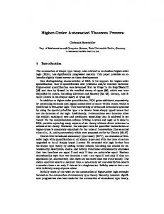
2.1.3 Problem Description by an Example Let us take a look at the screenshots in Figures 2.1. and 2.2. They present part of the contents of two Mathematica notebooks storing text and formulae. The formulae are in predicate logic, in the Theorema external syntax. The formulae and the text in these files are grouped under certain headings in sections, subsections, etc. Such files can either be the result of an automated process, or can be created by a human user, via Mathematica’s and Theorema’s front–end environments. Typing the documents is done in a WYSIWYG style: Both Mathematica and Theorema provide several tools and toolbars for creating documents and typing mathematical formulae in a user–friendly way.

Figure 2.1.

Figure 2.2.

The contents of the first file (Figure 2.1.) describe the basic notions of the tuple theory. It gives the definitions of the tuple concept, the definitions of operations that can be performed on tuples (reversion, concatenation, etc), and propositions involving the defined concepts. The second file

10


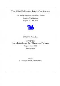
(Figure 2.2.) stores axioms and definitions in the domain of natural numbers, where the natural numbers are expressed by the Peano axioms. Note that this is only a small example. In practice we may have dozens of files, each with hundreds of formulae. Case studies that involve files with a large number of formulae are, for example, the algorithm synthesis [Buchberger&Craciun:03] and the Groebner rings case studies [Buchberger:03b]. We are also working on a large case study in the frame of the CreaComp didactic project that aims at the use of Theorema in math teaching. Let us now assume that we want to investigate some of the properties of the length of tuples. For such a case study we need to use basic knowledge about tuples and natural numbers. Since the two files already contain the formalization of this knowledge, we would like to use this knowledge, combine it, extend it, and produce a third file containing the new knowledge (Figure 2.3.). Furthermore, let us assume that we want to select some of the knowledge contained in some of the files and give it as an input to one of the automated reasoning tools of Theorema.

Figure 2.3.

For doing this, we need means to access the desired knowledge within the given files. The most natural way to access formulae and groups of formulae is access by position in files, by section and subsection headings, keywords or labels. Since this is not yet possible in the current native Mathematica notebooks, we need tools for transforming hierarchical section headings, keywords and individual labels of formulae into unique composite labels, which is one of the main objectives of this chapter.

11


2.2 Description of the Label Management Tools 2.2.1 Starting Point for the Development of the Tools The tools for label management described here, take as input Mathematica notebooks which contain comments in text cells and predicate logic formulae in input cells. The formulae are given in Theorema external syntax. Also, in these notebooks, labels of various kinds (section heading, key words like "definition", "theorem" etc., and individual labels) can be attached to formulae and groups of formulae. For this, we developed a particular Mathematica stylesheet. A Mathematica stylesheet is a special kind of notebook that defines the styles to be used in other notebooks [Wolfram:03, Section 2.10]. By our stylesheet, keywords like "definition", "theorem", "property", etc. can be attached to entire sections, subsections, etc. Formulae that occur under these headings will have attached the keyword given by the style of the headings. If desired, the user can also override these keywords by keywords at the level of individual formulae. With the help of this stylesheet, the label management tools can identify, select, and re–combine formal parts of documents and use them, for example, as input to automated reasoners. The documents processed by the label management tools operate on libraries of Theorema notebooks. A library is a collection of Mathematica notebooks using the above stylesheet. By the tools described below it is guaranteed that the notebook labels are unique. Also, we provide an extra index file that lists all notebooks in the library and also describes the mutual inclusion of notebooks in the library, see below. In addition, the Mathematica package facility is used in the organization of the notebooks in the library for speeding up re–loading of notebooks. In the following, we will describe the main tools which we designed and implemented for achieving the objectives specified in Section 2.1.3 above. For the convenience of the user, these tools can be accessed also by a new Theorema toolbar, called 'Library Utilities'.

2.2.2 Tool for Systematic Generation of Hierarchical Labels An example of a Theorema notebook is given in Figure 2.1. above. It has a notebook title ("Basic Notions: Tuples") and a notebook label ("BN:Tuples"). Formulae, in input cells, are grouped under section and subsection headings. Hierarchically grouping cells in sections, subsections and so on, is a feature of Mathematica notebooks. It is common practice that larger notebooks have chapters, sections and so on, each represented by groups of cells. The extent of these groups is indicated by a bracket on the right. [Wolfram:03] which can also be conveniently used for optical contraction of sections to obtain an easy overview. The headings of the cell groups, the notebook title, the notebook label, and labels of individual formulae are the components used for generating and attaching unique composite labels to all formulae and groups of formulae in the notebook. If the notebook label is not present in the

12


document a notebook label will be generated automatically from the notebook title such that every notebook in the notebook library has a unique identifier. For this reason, the notebook title is a mandatory element in the Theorema notebooks. User given notebook labels are checked against the list of existing notebook labels (extracted from the library index file). The user is notified when the notebook label is already used by another Theorema notebook. From the notebook title, notebook label, section headings, etc. provided by the user our tool automatically generates composite labels for each section, subsection, etc., and individual formula in the notebook. These composite labels are generated in three variants which we call long, short, and decimal composite labels, respectively. The details of this process are described below. In Figure 2.1., for example, the user provided notebook and theory labels. The user also provided all of the headings in the notebook, among them "Operation on Tuples: Concatenation". The generated labels are: "BN:Tuples.Propositions Involving the Definitions Above.Operation on Tuples: Concatenation’’ for the long label variant, "BN:Tuples.ProInvDefAbo.OpeTupCon ’’ for the short label variant, and "BN:Tuples.5.1" for the decimal label variant. The short variant of the label is obtained from the long variant by a simple string truncation algorithm, with some proviso for preserving uniqueness. The period in the above label variants plays the role of a separator, displaying the composite structure of the labels generated. In Mathematica, notebooks are represented as Mathematica expressions. The label generating routine takes as input the Mathematica expression of a Theorema notebook. The notebook expression has a recursive structure, reflecting the grouping and subgrouping of cells in the notebook. Correspondingly the label generating routine proceeds recursively. The label variants are created by concatenation operations, where the operands are, depending on the label variant, the text of the heading, the short text of the headings (obtained by string truncation algorithms), and notebook counters. Eventual user–given labels are taken into account for the generation of the short and long label variants. The notebook label is prepended to each of the labels so that any resulting label we look at, in the Theorema notebook, contains the notebook label as a substring. Because the notebook label is unique among notebook labels in the library, we are sure that the generated labels uniquely identify the formulae and groups of formulae within the library.

13


Figure 2.4.

Figure 2.5.

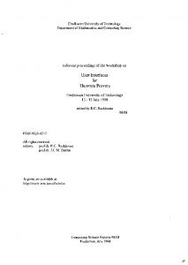
Figures 2.4. and 2.5. show the notebooks in Figures 2.1. and 2.2. after they have been processed by the label generating routine. The labels that can be seen right above the formulae and groups of formulae are the decimal part of the generated labels. The short label variants are not shown. From now on, when we use the word ’label’we refer to one of the three variants of a label. Now, groups of formulae and individual formulae of Theorema notebooks can be referenced by composite labels and can be used for composing new Theorema notebooks and knowledge bases as an input to formal reasoners as described in the next two sections (see Figure 2.3.).

2.2.3 Tool for Including Formal Parts of Notebooks into Other Notebooks When we write a new Theorema notebook we may now also include parts of already existing Theorema notebooks in the library. For this we implemented an ’Include’command which takes all formulae referenced in its arguments and copies them, together with their unique labels, into the current notebook. This gives us the possibility to concentrate knowledge dispersed in various notebooks in the library in one Theorema notebook and use this new notebook independently of the library. Of course, there is also a possibility to list the new notebook in the library index of the current library or some other library. This is particularly convenient when distributing libraries over the web. The ’Include’command has the structure

14


Include#Label1 , Label2 , ..., Labeln , Option',

whose functionality should be self–explanatory: Take the collections of formulae referenced by the composite labels Label1 , ..., Labeln from the current library and copy them into a new version of the notebook that contains the 'Include' command and cancelled the 'Include' command. There are two settings of the 'Option' argument of the 'Include' command. With the first setting, the original composite labels of the formulae included are kept unchanged. With the second setting, the composite label of the 'Include' command will be prepended to the labels of the formulae included. If the no setting for 'Option' is given, the latter setting is considered.

2.2.4 Tool for Using Selected Formal Parts of Notebooks The various reasoners (provers, simplifiers, and solvers) of Theorema can be called by instructions of the following structure Reason#Goal, using KnowledgeBase, by ReasoningMethod',

where 'Reason' can be 'Prove', 'Compute', 'Solve'; 'KnowledgeBase' is expressed by ;

Label1 , ..., Labeln ?,

and Label1 , ..., Labeln are composite labels of collections of formulae in the notebook library. For example, Prove#"LenTpl.3.1", using ;"BN:Tuples", "NN:Basic"?, by TupleEqIndProver',

where 'TupleEqIndProver' is a Theorema prover that combines rewriting and induction over tuples. Alternatively, we also implemented the following 'Theory' construct: Theory#Label,

;

Label1 , ..., Labeln ?',

which is something like a temporary assignment of a new label to specified collections of formulae so that we can formulate calls to reasoners also in the following form: Reason#Goal, using Label, by ReasoningMethod'.

For example, the above call can be formulated in the following way: Theory#"Tuples and Natural Numbers", ;"BN:Tuples", "NN:Basic.1"? ' Prove#"LenTpl.3.1", by TupleEqIndProver, using "Tuples and Natural Numbers"'.

At the implementation level, the selection tool, whose usage is described above, uses a subroutine that translates the formal content of the Theorema notebooks into Theorema internal syntax which is understood by the Theorema provers. This subroutines use Theorema's input parsing routines

15


described briefly in [Windsteiger:01]. The translated knowledge, in Theorema internal syntax, is stored together with the labels attached to it, into Mathematica package files for efficiency reasons. Loading knowledge stored in Mathematica package files is faster than translating the formal knowledge in the Theorema notebooks into Theorema internal syntax. The library index file keeps record of these package files.

2.3 Conclusions to this Chapter We presented simple tools that allow to reference specific parts of collections of mathematical knowledge bases organized in libraries of Theorema notebooks. These tools generate systematically composite hierarchical labels for all the sections, subsections etc. and the individual formulae of Theorema notebooks from section headings and individual labels of formulae in the original notebooks provided by the user. With these tools one then can quickly compose specific new notebooks and knowledge bases as input to the formal reasoners of the Theorema system using the composite hierarchical labels. These tools can also be used for knowledge bases in other systems by translation of the formulae formats between systems. Seemingly, label management is a trivial part of mathematical knowledge management. It also seems that label management in the sense specified in this chapter is not an explicit goal in the current MKM systems (see the overview in Chapter 6 Section 1). However, we believe that, in fact, systematic and efficient label management is quite significant for the user–friendliness of future mathematical knowledge management systems and needs systematic treatment. For different purposes within MKM the choice of labels must meet different criteria. For example, for human readers of mathematical knowledge bases (e.g. in the form of Theorema notebooks), long textual labels may be preferable whereas, in the presentation of proofs, short version of labels are desirable in order not to disrupt the flow of the proof presentation. In the extreme case, if the proof presentation style of 'Focus Windows' is used (see Chapter 5), one even does not need labels in proof presentations. However, at the same time, labels as references for organizing new knowledge bases from given ones, for example as input to provers, are very important. Thus, flexible label management tools on top of the logic tools of MKM systems are necessary.

16


3

3. Interactive Proving in Theorema

3.1 The Problem One of the main goals of the Theorema project is the design and implementation fully automated provers. In this paradigm, the user provides the formula to be proved and the knowledge from which the goal and the prover will either come up with a proof or report that it cannot find a proof. However, interaction of the user with an algorithmic prover at certain situations during the generation of a proof may sometimes be very helpful. Let us try, for example, to prove that the limit of the sum of two sequences of real numbers is the sum of their limits. Formalized in Theorema, this is: Proposition#"limit of sum", any#f, a, g, b', +limit#f, a' Â limit#g, b'/ w limit#f ¨ g, a b' "lim of

¨ '

"

where ’limit’and ’¨’ are defined as follows: Definition%"limit",

f,a

limit#f, a' y

0

N

n n N

#

f n' a H "lim:"

Definition#"sum of sequences", any#f, g, x', +f ¨ g/#x'

)

f #x' g#x' "f

¨

g" '

where ’+’and – are the well known addition and subtraction operations on the reals. Using the Theorema PND prover, which is a general prover for predicate logic, a first proof attempt may be generated by the call: Prove#Proposition#"limit of sum"', using Definition#"limit"', Definition#"sum of sequences"', by PredicateProver';

The (failing) proof attempt is: Prove: (Proposition (limit of sum): lim of ¨)

a,b, f ,g

+

limit# f , a' Â limit# g, b' Á limit# f

¨

g, a b'/ ,

under the assumptions: (Definition (limit): lim:)

-

a, f

limit# f , a' x -H

!

0Á

+

N n

nN

Á

f #n' a H /11 ,

17


(Definition (sum of sequences): f ¨ g)

f ,g,x

++

f

¨

g/#x'

f # x' g# x'/ .

For proving (Proposition (limit of sum): lim of ¨) we take all variables arbitrary but fixed and prove: (1)

limit# f0 , a0 ' Â limit#g0 , b0 ' Á limit# f0 ¨ g0 , a0 b0 ' .

Proving (1) by the deduction rule fails. We assume (2)

limit# f0 , a0 ' Â limit#g0 , b0 '

and show (3)

limit# f0 ¨ g0 , a0 b0 ' .

From (2.2), by (Definition (limit): lim:), we obtain: (5)

-H !

0Á

+

N n

Á

nN

g0 #n' b0 H /1 .

From (2.1), by (Definition (limit): lim:), we obtain: (4)

-H !

0Á

+

N n

Á

nN

f0 #n' a0 H /1 .

Proving (3) by contradiction fails. We assume (6)

»

limit# f0 ¨ g0 , a0 b0 ' ,

and show a contradiction . From (6), by (Definition (limit): lim:), we obtain: (7)

-H ! »

0Á

+

N n

nN

Á +

f0 ¨ g0 /#n' +a0 b0 / H /1 .

Formula (7) is simplified to: (8)

-» -H !

0Á

+

N n

nN

Á +

f0 ¨ g0 /#n' +a0 b0 / H /11 .

By (8) we can take appropriate values such that: (9)

» -H0 !

0Á

+

N n

nN

Á +

f0 ¨ g0 /#n' +a0 b0 / H0 /1 .

Formula (9) is expanded into (10)

H0 !

0Ð

+

N n

nN

Á +

f0 ¨ g0 /#n' +a0 b0 / H0 / .

Formula (10.2) is simplified to: (11)

-» +

n

N

nN

Á +

f0 ¨ g0 /#n' +a0 b0 / H0 /1 .

From (10.1), by (5), we obtain: (13)

+

N n

nN

Á

g0 #n' b0 H0 / .

From (10.1), by (4), we obtain: (12)

+

N n

nN

Á

f0 #n' a0 H0 / .


+

n

n N0

Á

f0 #n' a0 H0 / .


+

n

n N1

Á

g0 #n' b0 H0 / .

The proof of (a contradiction) fails. (The prover "PND" was unable to transform the proof situation.) Ã

18


The reason why the proof attempt fails is manifold. The main reason is that, in fact, the knowledge we provided is not strong enough for proving the goal formula in the exact sense that the goal is not a logical consequence of the knowledge. Hence, as a first interaction of the user, we use a different prover (the "PCS" prover) that, implicitly, uses quite some special knowledge on real numbers and, in addition, applies a particular strategy for handling formulae with operations defined by alternating quantifiers (like " ") as, for example, the operation of ’limit’.The PCS prover (which stands for "Prove Compute Solve") combines predicate logic proving, simplification, and inequality solving over the reals. Its main strategy is the reduction of a proof problem on functions on the reals to inequality solving over the reals. The PCS prover has been proposed B. Buchberger, see [Buchberger:96], and was implemented in the PhD thesis [Vasaru–Dupré:00]. The corresponding prove call in our example is: Prove#Proposition#"limit of sum"', using Definition#"limit"', Definition#"sum of sequences"', by PCS'.

The proof attempt is: Prove: (Proposition (limit of sum): lim of ¨)

f ,a,g,b

+



L M M M M M f ,a M N

¨

g, a b'/ ,

limit# f , a' x


f ,g,x

++

f

f #n' a H /]]] ,

g/#x'

f # x' g# x'/ .

N

n n N

0

¨

\ ] ]

+

] ^

We assume (1)

limit# f0 , a0 ' Â limit#g0 , b0 ' ,

and show (2)

limit# f0 ¨ g0 , a0 b0 ' .

As there are several methods which can be applied, we have several choices to proceed with the proof. Alternative proof 1: failed Formula (1.1), by (Definition (limit): lim:), implies: (3)

N

n n N

0

+

f0 #n' a0 H / .

By (3), we can take an appropriate Skolem function such that (4)

+

n 0 n N0

f0 #n' a0 H / ,

As there are several methods which can be applied, we have several choices to proceed with the proof. Alternative proof 1: failed Formula (1.2), by (Definition (limit): lim:), implies: (5)

0

N

n n N

+

g0 #n' b0 H / .

19



+

n 0 n N1

g0 #n' b0 H / ,

As there are several methods which can be applied, we have several choices to proceed with the proof. Alternative proof 1: failed Formula (2), using (Definition (limit): lim:), is implied by: (7)

N

n n N

0

++

f0 ¨ g0 /#n' +a0 b0 / H / .

We assume (8)

0,

H0 !

and show (9)

N

n n N

++

f0 ¨ g0 /#n' +a0 b0 / H0 / .

As there are several methods which can be applied, we have several choices to proceed with the proof. Alternative proof 1: failed The proof of (9) fails. (The prover "QR" was unable to transform the proof situation.) Alternative proof 2: failed We have to find N2 such that (10)

+

n

n N2

Á +

f0 ¨ g0 /#n' +a0 b0 / H0 / .

Formula (10), using (Definition (sum of sequences): f ¨ g), is implied by: (11)

+

n

n N2

Á +

f0 #n' g0 #n'/ +a0 b0 / H0 / .

The proof of (11) fails. (The prover "QR" was unable to transform the proof situation.) Alternative proof 2: failed The proof of (2) fails. (The prover "NDS" was unable to transform the proof situation.) Alternative proof 2: failed The proof of (2) fails. (The prover "NDS" was unable to transform the proof situation.) Alternative proof 2: failed The proof of (2) fails. (The prover "NDS" was unable to transform the proof situation.) Ã

The PCS prover also failed to prove this conjecture. The next type of user interaction is adding the appropriate knowledge to the knowledge bases. In our example, by examining the last proof attempt, especially formulae (11), (4) and (6), we conclude that additional knowledge about modules and distances between points (expressed by modules) may help: Lemma$"distance of sum", ++x z/ +y t/ +G H// u +x y G Â z t H/ "dist " (

x,y,z,t, ,

Prove#Proposition#"limit of sum"', using Definition#"limit"', Definition#"sum of sequences"', Lemma #"distance of sum"', by PCS'

20


The proof attempt is (for a better overview, we have omitted the proof steps that were already presented in the previous proof attempt): Prove: (Proposition (limit of sum): lim of ¨)

f ,a,g,b

+


under the assumptions:

L M M M M M f ,a M

(Definition (limit): lim:)

N

¨

g, a b'/ , \ ] ]

+

f #n' a H /]]] ,

¨

g/#x'

f # x' g# x'/ ,

x z/ + y t/ G

H/

limit# f , a' x

N

n n N

0


f ,g,x

++

f

]

^

(Lemma (distance of sum): dist+)

x,y,z,t, ,

+

x y G

Â

z t H

Á +

.

We assume (1)


and show (2)

limit# f0 ¨ g0 , a0 b0 ' .

(... omitted proof steps ...) We have to find N2 such that (10)

+

n

n N2

Á +

f0 ¨ g0 /#n' +a0 b0 / H0 / .


+

n

n N2

Á +

f0 #n' g0 #n'/ +a0 b0 / H0 / .

Formula (11), using (Lemma (distance of sum): dist+), is implied by: (12)

+n N2 , n

Á

f0 #n' a0 G

Â

g0 #n' b0 H / .

0

As there are several methods which can be applied, we have several choices to proceed with the proof. Alternative proof 1: failed The proof of (12) fails. (The prover "QR" was unable to transform the proof situation.) Alternative proof 2: failed We have to find (13)

G0

, H1 , and N2 such that

+G0 H1

H0 / Ð +

n

n N2 Á f0 #n' a0 G0 Â g0 #n' b0 H1 / .

Formula (13), using (6), is implied by: +G0 H1

H0 / Ð +

n

n N2

Á H1 !

0 Â n N1 #H1 ' Â f0 #n' a0 G0 / ,

which, using (4), is implied by: (14)

+G0 H1

H0 / Ð +

n

n N2 Á G0

!

0 Â H1

!

0 Â n N0 #G0 ' Â n N1 #H1 '/ .

As there are several methods which can be applied, we have several choices to proceed with the proof. Alternative proof 1: failed The proof of (14) fails. (The prover "QR" was unable to transform the proof situation.)

21


Alternative proof 2: failed Formula (14) is implied by (15)

+G0 H1

H0 / Ð G0 !

0 Ð H1 ! 0 Ð +n N2 n

Á

n N0 #G0 ' Â n N1 #H1 '/ .

The proof of (15) fails. (The prover "QR" was unable to transform the proof situation.) Ã

We can, again, examine the proof attempt to decide on how to continue in order to obtain a proof of the given proposition. We can either add more lemmata to the knowledge base used by the prover, or use a different prover and/or different proof strategies of the chosen prover. Following the first alternative, we can formulate the required knowledge (as lemmata, propositions, definitions, etc.) and call the prover again, where the knowledge base used by the prover is now enlarged to contain the new knowledge. The last proof attempt in the above example illustrates this procedure. We can repeatedly call the prover, each time with some new knowledge added to the base used by the prover, until hopefully a proof or disproof of the conjecture is obtained. However, this style of work (attempt to find a proof, add more knowledge, restart the proving process) is, of course, not really economic. Rather, we want to introduce new knowledge right at the time when the proof fails and continue the proof from this point on. In the case we want to use a different prover of the Theorema system we have to modify the ’Prove’call so that it invokes a different prover of the Theorema system. In the example above, we have first used the ’PredicateProver’and then the ’PCS’prover. Now, each prover of the Theorema system comes with a set of options that give users the possibility to indicate certain strategies to be applied during a proof search. The options have default values. For all that, their values do not change during a proof search, so users of the system cannot, for example, chose to first apply one strategy, and then continue with another. From the outset, Theorema’s current provers are designed to work in an automatic style: they take as input a goal formula to be proven and a (possible empty) list of assumption formulae to be used for proving it. The prover can be ’tuned’ via its options, but no other operation can be performed by the user once the ’Prove’call is sent to the Mathematica kernel for evaluation. The result of this automated proof search process is presented then to the user in a natural language style. If the proof is unsuccessful the user, as in the alternatives presented before, re–starts the proof search process, on different premises (additional knowledge, different options of the used prover, different prover of Theorema). However, we would like to have the possibility to guide the proof search routines during the proof search. For example, we would like to hint the prover to use certain instances for specific quantified variables at various points in the proof. In the proof attempt above, for instance, we would like to hint the prover to use cccc20cc for each G0 and H1 in formula (13), where H0 is introduced by formula (8). In other words, we are interested to have an interaction between the user and the Theorema system amid the development of proofs. In the following sections we will describe the tools that support such a user–system interaction.

First attempts to integrate interactivity into Theorema were done by Tudor Jebelean (a core member of the Theorema group) and are described in [Buchberger&al:98]. Some of the ideas in

22


this work were taken as the starting point of the work in this thesis. Prior to this work, in [Tomuta:98] is shown how interactive proving was to be integrated in the architecture of Theorema, but very little implementation was done. Another attempt to provide user–system interaction is described in [Nakagawa&Kossak:99]. Felix Kossak, in [Kossak:99], further develops the prototype presented in [Nakagawa&Kossak:99]. The set of tools we have implemented form an environment that we will refer to as the "interactive environment", from now on. Proving within this environment will be called proving in the "interactive mode", while the default proving mode in the Theorema system will be called proving in the "non–interactive mode".

3.2 Description of the Tools 3.2.1 Preliminaries The interactive environment allows a finer grained interaction between a human user and the Theorema system. When the environment was designed we had in mind three groups of users. For the first group of users, the environment has a didactical value: it can be used to train formal proving, only allows correct operations and never gets tired. The second group of users are those who are already familiar with formal proving techniques and with the details of the Theorema system. For them, the interactive environment enriches the proving power of the Theorema system, by allowing them to use their creative ideas and intuition (for example, instantiating quantified variables with certain values). The third group of users is the Theorema developers group, for which the environment can be used as a tool for testing the provers that are still in development.

23


In the non–interactive mode, the Theorema provers apply the inference rules automatically. The inferences are repeatedly applied until either a proof is obtained or no inferences can be applied anymore. The users only see the final output of this process. In contrast, when searching for proofs in the interactive environment, the system is compelled to stop after each application of an inference rule, to present the produced proof sofar, and to wait for a decision from the side of user. In the interactive mode, the proofs are gradually developed starting from an initial proof tree that has two nodes: the root node that contains the proof problem as given by the user (goal formula and assumption formulae, if any), and a child node, which contains the proof problem as in the root node and, additionally, internal information, specific to the provers and to the proof search routines of Theorema. The child node is an unexplored node, or in Theorema terminology: a pending node. The information stored in an unexplored node is called a "proof situation". The node expansion is done by calling a prover to apply one of its inferences on the proof situation of the node to expand. An inference rule application will produce none, one or more proof situations that are inserted into the proof tree as unexplored children of the expanded node. The proof search mechanism will add to the information stored in the expanded node a trace of the inference rule application. While the system waits for a user decision to continue, in the interactive mode, the user can perform one or more of the following actions: • select a proof situation in the proof; • inspect a selected proof situation; • add or remove assumptions in a selected proof situation; • suggest instances for universally or existentially bound variables; • add or remove branches in the proof tree; • choose one among different provers to continue the proof, eventually change its options; • make the system expand the proof by one inference rule application; • ask the system to finish the proof without anymore user interventions; • put an end to the proving session and exit the environment. The components of the interactive environment which realize the concrete execution of the above user actions can be grouped in three categories: • working notebook files; • developer information and log windows; • menu–palette windows (also called toolbars).

24


3.2.1.1 Working Notebook Files In this category fall the Mathematica notebook files in which the user writes and stores the mathematical knowledge used during a proving session (interactive or not). A special notebook is "The Proof Window" which is used for presenting the proofs generated by the Theorema provers. In the non–interactive mode this notebook displays the proof in a natural language style. The proof cannot be modified anymore. In the interactive mode, "The Proof Window" displays the sofar developed proof, which can be modified via the tools of the interactive environment. By combining selection of cells in the working notebooks and button clicks on the menu–palettes of the interactive environment, the user can navigate inside the proof–tree, in order to continue the proof on a certain branch, introduce new branches, add/remove assumptions, instantiate variables, etc. 3.2.1.2 Developer Information and Log Windows These windows are used to display environment specific and proof specific information. Their content does not directly influence the proving process. The interactive environment makes use of one log window and one developer information window. The log window records the main commands of the user, displays messages about the interactive environment status and eventual warnings. The developer information window is used to display (on user request) the information stored in the nodes of the proof–tree. This information can be displayed both in a user–friendly external and in Theorema internal form. In addition to these two windows, the environment uses notification dialogs to inform the user that an action she performed is not accepted by the system. 3.2.1.3 Menu–palette Windows The menu–palette windows (also called toolbars) are an important component of the interactive environment. The commands triggered by the buttons on these toolbars allow the user to guide the proof development. Some of the commands require arguments which are provided by prior selections in the working notebooks (e.g. 'New Goal' needs a formula as an argument, 'Start' needs a 'Prove' command as an argument, etc.). There are five toolbars which help the user to carry out the actions listed at the beginning of this section. We give now a brief description of these toolbars and of the functionality of their buttons, more details being given in the next section of this chapter in Section 3.2.2. • The "Theorema Interactive" toolbar (Figure 3.1.a.) contains the main commands for controlling the development of the proof in the interactive mode. These commands are 'Start', 'Next', 'Finish' and 'Stop'. The 'Start' command will trigger the execution of a 'Prove' call, in the interactive mode. The 'Next' command will ask the proving system to expand the selected proof situation

25


by one inference rule application. (The inference rule is automatically chosen by the current prover.) The ’Finish’command will signal the proof search routines to automatically expand the pending nodes in the current proof until either a successful or failed proof is obtained. The ’Stop’ command will abort the current proof development and reset the environment, preparing it for a new prove session. Additionally, the "Theorema Interactive" toolbar has buttons that toggle the display of the "Advanced Proof Operations", of the "Prover", and of the "Debug" toolbars, a button that toggles the interaction mode on and off, and an ’Exit’button for closing the interactive environment. • The "Advanced Proof Operations" toolbar (Figure 3.1.b.) is shown by pressing the 'Advanced Op' button on the "Theorema Interactive" toolbar. Pressing this button again will hide the "Advanced Proof Operations" toolbar. All of the operations triggered by the buttons on this toolbar need, among their input parameters, a pointer to a proof situation in the proof–tree of the current proof. This pointer determines where the next operation will be performed. The pointer can be set using the 'Set Focus' button, which takes as input a cell selected in "The Proof Window". The ' Inst' button helps the user instantiate existentially quantified variables, while ' Inst' does the same for universally quantified variables. '+ Branch' creates and alternative branch in the proof–tree, while '– Branch' removes a branch in the proof–tree. '+ Assm' triggers the insertion of a formula into the list of assumptions of the selected proof situation (i.e. where the focus is set). '– Assm' button triggers the removal of an assumption formula from the list of assumptions of a focused proof situation. For a formula in a selected cell in some working notebook, the function called by the 'New Goal' button will add a new branch in the proof object, where the respective formula is set as the current goal, while on the already existing branches the formula is added as an assumption.

a.

b.

Figure 3.1: a. The "Theorema Interactive" toolbar; b. The "Advanced Proof Operations" toolbar.

• The "Theorema Provers" toolbar (Figure 3.2.a.) allows the user to select a domain–specific prover to be used for the next proving steps. The currently selected prover is marked with red on this toolbar. The "Prover Options ... " button opens a prover specific palette ("Prover Options ...") which allows the user to alter the options of the currently selected prover.

26


a.

b.

Figure 3.2: a. The "Theorema Provers"; b. The "Prover Options ... " toolbars.

In Figure 3.2. we see that the currently selected prover is the prover for Predicate Logic and on the "Prover Options ..." menu–palette we see that the 'TryAlternatives' option is in bold fonts which mean that its value is 'True'. (This option, when set to 'True' will instruct the 'PredicateProver' to try to prove each of the disjuncts in a disjunctive goal.) • The "Debug" toolbar (Figure 3.3.) gives users the possibility to display, for a selected proof situation in the proof–tree, the content of the proof situation. Namely, it can display the current goal formula, the assumption formulae for the selected proof situation. The information displayed when pressing the '•lf Goal', '•asml', '•prinfo', '•af' and 'Focused Position' buttons is especially of interest for the developers of the Theorema system and is described in the subsections below.

Figure 3.3: The "Debug" toolbar.

In the next section we describe in detail how each of the actions triggered by the buttons on the described toolbars are carried out.

3.2.2 Using the Environment For illustrating the operations performable in the interactive proving mode we will use a simple theorem on quantifiers: Theorem%"Simple Example", -- P#x'1 Á Q1 w - +P#x' Á Q/1). x

x

We chose an easy example because we want to focus on the description of the interactive environment rather than on the proof of the theorem itself. We will use this example throughout the remainder of this section. After initializing the Theorema environment, the user can, at any time, open the toolbars that enables him to use the interactive environment by the following call:

27


+

Initialize the Theorema environment / Theorema‘; + open the interactive environment / StartInteractive# ';

The desktop of the user will look, now, similar to the one in Figure 3.4:

Figure 3.4: The initial screen in the Interactive environment.

In Figure 3.4 we can see the "Theorema Interactive" toolbar, a working notebook, ’Interactive Example.nb’, and the Log Window which is empty for the moment. All other toolbars can be brought onto the desktop by pressing their corresponding button (’Advanced Op’ for the "Advanced Proof Operations" toolbar, ’Provers’ to obtain the "Theorema Provers" toolbar, and ’Debug’to display the "Debug" toolbar.) Leaving the interactive environment is done by pressing the ’Exit’ button, which will cause all the objects belonging to the interactive environment to be hidden except for the notebooks that were previously open (like the ’Interactive Example.nb’). The ’On/Off’button is used to temporarily turn off the interactive proving mode, without hiding all the environment’s components. Notice that some of the buttons on the "Theorema Interactive" toolbar are grayed out and cannot be pressed. They will become active when a proof is started. From now on we assume that the toolbar "Theorema Interactive" is always visible on the user’s desktop when working within the interactive environment.

28


3.2.2.1 Setting the Action Focus In the interactive mode, after each completed proof step, the user must decide which action to carry out next (add an assumption, instantiate variables, let the chosen prover perform one inference step, change the active Theorema prover, etc. See the following subsections). Several of these actions require that the user first specifies where in the proof the actions should be carried out, i.e. where the "Action Focus" is. In other words, the user has to have the possibility to select nodes in the proof–tree. The 'Set Focus' button on the "Advanced Proof Operations" toolbar is providing this possibility. We say that a node that is selected has the "Action Focus" set on it. At any given time in the interactive proving mode, "The Proof Window" shows a natural language representation of the current proof–tree. It is natural to expect, then, that selecting cells in this window will also set the Action Focus on the underlying nodes in the proof–tree. This behavior can be realized with the help of the 'Set Focus' button: The user selects a cell in "The Proof Window", by a click on the cell bracket, and presses then the 'Set Focus' button. (In Mathematica, selecting cells in notebooks is done by a click on the cell's bracket). This will trigger the execution of a routine that searches, in the current proof–tree, the node that contains the information displayed in the selected cell. When the node is found the Action Focus is set to it. There are two restrictions that the user has to consent with. First, the only cells that can be selected are cells that contain formulae and cells that represent pending nodes (they have a gray background). Second, multiple cell selection is not allowed. 3.2.2.2 Main Operations: Start, Next, Finish, Stop To start a proof session in the interactive mode the procedure is as follows: the user selects a cell that contains a 'Prove' call. Now, a click on the 'Start' button of the "Theorema Interactive" toolbar will start the proof attempt. The user will see "The Proof Window" display the initial proof situation. The 'Prove' command that was called in our example can be seen in Figure 3.4. The initial proof situation contains the goal to prove and no other assumptions. Notice now that the 'Next', 'Finish' and 'Stop' buttons are active.

29


Figure 3.5: Starting a proof attempt.

The proof tree created by carrying out this operation contains two nodes: the root node, stating the initial proof situation, and its child node, which is a pending node (i.e. not yet expanded). In "The Proof Window" this node is represented by a cell with a gray background (see Figure 3.5.). If we click on the ’Next’ button, the ’PredicateProver’ (which was chosen to prove this theorem) will expand the pending node by an application of one inference rule. In our example, the prover applied the deduction rule. Namely, it assumed that the left hand side of the implication in the goal formula is true, the new goal to prove is now the right hand side of the implication. The result of this inference application is displayed in "The Proof Window" (see Figure 3.6.). By default, a proof that has more than one pending node in the proof–tree is expanded by expanding the left–most pending node in the tree. In "The Proof Window" this node corresponds to the first cell with a gray background, when the window is parsed top–down. If the user whishes to continue the proof on a different branch she has to set the Action Focus to the pending node of that branch, prior to the click on the 'Next' button. Further clicks on the 'Next" button will expand the proof on the branch of the selected node, until either the branch cannot be expanded anymore, or the user decides to continue the proof exploring on a different branch. (In "The Proof Window" branches are illustrated by group cells, the extent of a group is indicated by a bracket on the right. See Figure 3.11. below.)

30


Figure 3.6: The Next step in the proof.

The ’Finish’ button indicates the proof search routines to continue the expansion of the proof without any intervention from the user. The result of this action, in our example is the following successful proof (which is the content of "The Proof Window", after the proof search routines are done): Prove: (Theorem (Simple Example))

-

x

P#x' Á Q1 Á +P# x' Á Q/ , x

with no assumptions. We prove (Theorem (Simple Example)) by the deduction rule. We assume (1)

x

P# x' Á Q

and show (2)

+

x

P#x' Á Q/ .

Formula (2) is transformed into: (3)

+»

x

P# x' Á Q/ .

Formula (3) is transformed into: (4)

+»

x

P# x'/ Î Q.

We prove (4) by proving the first alternative negating the other(s). We assume (6)

»

Q.

We now show

31


(5)

+»

x

P# x'/ .

From (6) and (1) we obtain by modus tollens (7)

»

x

P# x ' .

Formula (7) is simplified to: (8)

+»

x

P# x'/ .

Formula (5) is true because it is identical to (8). Ã

The ’Stop’ button on the "Theorema Interactive" toolbar will clear "The Proof Window" of its actual content, and will prepare the interactive environment for a new proof session. 3.2.2.3 Displaying Information (not only) for Developers The natural language representation of the proof–tree does not show all the content of the proof nodes. The reason for this is that part of the information stored in the nodes is not relevant for the user, but only for the provers of the system. The information displayed to the user is describing the way an inference rule was applied on a certain proof situation. (An inference application involves, normally, only a few formulae from the set of available formulae at a position in the proof–tree.) Other information stored in the nodes of the proofs is prover specific, like the fact that certain formulae are already matched against others for the application of a certain inference rule. However, in the interactive proving mode it is often the case that we are interested in the whole content of the proof node. We may want to know, for example, which are the formulae that are or were available when an inference rule was applied. The developers of the Theorema system may want to check the prover specific information to help them to develop and improve their provers. For this reasons, we have implemented a set of routines that access and display the additional information stored in a node. These routines are triggered by clicks on the buttons of the "Debug" toolbar. Each routine extracts and presents the content of a node that has the Action Focus set on it. These routines display the extracted information in a special window, called "Debug Messages". From left to right on the "Debug" toolbar, these routines do the following: • display the goal for the selected proof node: The 'Goal' and '•lf Goal' buttons trigger routines that extract the goal formula of the proof situation stored in the user selected proof node. The display of the formula is done in a user–friendly form when the 'Goal' button is pressed, and in Theorema internal form when the '•lf Goal' button is pressed. For example, when the Action Focus is set on the pending node of the unfinished proof shown in Figure 3.6. (the cell with the gray background), the user–friendly external and the Theorema internal form of the goal of the node are displayed in the "Debug Messages" window like this:

Goal at the selected proof step :

32


(2)

+

x

P#x' Á Q/

Goal at the selected proof step : •lf %"2", +P#x' Á Q/, •finfo#') x

• display the list of available assumptions: The 'Assm List' and '•asml' buttons trigger routines that extract the list of assumptions stored by the user–selected proof node. The assumptions are displayed in a user–friendly form when the 'Assm List' button is pressed, and in Theorema internal form when the '•asml' button is pressed. For the Action Focus set as in the example above, the assumptions displayed in the "Debug Messages" window are:

Assumptions in the proof situation at selected proof step : (1)

x

P# x' Á Q

in the user–friendly style, and

Assumptions in the proof situation at selected proof step : •asml%•lf %"1", P# x' Á Q, •finfo#')) x

in the Theorema internal style. Note that, in this example and at this point in the proof, the only assumption available is the temporary assumption that was made by the application of the deduction rule in the previous proof step. • display the proof information: When an inference rule is applied, trace about how it was applied, which formulae it used and generated is stored in the nodes of the proof–tree. This trace is called 'proof information' and is used for generating the natural language presentation style of the proof, which is shown in "The Proof Window". The nodes of the proof–tree that were not yet expanded do not have a trace information. The 'Proof Info' and '•prinfo' buttons trigger routines that extract the proof information (if available), and display it to the user. The proof information is presented in a user–friendly form when 'Proof Info' is pressed, and in Theorema internal form when '•prinfo' is pressed. If the proof information is not available (when the selected proof node is a pending node) the routines display a message stating this fact. In the example above, the Action Focus is set on the pending node of the unfinished proof. In this case there is no proof information to display, because the node was not yet expanded. (No inference rule was yet applied that would have left a trace of its application.) Let us set the Action Focus on the node that contains information about formula

33


(2). For this, we select the cell that contains formula (2) (in "The Proof Window") and click on the ’Set Focus’ button. If we click now on the ’Proof Info’ button the "Debug Messages" window will show the following:

The Proof Information at the selected proof step : Inference Rule Keyword : ProveImplication Used Formulae Labels : Theorem +Simple Example/ Generated Formulae : P#x' Á Q,

(1)

(2)

+

x x

P#x' Á Q/.

and by clicking on the '•prinfo' button, the following will be displayed in the "Debug Messages" window:

The Proof Information at the selected proof step :

"ProveImplication", •usedFormulae#"Theorem +Simple Example/"', •generatedFormulae%•lf %"1", P#x' Á Q, •finfo#'), •lf %"2", +P#x' Á Q/, •finfo#'))! x

x

The three parts of the proof information above, namely the inference keyword, the labels of the formulae used, and the formulae generated, are present for all the traces created by any given inference rule throughout the provers of the Theorema system. Some inferences may leave additional traces in the proof information. Take, for example, the ’PCS’ inference rule that is applied when an assumption formula is an instance of an existential goal formula. When this inference rule is applied to a proof situation, the proof search mechanism stores in the proof information, additional to the three parts above, facts about the substitution that unifies the two formulae. All these will also be displayed in the "Debug Messages" window when one of the ’Proof Info’ or '•prinfo' buttons are clicked on. • display the proof situation: The 'Proof Situation' button triggers a routine that extracts the proof situation at the selected node in the proof–tree. This includes the goal formula, the list of assumption formulae, and prover specific facts. The '•af' button triggers the display of the prover specific facts, only. For both of these buttons, the displayed data is in Theorema internal form. Below is shown the proof situation for the already selected node in the example considered in this section:

Proof Situation at the selected proof step :

34


•lf %"Theorem +Simple Example/",

-

x

P# x' Á Q1 Á +P#x' Á Q/, •finfo#'), x

•asml#', •lkTab%"ProversHistory", , "LastProver", PND,

"PND", •lkTab%"ModusPonensFacts", •lkTab#',

"MatchingFacts", •lkTab#', "NewFormulae", , •oldForms#',

"GoalHistory", - P# x' Á Q1 Á +P#x' Á Q/!!!)!!) x

x

!

Please observe the difference between the proof situation and the proof information of a node in the proof–tree. The proof situation contains a goal formula and a possible empty list of assumptions, together with prover specific facts, while the proof information contains the trace of applying an inference rule to this proof situation. • display all assumptions: The inference rules of the Theorema provers transform the proof situation they are applied to into other proof situations. It is often the case that inferences which rewrite formulae among the assumptions of a proof situation replace the formulae with the newly inferred ones. Therefore, formulae which occurred in the list of assumption formulae of a node in the proof–tree may not occur anymore in the list of assumption formulae of a descendant node. The 'All Assumption' button calls a routine that extracts all the formulae that occurred as assumptions during the proof prior to the selected node in the proof–tree. The formulae are displayed in the "Debug Messages" window in the user–friendly style. • display the position of the node where the Action Focus is set: 'Focused Position' displays the position of the selected node in the proof–tree. The position is relative to the style Mathematica organizes and stores expressions. The developers of the Theorema system can use the displayed position for directly manipulating the data structure that holds the proof–tree, using special Theorema and Mathematica function calls which we do not describe here. In our example, the position of the node which has the Action Focus set is: The Current Focused s Selected Position :

2, 1, 2, 1, 2, 1, 2, 1, 2, 1, 2, 1, 2, 1

35


3.2.2.4 Adding and Removing Assumptions In the introductory example of this chapter we have seen that, in the non–interactive proving mode, all the knowledge that might be needed to obtain a successful proof of a conjecture has to be provided beforehand, at the time the proof search process is started. In contrast, in the interactive mode the user of the Theorema system can start with some assumptions and, as soon as she sees the need for it, may add assumption formulae to the proof situation of an unexpanded node. This can be done in the following way: • First, the user has to make sure that the Action Focus is set on an unexpanded node in the proof–tree. If the Action Focus is not correspondingly set and the user still tries to add the assumption, a notification window with a message will appear, asking the user to set the focus correctly. • Second, the user has to select the cell with the formula she wants to add to the proof situation of the selected pending node. The formula has to be given in the Theorema language, as a Lemma, Proposition, Definition, etc. After selecting the cell, the user has to click on the '+ Assm' button on the "Advanced Proof Operations" toolbar. When the '+ Assm' button is clicked the selected pending node will be expanded. The proof information of the expanded node is generated by the routine attached to the button and has the same structure with the proof information produced by an inference rule of a Theorema prover. The new pending node is a child of the expanded node and will contain a proof situation derived from the one of the expanded node by adding to its assumption formulae the formula added by the user. This can be easily checked by using the buttons on the "Debug" toolbar (Section 3.2.2.3) to display the new proof situation. The screenshot in the Figure 3.7. shows the working notebook "Interactive Example.nb" that contains a lemma "Instance", in Theorema language, whose formula is labeled "I1". The user has added this lemma to the proof situation of the pending node shown in Figure 3.6. The result is shown in "The Proof Window" in Figure 3.7. (the notebook partially behind the "Interactive Example.nb" notebook). Dual to the assumption addition operation, we provide the user with a formula deleting operation, which allows her to remove assumptions from a proof situation. Discarding assumptions can be done when the user considers that certain formulae will not contribute to the proof development.

36


Figure 3.7: Added assumption "I1".

Assumptions can be removed only from a proof situation of an unexpanded node in the proof–tree. Removing assumptions is done following the same procedure as adding them: the user has to set the Action Focus on a pending node, select the formula she wants removed, and then click the '– Assm' button on the "Advanced Proof Operations" toolbar. The formula to be removed must be selected in the "Debug Messages" window, where the user has previously displayed the list of assumptions for the selected pending node, in the user–friendly style (see 'Assm List' description in Ssection 3.2.2.3). The routine that deletes the indicated assumption formula from the proof situation of the selected pending node will first check that the formula, indeed, occurs among the assumptions of the proof situation.

Figure 3.8: Removed the assumption "I1".

37


In Figure 3.8. we can see the outcome of removing the formula "I1" from the proof situation of the unexpanded node in figure 3.7. Selecting the formula to be removed was done in the "Debug Messages" window (also shown in Figure 3.8.). 3.2.2.5 Instantiate Quantified Variables One of the specific difficulties in algorithmic proof generation is finding appropriate instances for quantified formulae. Within the interactive environment we give the user the possibility to propose instances in these situations. To instantiate a universally or existentially quantified variable the user has to select in "The Proof Window" the quantified formula and click on the ’ Inst’ or ’ Inst’, respectively. A window will appear where the user can type in a substitution for the variables she whishes to instantiate. The substitution has the syntax ’{variable_list} | {term_list}’. The number of variables has to coincide with the number of terms. It is not necessary that the variables given in this window occur in the formula for which the user gives a variable substitution. The variables that do not occur in the formula will be ignored by the instantiation routines. In Figure 3.9. the user instantiates variables x and y in formula (2). The instantiation routine will, of course, ignore the variable y which does not occur in formula (2). The result of the instantiation is shown in Figure 3.10. Note that, even though the variable y is ignored when the instantiation in formula (2) is performed, the given substitution shows all the user given variables.

Figure 3.9: Instantiating the variable in the goal.

38


Figure 3.10: The result of variable instantiation.

Of course, the user can instantiate existentially quantified variables only if they occur in a goal formula and universally quantified variables only if they occur in assumption formulae. 3.2.2.6 Add/Remove Branches, Insert a Goal Formula For the case the user wishes to work on an alternative proof of a goal of a proof in development, within the same interactive proving session, the interactive environment provides her with the possibility to add branches at any position in the proof–tree, except for the root. The button '+ Branch' on the "Advanced Proof Operations" toolbar implements this facility. To add a branch at some point in the proof, the user has to select a formula cell in "The Proof Window" and click on the '+ Branch' button of the "Advanced Proof Operations" toolbar. The routine triggered by this button will insert two nodes in the proof–tree. One node is inserted as a child of the node that was selected in "The Proof Window". (Recall that such a selected node has the Action Focus set.) The node will have, then, two sub–trees: The first one is the sub–tree of the node with the Action Focus set, the second sub–tree is a pending node, which is the second node inserted by the routine in the proof–tree. The proof situation of the inserted pending node duplicates the proof situation of the node with the Action Focus set. In this way, the user can continue to develop the proof with the sofar derived formulae available on the added branch as well.

39


Figure 3.11: A new branch was added to the proof–tree.

Using the simple example of this section, Figure 3.11. shows that the user (after a few proof steps were executed) decided to investigate how the proof develops if the lemma "Instance" is added to the proof situation. In order not to overwrite the existing proof steps, a new branch is added immediately after the generation of formula (2). Then, the user set the focus on the pending node of the new branch, and added the lemma "Instance", whose formula is labeled "I1". The user can continue to develop the proof on any of the two branches, provided that the Action Focus is set correspondingly to the pending node of one branch or the other. Within the interactive environment, the user also has the possibility to delete entire branches from a current proof–tree. For example, if the user decides that a proof alternative she was working on does not lead to a successful proof, she can delete it so that the proof contains less unuseful information. To delete a branch in the proof–tree, the user has to select a formula cell that belongs to the undesired branch. When the '– Branch' button on the "Advanced Proof Operation" toolbar is clicked, the branch will be deleted. The 'New Goal' button on the "Advanced Proof Operation" toolbar combines the branch addition and assumption addition operations in the following way: If the user selects a cell containing a formula (in Theorema language) in any of the working notebook files and then clicks the 'New Goal' button the triggered routine adds a new branch to the proof–tree after the node

40


with the Action Focus set. The second branch will contain the formula as an assumption, while the first branch will contain the formula as a goal to be proven. In other words, the added formula can be used in proving the original goal if it can be, in turn, proved.

Figure 3.12: Adding a new goal to the proof.

Figure 3.12. shows the outcome of using the ’NewGoal’routine. The goal for the first branch is formula (I1) while, on the second branch, the goal is formula (4) and formula (I1) is among the assumptions of the pending node.

41


3.2.2.7 Change Provers, Set Prover Options The Theorema system has different provers for different mathematical domains and theories. In the non–interactive proving mode, the prover called to find a proof for a conjecture remains fixed during the whole proof search process. In the interactive mode, the user can call the application of the various domain specific provers within the same proof search process. The selection of the different provers is done by a click on one of the buttons on the "Theorema provers" toolbar, at any time during an interactive proving session. We have said before that each of the Theorema provers comes with a set of options which can guide the prover in finding a proof of a conjecture. In the non–interactive proving mode these options are fixed for the duration of the proof search. In contrast, in the interactive mode we can change the values of these options during a proof session. The "Prover Options ..." button on the "Theorema provers" toolbar will dynamically create another toolbar, "Prover Options" which contains a button for each of the options of the currently selected Theorema prover. Setting prover options whose possible values are 'True' or 'False' can be done by a click on the name of the option. The option name will appear in bold face when set to 'True', and plain face when set to 'False'. For the options that take other values than 'True' or 'False', a click on their name will open a small dialog window where the user can type in the value of the option.

3.2.3 Comments on Implementation One crucial matter of interactive proving is to make the proof search routine stop after a certain number of inference rule applications and await input from the user. The solution chosen in earlier implementations was to suspend the execution of the proof search routine, after one inference rule application, to allow user input. This was done by starting a Mathematica subprocess that collected the user actions. Unfortunately, closing the subprocess to continue the proof search was not a clean operation due to a bug in Mathematica (version 3.0 for Linux and Unix) [Kossak:99]. Several workarounds had to be implemented to ensure that the user input was not lost. In the current implementation we have opted for a different solution. We have introduced a system–global boolean variable which keeps track on the current proving mode (interactive or non–interactive), and a step–counter that controls the number of proof steps to be performed by the proof search routine. In the non–interactive proving mode, the step–counter variable is ignored and the proof search routine proceeds until either a successful proof is obtained or no inference rule can be applied anymore. In the interactive mode, every time the proof search routine is invoked the step–counter is, first, set to a predefined value. With each inference rule application this value is decreased by one. As soon as the step–counter reaches zero, the proof search routine stops, and returns the proof developed sofar which is, then, presented to the user, in "The Proof Window". The user can modify the proof via the tools of the interactive environment. When the 'Next' button on the

42


"Theorema Interactive" toolbar is clicked the proof search routine is invoked to further expand the proof. The expansion is done for the left–most pending node in the proof–tree, unless otherwise indicated by the user (see Section 3.2.2.2). The value of the step–counter in the current implementa tion is set to 1, which means that the proof search stops after one inference rule application. We mention here two important advantages of this solution. One is that only few modifications of the main proof search routines of the system were necessary: First, a check of the step–counter value was added to the termination conditions of the proof search routine and, second, certain Theorema specific variable initialization are by–passed when the proof search is invoked in the interactive mode. (For example, we do not want the proof–tree to be initialized to an empty one, as in the non–interactive mode, but we want to expand it further). The second important advantage of the solution chosen by us is that no alteration of the existing provers of the Theorema system had to be done in order to use them for proving in the interactive mode. From the outset, Mathematica is not an environment for developing user interfaces. Therefore, the elements of the interactive environment interface do not include objects like drop–down lists, dynamic menus, context–sensitive menus, check boxes, etc. Also, to our knowledge, there is no possibility, in Mathematica, to track the mouse actions. In other words, we cannot determine user inputs by tracking the mouse clicks and movements. The solution we have chosen to overcome this difficulty is to use the manipulation of notebooks in the Mathematica kernel. Within any open notebook, the front end always maintains a current selection [Wolfram:03, Section 2.11.3]. Selections can be done by user clicks or by issuing commands from the kernel. Mathematica also provides commands for extracting the content of a selections in a notebook. So we are able to retrieve user input when the user makes selections in notebooks. The retrieved input is passed to the routines implementing the tools of the interactive environment. The routines will process the input correspondingly to the tool they implement, e.g. add an assumption to the current proof situation, delete a branch in the proof–tree, provide solving terms for the proof of existentially quantified formulae, etc. The toolbars described in the previous sections are implemented using Mathematica's button box objects, i.e. objects that perform actions whenever one clicks on them. The implementation of the toolbars is done in such a way that it is easy to add new buttons to them, and also to arrange them in various ways on the user–screen.

43


3.2.4 Further Developments With the following versions of Theorema we plan to include in the interactive environment a tool for inference rule selection. Namely, for a selected proof situation, the tool should present, on request, a list with the inference rules that can be applied. The user can select, then, one or more inferences to be applied in the next step. Selecting more than one inference from the list means that the user intends to investigate several proof alternatives for the given proof situation, one alternative for each inference rule selected. However, to implement such a inference selection tool, important modifications of the provers of Theorema are necessary. For example, inference rules need to be uniquely identifiable among all the inferences of the system. This requirement was expressed also in [Kossak:99] where, for a correspondingly modified ’PredicateProver’, selecting an inference rule for the next step was possible. Other tools we plan to include in the environment are possibilities to store and load interactive proof sessions, extracting proof strategies from an interactive proof session. A variant of the latter tool can be used to help the developers of the Theorema provers compose new provers based on the sequence of inferences used in an interactive proof session. To achieve this, we will have to analyze the proofs obtained in the interactive mode, in order to extract the relevant proof steps and inference rules.

3.3 Back to the Introductory Example Let us continue the example given at the beginning of this chapter. We recall that we wanted to prove that the limit of the sum of two sequences if the sum of their limits. As additional knowledge, we only considered the definitions of ’limit’and of the ’sum of sequences’. Later we have added a lemma on distances expressed by modules. In the Theorema formulation all these are: Proposition#"limit of sum", any#f, a, g, b', +limit#f, a' Â limit#g, b'/ w limit#f ¨ g, a b' "lim of

¨ '

"

Definition%"limit",

f,a

limit#f, a' y

0

N

n n N

#

f n' a H "lim:"

)

Definition#"sum of sequences", any#f, g, x', +f ¨ g/#x' f #x' g#x' "f ¨ g" ' Lemma$"distance of sum", ++x z/ +y t/ +G H// u +x y G Â z t H/ "dist " ( x,y,z,t, ,

Let us try to prove the proposition using the interactive environment of the Theorema system. The ’Prove’call we start with is:

44


Prove#Proposition#"limit of sum"', using Definition#"limit"', Definition#"sum of sequences"', Lemma#"distance of sum"', by PCS'

After clicking on the ’Start’button on the "Theorema Interactive" toolbar we are faced with "The Proof Window" in Figure 3.13. The window shows us the initial proof situation of our proof problem.

Figure 3.13: Initial Proof Situation in the interactive mode.

We continue to develop the proof step–wise, by repeatedly pressing the 'Next' button. Let us, now, look at the below content of "The Proof Window": Prove: (Proposition (limit of sum): lim of ¨)

f ,a,g,b

+




¨

g, a b'/ , \ ] ]

+

f #n' a H /]]] ,

¨

g/#x'

f # x' g# x'/ ,

x z/ + y t/ G

H/

limit# f , a' x


f ,g,x

N

n n N

++

0

f

] ^


x,y,z,t, ,

+

x y G

Â

z t H

Á +

.

We assume (1)


and show

45


(2)

limit# f0 ¨ g0 , a0 b0 ' .

As there are several methods which can be applied, we have several choices to proceed with the proof. Alternative proof 1: pending Formula (1.1), by (Definition (limit): lim:), implies: (3)

N

n

+

f0 #n' a0 H / .

n N

0


+

n 0 n N0

f0 #n' a0 H / ,

As there are several methods which can be applied, we have several choices to proceed with the proof. Alternative proof 1: pending Formula (1.2), by (Definition (limit): lim:), implies: (5)

N

n n N

0

+

g0 #n' b0 H / .


+

n 0 n N1

g0 #n' b0 H / ,

As there are several methods which can be applied, we have several choices to proceed with the proof. Alternative proof 1: pending Formula (2), using (Definition (limit): lim:), is implied by: (7)

N

n n N

0

++

f0 ¨ g0 /#n' +a0 b0 / H / .

We assume (8)

H0 !

0,

and show (9)

N

n n N

++

f0 ¨ g0 /#n' +a0 b0 / H0 / .

As there are several methods which can be applied, we have several choices to proceed with the proof. Alternative proof 1: failed The proof of (9) fails. (The prover "QR" was unable to transform the proof situation.) Alternative proof 2: pending

We have to find N2 such that (10)

+

n

n N2

Á +

f0 ¨ g0 /#n' +a0 b0 / H0 / .


+

n

n N2

Á +

f0 #n' g0 #n'/ +a0 b0 / H0 / .

Formula (11), using (Lemma (distance of sum): dist+), is implied by: (12)

+

,

n

n N2

Á

f0 #n' a0 G

Â

g0 #n' b0 H / .

0

46


Pending proof of (12). Alternative proof 2: pending Pending proof of (2). Alternative proof 2: pending Pending proof of (2). Alternative proof 2: pending Pending proof of (2). Ã

Notice that the current goal on the left–most branch of the proof is an existentially quantified formula, namely, formula (12). The prover has to find some values for G and H such that G + H = H0 . After some thought we decide to instantiate both G and H in formula (12) with cccc20cc . The content of "The Proof Window", omitting the steps that already occurred in the proof attempt above, is: (... omitted proof text ...) Formula (11), using (Lemma (distance of sum): dist+), is implied by: (12)

+n N2 n , 0

Á

f0 #n' a0 G

Â

g0 #n' b0 H / .

The user instantiated the existential goal (12)with: 0 , G cccc 20cc , cccc cc 2

H

(instantiation) The new goal is (ng)

0 0 + cccccc cccccc

2

2

H0 / Ð +

n

n N2

Á

f0 #n' a0 cccc 20cc

Ï

g0 #n' b0 cccc 20cc /

Pending proof of (ng).

(Note: From now on we will only present the changes of the proof displayed in "The Proof Window".) Proceeding some proof steps more we are stuck with the following proof attempt:

(... omitted proof text ...) The user instantiated the existential goal (12)with: (instantiation)

0 , G cccc 20cc , cccc cc 2

H

47


The new goal is (ng)

0 0 + cccccc cccccc

2

2

H0 / Ð +

n

n N2

f0 #n' a0 cccc 20cc

Á

Ï

g0 #n' b0 cccc 20cc /

Formula (ng), using (6), is implied by:

0 0 + cccccc cccccc

2

H0 / Ð +

2

n

n N2

0 Á cccccc !

2


0 0 + cccccc cccccc

2

2

H0 / Ð +

n

0 Ï n N1 # cccc 20cc ' Ï f0 #n' a0 cccc 20cc / ,

n N2

0 Á cccccc !

2

0 Ï n N0 # cccc 20cc ' Ï n N1 # cccc 20cc '/ .

As there are several methods which can be applied, we have several choices to proceed with the proof. Alternative proof 1: failed The proof of (13) fails. (The prover "QR" was unable to transform the proof situation.) Alternative proof 2: pending Formula (13) is implied by (14)

0 0 + cccccc cccccc

2

2

0 H0 / Ð cccccc !

2

0 Ð +n N2

Á

n

n N0 # cccc 20cc ' Ï n N1 # cccc 20cc '/ .

Pending proof of (14).

0 0 Our intuition has already found a value for N2 , namely, the maximum of N0 # cccccc ' and N1 # cccccc ' . 2 2 But the pending proof situation of the current proof does not contain any knowledge on maximum. Therefore, we provide the prover with an auxiliary lemma:

Lemma$"max greater", ++m max#M1, M2'/ Á +m M1 Â m M2// "max" ( m, M1, M2

The content of "The Proof Window", after adding the above lemma and clicking once the ’Next’ button, is: (... omitted proof text ...) Alternative proof 2: pending Formula (13) is implied by (14)

0 0 + cccccc cccccc

2

2

0 H0 / Ð cccccc !

2

0 Ð +n N2

Á

n

n N0 # cccc 20cc ' Ï n N1 # cccc 20cc '/ .

The user added the assumption: (max)

m,M1,M2

+

m max#M1, M2' Á m M1 Â m M2/ ,

Formula (14), using (max), is implied by: (15)

0 0 + cccccc cccccc

2

2

0 H0 / Ð cccccc !

2

0 Ð +n N2

n

Á

n max# N0 # cccc 20cc ', N1 # cccc 20cc ''/ .

Pending proof of (15).

At this point, we decide to let the proof search routines finish the proof without user intervention. We press the ’Finish’button on the "Theorema Interactive" toolbar, and the outcome is :

48


(... omitted proof text ...) Formula (14), using (max), is implied by: (15)

0 0 + cccccc cccccc

2

0 H0 / Ð cccccc !

2

2

0 Ð +n N2

n

Á

n max# N0 # cccc 20cc ', N1 # cccc 20cc ''/ .

As there are several methods which can be applied, we have several choices to proceed with the proof. Alternative proof 1: failed The proof of (15) fails. (The prover "QR" was unable to transform the proof situation.) Alternative proof 2: proved Partially solving it, formula (15) is implied by (16)

0 0 + cccccc cccccc

2

0 H0 / Ï cccccc !

2

2

0 Ï +N2

max# N0 # cccc 20cc ', N1 # cccc 20cc ''/ .

As there are several methods which can be applied, we have several choices to proceed with the proof. Alternative proof 1: failed The proof of (16)fails. (The prover "QR" was unable to transform the proof situation.) Alternative proof 2: proved We can partially solve (16). By taking N2

(17)

0 0 + cccccc cccccc

2

0 H0 / Ï cccccc !

2

2

0 max#N0 # cccc 20cc ', N1 # cccc cc '' , formula (16) is implied by 2

0.

We prove the individual conjunctive parts of (17): Proof of (17.1) cccc 20cc

0 cccccc

2

H0

:

As there are several methods which can be applied, we have several choices to proceed with the proof. Alternative proof 1: failed The proof of (17.1) fails. (The prover "QR" was unable to transform the proof situation.) Alternative proof 2: proved Now,

0 0 cccccc cccccc

2

2

H0

can be proved by a call to Collins cad–method. Hence formula (17.1) is proved, and we are done. Proof of (17.2) cccc 20cc

!

0:

As there are several methods which can be applied, we have several choices to proceed with the proof. Alternative proof 1: failed The proof of (17.2) fails. (The prover "QR" was unable to transform the proof situation.) Alternative proof 2: proved Now,

0 cccccc !

2

0

can be proved by a call to Collins cad–method. Hence formula (17.2) is proved, and we are done. Ã

49


Indeed, the proof succeeded, and we are happy about it. Using the simplification tools described in Chapter 4. we can post–process the final proof for a better presentation of the result of the interactive proof session. The proof is, then: Prove: (Proposition (limit of sum): lim of ¨)

f ,a,g,b

+




¨

g, a b'/ , \ ] ]

+

f #n' a H /]]] ,

¨

g/#x'

f # x' g# x'/ ,

x z/ + y t/ G

H/

limit# f , a' x

N

n n N

0


f ,g,x

++

f

]

^


x,y,z,t, ,

+

x y G

Â

z t H

Á +

.

We assume (1)


and show (2)

limit# f0 ¨ g0 , a0 b0 ' .

Formula (1.1), by (Definition (limit): lim:), implies: (3)

N

n n N

0

+

f0 #n' a0 H / .


+

n 0 n N0

f0 #n' a0 H / ,

Formula (1.2), by (Definition (limit): lim:), implies: (5)

N

n n N

0

+

g0 #n' b0 H / .


+

n 0 n N1

g0 #n' b0 H / ,

Formula (2), using (Definition (limit): lim:), is implied by: (7)

N

n n N

0

++

f0 ¨ g0 /#n' +a0 b0 / H / .

We assume (8)

H0 !

0,

and show (9)

N

n n N

++

f0 ¨ g0 /#n' +a0 b0 / H0 / .

We have to find N2 such that

(10)

+

n

n N2

Á +

f0 ¨ g0 /#n' +a0 b0 / H0 / .


+

n

n N2

Á +

f0 #n' g0 #n'/ +a0 b0 / H0 / .

Formula (11), using (Lemma (distance of sum): dist+), is implied by:

50


(12)

+

,

n

Á

n N2

f0 #n' a0 G

Â

g0 #n' b0 H / .

0

The user instantiated the existential goal (12) with: The new goal is

(ng)

H

, G cccc20cc ,

(instantiation)

0 0 + cccccc cccccc

2

0 cccccc

2

H0 / Ð +

2

n

n N2

Á

f0 #n' a0

Formula (ng), using (6), is implied by:

0 0 + cccccc cccccc

2

H0 / Ð +

2

n

n N2

0 Á cccccc !

2

0 0 + cccccc cccccc

2

n

Formula (13) is implied by

(14)

0 0 + cccccc cccccc

2

n N2

0 H0 / Ð cccccc !

2

2

0 Á cccccc !

2

g0 #n' b0

H0 / Ð +

2

2

0 Ï n N1 # cccc20cc ' Ï f0 #n' a0


0 cccccc Ï

0 cccccc /

2

0 cccccc /

2

,

0 Ï n N0 # cccc20cc ' Ï n N1 # cccc20cc '/ .

0 Ð +n N2

Á

n

n N0 # cccc20cc ' Ï n N1 # cccc20cc '/ .

The user added the assumption: (max)

m,M1,M2

+

m max#M1, M2' Á m M1 Â m M2/ ,

Formula (14), using (max), is implied by:

(15)

0 0 + cccccc cccccc

2

H0 / —

2

0 cccccc !

2

0 Ð +n N2

Á

n

Partially solving it, formula (15) is implied by

(16)

0 0 + cccccc cccccc

2

0 H0 / Ï cccccc !

2

2

0 Ï +N2

We can partially solve (16). By taking N2

(17)

0 0 + cccccc cccccc

2

0 H0 / Ï cccccc !

2

2

n max# N0 # cccc20cc ', N1 # cccc20cc ''/ .

max# N0 # cccc20cc ', N1 # cccc20cc ''/ .

max#N0 # cccc20cc ', N1 # cccc20cc '' , formula (16) is implied by

0.

We prove the individual conjunctive parts of (17): Proof of (17.1) Now,

2

2

H0

:

0 0 cccccc cccccc

2

0 0 cccccc cccccc

2

H0

can be proved by a call to Collins cad–method. Hence formula (17.1) is proved, and we are done. Proof of (17.2)

0 cccccc !

2

0:

Now,

0 cccccc !

2

0

can be proved by a call to Collins cad–method. Hence formula (17.2) is proved, and we are done. Ã

51


4

4. Proof Simplification

4.1 The Problem The output of the Theorema provers are proof objects that contain all the information on the sequence of inference rules used in the proofs and the formulae involved in each inference step. In particular, the proof object also contains the information on those branches of the proof search that were not successful or ultimately did not contribute to the successful branch of the proof. By default, the Theorema post–processor for proof objects produces a Mathematica notebook from the final proof object that shows the entire proof object together with some explanatory text in natural language (e.g. English) at each proof step. (In order to have natural language explanatory texts in the proofs these texts have to be provided in the code of the postprocessor). The nested structure of the proof object is reflected by nested Mathematica cell brackets so that the user can open and close entire sub–trees of the proof object depending on which parts and sub–parts of the proof she wants to inspect. However, many times, the user does not want to see the complete information on the proofs generated. Often, the user is only interested in the successful branch in a proof search and does not want to see the information on failing or superfluous branches. Also, when a proof has been found by a prover, it may well be the case that afterwards, by inspecting the proof object, one may be able to re–structure the proof in such a way that it becomes more concise and easier to understand. Finally, when a proof has been found by a prover with a certain granularity of inference rules, one may want to view the proof as if it had been produced by a prover with a coarser granularity of inference rules. The tools which we describe in this chapter perform these "simplifications" of proof objects. Proof object simplification is done as post–processing, i.e. after the proof objects have been generated by the provers. This is a reasonable and natural strategy: Some provers need to back–track on unsuccessful branches; the repetition of sequences of proof steps in different branches of a proof can not be easily detected at proving time; and, also, possibilities for re–structuring and contracting proofs may only be visible after the complete proof has been found. Also, let us emphasize that there is no objective criterion for what is "the appropriate granularity" of proof steps the reader of a proof wants to see. Therefore, in the tool that combines certain patterns of proof steps to bigger proof steps, input from the user (or the designer of the prover)

52


must be provided telling the proof simplification algorithm which proof steps pattern it should contract. One might wish that good provers, at proving time, eliminate all failing and successful branches. However, as a design decision, we did not go for this possible design goal in the basic design of Theorema because the information contained in failing proofs (or proof branches) may be mathematically very interesting and rewarding to be studied (or post–processed) in detail. In fact, the recent theorem conjecturing and algorithm synthesis method proposed in [Buchberger:03a] takes exactly this information from failing proofs as one of the two essential starting points for the method. We take the following proof of a simple lemma, automatically generated by the Theorema set theory prover, see [Windsteiger:01] as our basic example: Prove: +

(Lemma (factor–set non–empty)) under the assumptions:

L M M

(Definition (factor set)) (Definition (class))

L M M

R,x

N

N

R

R

factor–set#R' :

class#R, x' :

(Definition (is relation)) (Definition (is reflexive))

+

R

is–reflexive#R' Á is–all–nonempty#factor–set#R''/ ,

class#R, x'

\

x ± X!]] , \ !] ]

a « a ± X Â ;a, x? ± R ,

is–reflexive#R' : x

R

+

x

L M M

P

(Definition (is all non empty))

is–subset–set#P' : x

N

L M M

P

^

^

a

is–relation#R' : x R ° X l X/ ,

-

(Definition (is subset set))

«

x

x ± X Á ;x, x? ± R/1 ,

+

p

p ± P Á p ° X/\]] ,

is–all–nonempty#P ' : x

N

+

p

^

p ± P Á p /\]] . ^

Using available computation rules we can simplify the knowledge base: Formula (Definition (is all non empty)) simplifies to (1)

L M M

P


N

+

p

p ± P Á

p/\]] , ^

As there are several methods which can be applied, we have several choices to proceed with the proof. Alternative proof 1: proved We assume (2)

is–reflexive#R0 ' ,

and show (3)

is–all–nonempty#factor–set#R0 '' .

Formula (3), using (Definition (factor set)), is implied by: is–all–nonempty%class#R0 , x'

«

x

x ± X!) ,

which, using (Definition (class)), is implied by: is–all–nonempty%a « a ± X Â ;a, x? ± R0 ! a

§ § § § § § §§

x ± X!) ,

x

which, using (1), is implied by:

53


(4)

L M M M M M p M M N

p ± a « a ± X Â ;a, x? ± R0 ! a

§ § § § § § §§

\ ] ]

x ± X! Á p]]] . ] ] ^

x

As there are several methods which can be applied, we have several choices to proceed with the proof. Alternative proof 1: proved We assume (5)

p0 ± a « a ± X Â ;a, x? ± R0 ! a

§ § § § § § §§

x ± X! ,

x

and show (6)

p0 .

We can choose an appropriate value in (5) such that (7)

a10

(8)

p0

±

X,

a « a ± X Â ;a, a10 ? ± R0 ! . a

From (7) we can infer (9)

X .


p0

(11)

°

a « a ± X Â ;a, a10 ? ± R0 ! , a

a « a ± X Â ;a, a10 ? ± R0 ! ° p0 . a


+

a3

a3 ± p0

Á

a3 ± X Â ;a3, a10 ? ± R0 / .


+

a4

a4 ± X Â ;a4, a10 ? ± R0

Á

a4 ± p0 / .

Using available computation rules we can simplify the knowledge base: Formula (13) simplifies to (14)

+;

a4

a4, a10 ? ² R0 Á a4 ² X Á a4 ± p0 / ,

Formula (6) means that we have to show that (15)

+

p1

p1 ± p0 / .

We have no means to solve (15). As there are several methods which can be applied, we have several choices to proceed with the proof. Alternative proof 1: proved We did not find any ground formula to match a part of (15). Formula (15), using (8), is implied by: (16)

L M M

p1

N

\

p1 ± a « a ± X Â ;a, a10 ? ± R0 !]] . a

^

In order to prove (16) we have to show: (17)

+

p1

p1 ± X Â ; p1, a10 ? ± R0 / .

We have no means to solve (17). As there are several methods which can be applied, we have several choices to proceed with the proof. Alternative proof 1: proved

54


Because parts of the knowledge base match a part of (17), we try to find an instance of (17). Alternative proof 1: proved Now, let p1 : a10 . Thus, for proving (17) it is sufficient to prove: (18)

a10

±

X Â ;a10 , a10 ? ± R0 .

As there are several methods which can be applied, we have several choices to proceed with the proof. Alternative proof 1: proved We prove the individual conjunctive parts of (18): Proof of (18.1) a10

±

X:

Formula (18.1) is true because it is identical to (7). Proof of (18.2) ;a10 , a10 ? ± R0 : Formula (10), by (8), implies: (19)

«

a5

a5

a5 ± X Â ;a5, a10 ? ± R0 ! ° a « a ± X Â ;a, a10 ? ± R0 ! . a


+

a51

a51 ± X Â ;a51, a10 ? ± R0

Á

a51 ± X Â ;a51, a10 ? ± R0 / .


True,

a51

Formula (11), by (8), implies: (22)

a « a ± X Â ;a, a10 ? ± R0 ! ° a6 a

«

a6

a6 ± X Â ;a6, a10 ? ± R0 ! .


+

a7

a7

±

X Â ;a7, a10 ? ± R0

Á

a7

±

X Â ;a7, a10 ? ± R0 / .


a7

True,

Formula (2), by (Definition (is reflexive)), implies: (25)

+

x

x ± X Á ;x, x? ± R0 / .

Formula (18.2), using (25), is implied by: (26)

a10

±

X.

Formula (26) is true because it is identical to (7). Alternative proof 2: pending Pending proof of (18). Alternative proof 2: pending Pending proof of (17). Alternative proof 2: pending

55


Pending proof of (17). Alternative proof 2: pending Pending proof of (15). Alternative proof 2: pending Pending proof of (4). Alternative proof 2: pending Pending proof of (Lemma (factor–set non–empty)). Ã

Now compare this presentation of the proof, which is just a one–to–one nested readable output of the nested proof object generated by the prover, with the following proof, which results from applying the simplification tools described in this chapter to the proof object. Prove: +

(Lemma (factor–set non–empty)) under the assumptions:

L M M


L M M

R,x

N

N

R

R

factor–set#R' :

class#R, x' :


+

R


class#R, x'

\

x ± X!]] , \ !] ]

a « a ± X Â ;a, x? ± R ,


R

L M M

P

+

x


N


L M M

P

^

^

a


-


«

x

x ± X Á ;x, x? ± R/1 ,

+

p

p ± P Á p ° X/\]] ,


N

+

p

^

p ± P Á p

\ /]] ^

.

Using available computation rules we can simplify the knowledge base: Formula (Definition (is all non empty)) simplifies to (1)

L M M

P


N

+

p

p ± P Á p/\]] , ^

We assume (2)


and show (3)



+

x

x ± X Á ;x, x? ± R0 / .


«

x

x ± X!) ,

56



§ § § § § § §§

x ± X!) ,

x

which, using (1), is implied by: (4) We assume (5)

L M M M M M p M M N

p ± a « a ± X Â ;a, x? ± R0 ! a

§ § § § § § §§

\ ] ]

x ± X! Á p]]] . ] ] ^

x

p0 ± a « a ± X Â ;a, x? ± R0 ! a

§ § § § § § §§

x ± X! ,

x

and show (6)

p0 .


a10

(8)

p0

±

X,

a « a ± X Â ;a, a10 ? ± R0 ! . a


+

p1

p1 ± p0 / .

Formula (15), using (8), is implied by: (16)

L M M

p1

N

a


+

p1

\

p1 ± a « a ± X Â ;a, a10 ? ± R0 !]] . ^

p1 ± X Â ; p1, a10 ? ± R0 / .

Now, let p1 : a10 . Thus, for proving (17) it is sufficient to prove: (18)

a10

±

X Â ;a10 , a10 ? ± R0 .

We prove the individual conjunctive parts of (18): Proof of (18.1) a10

±

X:

Formula (18.1) is true because it is identical to (7). Proof of (18.2) ;a10 , a10 ? ± R0 : Formula (18.2), using (25), is implied by: (26)

a10

±

X.


57


4.2 Simplifying Proofs The proof simplification behavior can be controlled by the options of the function call that invokes them. This is consistent with the general philosophy of Theorema (and similar to the one of Mathematica functions), in which the behavior of the main commands (’Prove’,’Compute’,etc.) is determined by options. The user is not imposed any additional burden in specifying these options because default values are provided for each of the options available. The option names recognized by the proof simplifier refer to branches of proofs and inference steps, options named ’branches’ and ’steps’, respectively. The values the option ’branches’ can take are ’Proved’, ’Disproved’, ’Failed’, ’Pending’ and ’All’. The values the option ’steps’ can take are ’Useful’, ’Combined’, ’Lifted’, ’LiftedParallel’, ’Essential’ and ’All’. Each of the option names and values will be detailed in the following sections. The proof simplification process is driven by the information stored in the proof object. With the exception of the procedures corresponding to the option values ’Combined’and ’Essential’(see below), the simplification routines will consider only the formulae occurring in the proof, ignoring the information on how they were obtained (i.e. which inference rule was applied and how). We have seen in Chapter 1 Section 1.3.1. how information about the proving process is stored in the proof object. The simplification routines use only part of that information, i.e. the name of the inference rule applied, the formulae used when the inference rule was applied, and the generated formulae. Using this information, during the simplification process, trivial but necessary proof steps can be presented to the user in a more concise and intuitive form. A typical proof call that produces a proof–object is: Prove#Proposition#"Goal"', using Knowledge, by Prover + , other options /';

Simplification within Theorema may either be invoked as part of the ’Prove’ command, or as a separate ’Transform’ command: Prove#Proposition#"Goal"', using Theory#"Assumptions"', by Prover + , other options /, TransformBy ProofSimplifier, TransformerOptions branches + simplification options /, steps + simplification options /';

or Transform#proof object, by ProofSimplifier, TransformerOptions branches + simplification options /, steps + simplification options /';

The ’Transform’ function takes as input a proof object and returns another proof object which is processed by the proof simplifier to retain only the information required by the user via the options.

58


In the following we will describe in detail how each of the option values of ’branches’ and ’steps’influence the simplification process.

4.2.1 ’branch’ Simplification A Theorema proof object is a tree–like data structure that may contain four types of branches, determined by the proof value of their leaves: "Proved", "Disproved", "Failed" and "Pending". Depending on the proving technique that was used, a proof built by Theorema's provers may contain one or more branches of possible different types. In no case can "Proved" and "Disproved" branches occur in the same proof object. A successful proof has at least one branch with the proof value either "Proved" or "Disproved". In this sense, "successful" means that the provers of the system have completed a proof either by proving that the given goal is true or by disproving it. The proof object might contain other types of branches, too. For example, branches with the proof value of the nodes "Pending" correspond to the eventual proof alternatives that were not inspected anymore by the prover after the proof succeeded. Most of the times when a proof is displayed, the user is interested to see only the successful branches, if any. When the result of a 'Prove' command is a failed proof it is not necessary that the property the user tried to prove is not true. For this reason, the user may want to inspect the failed branches of the proof. The ’branches’ option gives the user the possibility to indicate the proof simplifier which type of branches are to be retained in the proof object. The values this option can take are ’All’, ’Proved’, ’Disproved’, ’Failed’ and ’Pending’. The ’All’ option value is the default one, leaving the branches of the proof object untouched. The most common usage of the option 'branches', 'branches | Proved', is to remove unsuccessful and pending branches from a proof object. For example, suppose that among the assumptions of a proof situation we have a formula 'A w G' and that the current goal to be proved is formula 'G'. The propositional prover of Theorema will produce two proof alternatives: Alternative 1: prove 'A'; Alternative 2: add the formula '¬A' to the assumptions and prove 'G'. If the first proof alternative succeeds the proof object has the proof value "Proved": the successful branch in the proof is the one of Alternative 1. The proof object contains a pending branch for Alternative 2 which was not investigated anymore since the proof succeeded in the first case. Using the 'branches | Proved' option of the ProofSimplifier, the first branch (the successful one) is kept and the pending one is deleted. In the case the first alternative does not succeed, the proof branch for Alternative 1 will have the proof value "Failed". The prover continues with the proof of the second alternative. If the

59


proof succeeds in this case, this proof branch makes the whole proof successful. Using the ’branches | Proved’ of the ProofSimplifier, this successful branch is now kept and the first branch is deleted, as a failed branch. The function implementing this simplification process takes as input the proof object to be simplified and the type or a list with the types of branches to be kept (e.g. ’{Proved, Failed}’ ). Then it removes all the nodes in the proof object that have the proof value different from any of the input branch types. It may be possible that the output of this process is an empty proof object. This can happen, for example, when the proof did not succeed (i.e. the proof object has no successful branch), but the option passed to of the proof simplifier is ’branches | Proved’, removing all branches of the proof object. Let us apply the branch simplification to the proof given as example at the beginning of the chapter. The proof has several pending branches which correspond to the unexplored nodes in the proof. The result of the branch simplification is: Prove: +

(Lemma (factor–set non–empty))

R

is–reflexive#R' Á is–all–nonempty#factor–set#R''/

, under the assumptions:

L M M


L M M

R,x

N

N

R

factor–set#R' :

class#R, x' :


+

R

class#R, x'

\

x ± X!]] , \

a « a ± X Â ;a, x? ± R!]] ,


R

L M M

P


+

x


N

L M M

P

^

^

a


-


«

x

x ± X Á ;x, x? ± R/1 ,

+

p

p ± P Á p ° X/\]] ,


N

+

p

^

p ± P Á p /\]] . ^

Using available computation rules we can simplify the knowledge base: Formula (Definition (is all non empty)) simplifies to (1) We assume (2)

L M M

P


N

+

p

p ± P Á p/]\] , ^


and show (3)



«

x

x ± X!) ,


§ § § § § § §§

x ± X!) ,

x

which, using (1), is implied by:

60


(4)

L M M M M M p M M N

p ± a « a ± X Â ;a, x? ± R0 ! a

\ ] ]

x ± X! Á p]]] . ] ] ^

x

We assume (5)

§ § § § § § §§

p0 ± a « a ± X Â ;a, x? ± R0 ! a

§ § § § § § §§

x ± X! ,

x

and show (6)

p0 .


a10

(8)

p0

±

X,

a « a ± X Â ;a, a10 ? ± R0 ! . a


X .


p0

(11)

°

a « a ± X Â ;a, a10 ? ± R0 ! , a

a « a ± X Â ;a, a10 ? ± R0 ! ° p0 . a


+

a3 ± p0

a3

Á

a3 ± X Â ;a3, a10 ? ± R0 / .


+

a4 ± X Â ;a4, a10 ? ± R0

a4

Á

a4 ± p0 / .


+;

a4

a4, a10 ? ² R0 Á a4 ² X Á a4 ± p0 / ,


+

p1

p1 ± p0 / .

We have no means to solve (15). We did not find any ground formula to match a part of (15). Formula (15), using (8), is implied by: (16)

L M M

p1

N

\

p1 ± a « a ± X Â ;a, a10 ? ± R0 !]] . a

^


+

p1

p1 ± X Â ; p1, a10 ? ± R0 / .

We have no means to solve (17). Now, let p1 : a10 . Thus, for proving (17) it is sufficient to prove: (18)

a10

±

X Â ;a10 , a10 ? ± R0 .


±

X:

Formula (18.1) is true because it is identical to (7). Proof of (18.2) ;a10 , a10 ? ± R0 : Formula (10), by (8), implies: (19)

a5

«

a5

a5 ± X Â ;a5, a10 ? ± R0 ! ° a « a ± X Â ;a, a10 ? ± R0 ! . a

61



+

a51

a51 ± X Â ;a51, a10 ? ± R0

Á

a51 ± X Â ;a51, a10 ? ± R0 / .


True,

a51


a « a ± X Â ;a, a10 ? ± R0 ! ° a6 a

«

a6

a6 ± X Â ;a6, a10 ? ± R0 ! .


+

a7

a7

±

X Â ;a7, a10 ? ± R0

Á

a7

±

X Â ;a7, a10 ? ± R0 / .


a7

True,


+

x

x ± X Á ;x, x? ± R0 / .


a10

±

X.


4.2.2 ’steps’ Simplification In contrast to simplifying branches, proof steps simplification will inspect the proof steps (individual inferences) of a proof. Simplifying proof steps means removing, merging, or moving proof steps such that the result of all these actions is a condensed proof with a succinct structure. Naturally, these kind of transformations make sense only if the proof is successful. This kind of simplification is triggered via the ’steps’ option. The possible values of the option are ’All’, ’Useful’, ’Lifted’, ’LiftedParallel’, ’Combined’ and ’Essential’. We will describe each of them below. 4.2.2.1 Option Value ’All’ This is the default value of the ’steps’option. It applies, one by one, all of the step simplifications (that are described below). 4.2.2.2 Option Value ’Useful’ This value of the ’steps’option causes the removal of all steps that do not contribute at proving the given goal. The simplification is done in two phases: a) identification of the useful steps, and b) removal of the useless steps.

62


The first step in the identification phase is to remove the pending and failed branches from the proof object, because it is clear that these do not help in proving the goal. This removal is equivalent with specifying ’branch | {Proved, Disproved}’ in the call of the proof simplifier. Note that if the proof is not successful this will return an empty proof object and a warning message is printed. It is understandable, then, that such a simplification only makes sense in the case of a successful proof (i.e. a proof that either has a proved or a disproved branch). Let us consider the case of simplifying a successful proof. After removing any existing Pending and/or Failing branches the identification phase continues in a bottom–up manner. The proof object tree is traversed in post–order (starting from the right–most leaf of the proof tree). As the nodes of the proof tree are visited, we construct and maintain a list of formulae labels which are used in proving the goal. Based on this list we can delete nodes and formulae that do not contribute to proving the goal. Maintaining the list of used formulae labels is part of the identification phase of the simplification process, while removing the steps and formulae is part of the removal phase. In more detail, for each of the nodes in the proof tree we can have one of the following cases: 1. The node has no children: a leaf node in the proof tree is a node that states the reasons the goal is proved or disproved. (Recall that we have a successful proof in which we removed the pending and failed branches.) The formulae stored in this node are definitely contributing to the proof so we add their labels to the list of used formulae labels. The parent of the leaf node is notified about the fact that the node was checked. 2. The node has only one child: in this case we compare the labels of the generated formulae of the node with the labels in the list of used formulae labels. If they occur in the list we replace in the list the occurring labels with the labels of the used formulae in the current node. If they do not occur in the list we delete the node from the proof tree. In both cases, the parent node is notified about the check done on the current node. 3. The node has more than one child: If there is a child that has not produced a check notification, the simplification process continues on the subtree with the unchecked child as the root of the subtree. If the node has received check notifications from all its children we perform the same operations as for a node with only one child (case 2). 4. The node is the root of the tree: this node stores the conjecture and the assumptions the user specified in the 'Prove' call. The simplification procedure checks whether the labels of these assumptions are in the list of used formulae labels. However, if they do not occur in the list, they will not be deleted from the proof object since this should be the decision of the user and not of the Theorema system. Messages will notify the user which of the assumptions were not used. As an example, let us apply the 'steps | Useful' proof simplification to the basic example given at the beginning of this chapter in Section 4.1. Formulae (9) – (14), (12) – (14) and (19) – (24) in the unsimplified proof are removed by the simplification routine, as well as the pending branches of the proof:

63


Prove: (Lemma (factor–set non–empty)) +

R


under the assumptions:

L M M

(Definition (factor set)) L M M

(Definition (class))

R,x

N

N

R

factor–set#R' :

class#R, x’ :


+

R

class#R, x'

\

x ± X!]] , \

a « a ± X Â ;a, x? ± R!]] ,


R

L M M

P

+

x


N


L M M

P

^

^

a


-


«

x

x ± X Á ;x, x? ± R/1 ,

+

p

p ± P Á p ° X/\]] ,


N

+

p

^

p ± P Á p /]\] . ^


L M M

P


N

+

p

p ± P Á p/\]] , ^


and show (3)



«

x

x ± X!) ,


§ § § § § § §§

x ± X!) ,

x


L M M M M M p M M N

p ± a « a ± X Â ;a, x? ± R0 ! a

\ ] ]

x ± X! Á p]]] . ] ] ^

x

We assume (5)

§ § § § § § §§

p0 ± a « a ± X Â ;a, x? ± R0 ! a

§ § § § § § §§

x ± X! ,

x

and show (6)

p0 .


a10

(8)

p0

±

X,

a « a ± X Â ;a, a10 ? ± R0 ! . a


+

p1

p1 ± p0 / .


L M M

p1

N

\

p1 ± a « a ± X Â ;a, a10 ? ± R0 !]] . a

^

In order to prove (16) we have to show:

64


(17)

+

p1

p1 ± X Â ; p1, a10 ? ± R0 / .


a10

±

X Â ;a10 , a10 ? ± R0 .


±

X:

Formula (18.1) is true because it is identical to (7). Proof of (18.2) ;a10 , a10 ? ± R0 : Formula (2), by (Definition (is reflexive)), implies: (25)

+

x

x ± X Á ;x, x? ± R0 / .


a10

±

X.


4.2.2.3 Option values ’Lifted’ and ’LiftedParallel’ The order in which the formulae are generated during an automated proof is not always the order that gives short proofs. For this reason we implemented a simplification procedure that rearranges the proof nodes in the proof–tree. This simplification procedure is triggered by the ’{steps | Lifted}’ option. The routine that implements this simplification method parses the proof–tree and tries to move nodes upwards in the tree (closer to the root). The place where a node is moved to depends on the formulae used by the inference rule that created the information stored in the node. Assume, for example, that nodes N1 and N2 store information about the inference rules that generated the formulae labeled +l1 / and +l2 / , respectively. Also assume that N1 is an ancestor of N2 . Assume, now, that the node N stores information about the application of an inference rule that used the formulae labeled +l1 / and +l2 / , N being a descendant of N2 . Then, the node N will be removed from its current position and inserted as a child of the node N2 . The children of the node N2 will become the children of the inserted node. We call the operation described above "lifting".

65


When proving a proposition or a conjecture the prover might come to the situation where it has to prove a goal which is a conjunction or a disjunction of formulae. The routines that create and manage the proof tree, will insert a branching node in the tree, i.e. a node that has one child for each formula in the conjunction/disjunction. The prover will proceed to prove each of the subgoals, one by one. During this process it may happen that the prover infers formulae that were already inferred on other branches of the proof tree. The option ’{steps | LiftedParallel}’ searches for such identical formulae. Depending on the formulae that were used for inferring them, the nodes are removed, and only one node is inserted at a higher level in the proof tree. This ’removal and insertion’ operation is done in the same way as described for the ’{steps |Lifted}’ simplification option. Additionally for the ’LiftedParallel’ simplification procedure, any information that refers to the formulae generated at the removed nodes will be modified to refer to the information available in the newly inserted node. As a final remark for this subsection we note that, without specifically searching for identical formulae on different branches as the ’LiftedParallel’ simplification routine does, the ’Lifted’ simplification lifts these formulae as well, i.e. take them out from the parallel branches. To illustrate this kind of simplification, we use the proof which shows that the congruence relation defined by ’’ is transitive. The call for obtaining this proof is: proof–object Prove#Proposition#"Equivalence Transitivity"', using Definition#"Congruence Def by LessOrEqual"', Proposition#"LessOrEqual Transitivity"', by PredicateProver'

The obtained proof is rather lengthy and can be simplified using the ’steps|Useful’ simplification described above: proof–object Transform#proof–object, by ProofSimplifier, TransformerOptions steps Useful';

Then, the proof is: Prove: (Proposition (Equivalence Transitivity): aaÁa)

x, y,z

+

x a y Â y a z Á x a z/ ,

under the assumptions: +

(Definition (Equivalence Def by LessOrEqual): a:)

x, y

x a y : x x y Â y x/

, (Proposition (LessOrEqual Transitivity): Á)

x,y,z

+

x y Â y z Á x z/ .

For proving (Proposition (Equivalence Transitivity): aaÁa) we take all variables arbitrary but fixed and prove: (1)

x0

a

y0 Â y0 a z0

Á

x0 a z0 .

We prove (1) by the deduction rule. We assume (2)

x0

a

y0 Â y0 a z0

66


and show (3)

x0

a

z0 .

For proving (3), by the definition (Definition (Equivalence Def by LessOrEqual): a:), it suffices to prove: (4)

x0

z0 Â z0

x0 .

The formula (2.1) is expanded by the definition (Definition (Equivalence Def by LessOrEqual): a:) into: (5)

x0

y0 Â y0 x0 .


y0

z0 Â z0

y0 .

We prove the individual conjunctive parts of (4): Proof of (4.1) x0 z0 : From (5.1), by (Proposition (LessOrEqual Transitivity): Á), we obtain: (7)

+

z

y0

z Á x0 z/ .

From (6.1), by (7), we obtain: (12)

x0

z0 .

Formula (4.1) is true because it is identical to (12). Proof of (4.2) z0

x0 :

From (6.2), by (Proposition (LessOrEqual Transitivity): Á), we obtain: (20)

+

z

y0 z Á z0

z/ .

From (5.2), by (20), we obtain: (27)

z0 x0 .

Formula (4.2) is true because it is identical to (27). Ã

The formulae that the prover derived after the splitting point in the proof above are candidates for the ’steps|Lifted’ simplification: Prove: (Proposition (Equivalence Transitivity): aaÁa)

x, y,z

+




x, y



x,y,z

+



x0

a

y0 Â y0 a z0

Á

x0 a z0 .


x0

a

y0 Â y0 a z0

and show

67


(3)

x0

a

z0 .


x0

z0 Â z0

x0 .


x0

y0 Â y0 x0 .


+

z

y0

z Á x0 z/ .


y0

z0 Â z0

y0 .

From (6.1), by (7), we obtain: (12)

x0

z0 .


+

z

y0 z Á z0

z/ .

From (5.2), by (20), we obtain: (27)

z0 x0 .

We prove the individual conjunctive parts of (4): Proof of (4.1) x0 z0 : Formula (4.1) is true because it is identical to (12). Proof of (4.2) z0

x0 :


4.2.2.4 Option value ’Combined’ The simplification options described above have only dealt with removing unused or re–arranging the information inside a proof object so that the user may get a better grasp of the proof. The option value ’Combine’ will merge simpler steps into more complex ones, by applying a set of rules that are specific to the particular inferences. The rationale for this type of simplification is better explained by an example. For instance, one version of the predicate logic prover uses level–saturation by forward inference on ground formulae combined with universal formulae. If the set of assumptions contains the formulae: 'P[a]', 'Q[b]' and '( x,y)(P[x] Â Q[y] w R[x,y])', one inference step will produce the intermediary formula '( y)(Q[y] w R[a,y])' (which looks less "natural") and another step will produce the final result 'R[a,b]'. By combining the two inferences one obtains in one step the final result (without showing the intermediary formula). One may ask: why not use such a complex inference rule during the search for the proof? We could include such an inference into the code of the prover. This will increase the size of the prover which, in turn, makes searching for inferences that are applicable to such a proof situation more time consuming, since there would be more infer-

68


ences to be checked for applicability. We let the developer of the prover decide whether it pays of to have more inference rules. One notes that this type of simplification is dependent on the particular prover, because only certain types of inferences can be combined in a meaningful way. Since it is not desirable to write a simplification routine for every particular combination of inferences, we implemented a flexible and universal "combining" routine which takes the specification of such combinations in a standard form from the developer of the prover:

proof step1 , proof step2 , ..., proof stepn | combined step

In the example above, the simple inference steps are identified by the keyword "ObtainFromBy": obtain from ground formula ("base") by universal formula ("rule"). The complex inference step is identified by the keyword "ObtainFromManyBy": obtain from many ground bases by a universal rule. The specification of the combination is given as:

¢ObtainFromBy, base1_, rule_ intermediary_, ¢ObtainFromBy, base2_, intermediary_ final_ | ¢ObtainFromManyBy, base1, base2, rule final

The specification is given as a Mathematica rewrite rule, having on the left–hand side a list of inference steps (to be combined) and on the right–hand side the resulting inference. Each inference is represented as a pair consisting of the keyword corresponding to the inference and another rule which specifies the formulae involved in the inference: the list of the formulae used, on the left–hand side, and the list of resulting formulae, on the right–hand side. The underscores occurring on the left–hand side of the main rule qualify the corresponding names as variables (they can represent any formula) – this notation is borrowed from the syntax of Mathematica. The underscores are necessary in order to be able to express recursive combination rules, which make possible to specify, in this example, the use of an arbitrary number of "bases" in the following way:

¢ObtainFromBy, bases__, rule_ intermediary_, ¢ObtainFromBy, base_, intermediary_ final_ | ¢ObtainFromManyBy, bases, base, rule final

Here, the variable "bases__" (with two underscores) has the meaning "an arbitrary number of formulae" (but at least one) – again this notation is borrowed from Mathematica. In the example below the simplification given by the developer of the prover looks like:

¢ExpandAssmByDef, base1_, def1_ rule2_ , ¢ObtainFromBy, base2_, rule2, base3_, | ¢ObtainFromManyBy, base1, base2, def1 base3, ¢ObtainFromBy, base1_, rule1_ rule2_ , ¢ObtainFromBy, base2_, rule2_ final_ | ¢ObtainFromManyBy, base1, base2, rule1 final

69


meaning that whenever an assumption expanded by a definition, or a formula inferred at some moment in the proof, is used later to infer another formula we can combine these two steps in one step. We take the same proof we used for illustrating the ’steps | Lifted’ simplification. Transform#proof–object, by ProofSimplifier, TransformerOptions steps Lifted, Combined'

The result of the call follows. By using the ’Combined’ simplification routine formulae (7) and (20) were removed. Prove: (Proposition (Equivalence Transitivity): aaÁa)

x, y,z

+




x, y



x,y,z

+



x0

a

y0 Â y0 a z0

Á

x0 a z0 .


x0

a

y0 Â y0 a z0

x0

a

z0 .

and show (3)


x0

z0 Â z0

x0 .


x0

y0 Â y0 x0 .


y0

z0 Â z0

y0 .

From (5.1) and (6.1), by (Proposition (LessOrEqual Transitivity): Á), we obtain: (12)

x0

z0 .

From (6.2) and (5.2), by (Proposition (LessOrEqual Transitivity): Á), we obtain: (27)

z0 x0 .

We prove the individual conjunctive parts of (4): Proof of (4.1) x0 z0 : Formula (4.1) is true because it is identical to (12). Proof of (4.2) z0

x0 :

70



4.2.2.5 Option value ’Essential’ As its name suggests, the value ’{steps | Essential}’ option of the proof simplifier will retain only the most important part of the proofs. Concretely, it will perform a simplification of branches, removing any pending and failing branches (’branches|{Proved, Disproved}’), then will remove any steps in the proof that are not relevant for proving the goal (’steps | Useful’) and will lift the nodes if it is possible (’steps|Lift’). In the end, it will try to merge as many proof steps as possible into more complex proving steps using merging rules defined by the user (’steps | Combined’).

71


5

5. Focus Windows

5.1 The Problem From the Theorema theory exploration that covers the theory of equivalence relations, equivalence classes, partitions, and induced relations [Windsteiger:01] we consider the following lemma: "The factor set of a reflexive relation is a non–empty set of subsets". The mathematical notions used to obtain a successful proof of this lemma are all defined in terms of sets (where 'X' is a constant). In the Theorema language this is done as follows: Definition#"is relation", any#R', is–relation#R' :x +R ° X l X/'; Definition%"is reflexive", any#R', is–reflexive#R' :x Definition%"class", any#x, R', class#R, x' :

a

Definition%"factor set", any#R', factor–set#R' :

«

a X

;

x X

;

x, x? ± R);

a, x? ± R!);

class#R, x' « x ± X!);

Definition%"is subset set", any#P', is–subset–set#P' :x

x

p P

p ° X);

Definition%"is all non empty", any#P', is–all–nonempty#P' :x MLM

Np

P

p ]\]); ^

The lemma "The factor set of a reflexive relation is a non–empty set of subsets" can be formulated in the Theorema language in the following way: Lemma#"factor set is non empty set of subsets", any#R', +is–relation#R' Â is–reflexive#R'/ Á +is–all–nonempty#factor–set#R'' Â is–subset–set#factor–set#R''/'

Since all the definitions are given in terms of set theory, for proving the above lemma we invoke the set theory prover (described in detail in [Windsteiger:01]).

72


Prove#Lemma#"factor set is non empty set of subsets"', using ;Definition#"factor set"', Definition#"class"', Definition#"is relation"', Definition#"is reflexive"', Definition#"is subset set"', Definition#"is all non empty"'?, by SetTheoryPCSProver, ProverOptions GRWTarget "goal", "kb", RWExistentialGoal True, UseCyclicRules True, DisableProver STC, PND, transformBy ProofSimplifier, TransformerOptions branches Proved, steps Useful, SearchDepth 50' Not used: Definition +is relation/

By the option mechanism we give the prover some general directions on how to prove the lemma. Among these directions, we indicate that whenever the goal can be rewritten it should be rewritten before any formula in the knowledge is rewritten, even when it is an existentially quantified formula. When the proof is done, we transform it by the proof simplifier, using the branches simplification and the useful steps simplifications. The simplification process informs us that the definition "is relation" was not used in the proving process. The outcome of the ’Prove’call is: Prove: (Lemma (factor set is non empty set of subsets)) +

R

is–relation#R' Â is–reflexive#R' Á

,

is–all–nonempty#factor–set#R'' Â is–subset–set#factor–set#R''/ under the assumptions: L M M


L M M

R,x

N

N

R

factor–set#R' :

class#R, x' :


+

R

«

x

\


L M M

P


+

x


N

L M M

P

^

^

a


R

\

x ± X!]] ,

a « a ± X Â ;a, x? ± R!]] ,

-


class#R, x'

x ± X Á ;x, x? ± R/1 ,

+

p

p ± P Á p ° X/]\] ,


N

+

p

^

p ± P Á p /\]] . ^


L M M

P


N

+

p

p ± P Á p/\]] , ^

is–relation#R0 ' Â is–reflexive#R0 ' ,

and show (3)

is–all–nonempty#factor–set#R0 '' Â is–subset–set#factor–set#R0 '' .

We prove the individual conjunctive parts of (3): Proof of (3.1) is–all–nonempty#factor–set#R0 ’’ : Formula (3.1), using (Definition (factor set)), is implied by: is–all–nonempty%class#R0 , x'

«

x

x ± X!) ,

which, using (Definition (class)), is implied by:

73


§ § § § § § §§

is–all–nonempty%a « a ± X Â ;a, x? ± R0 ! a

x ± X!) ,

x


L M M M M M p M M N

p ± a « a ± X Â ;a, x? ± R0 ! a

\ ] ]

x ± X! Á p]]] . ] ] ^

x

We assume (5)

§ § § § § § §§

p0 ± a « a ± X Â ;a, x? ± R0 ! a

§ § § § § § §§

x ± X! ,

x

and show (6)

p0 .


a10

(8)

p0

±

X,

a « a ± X Â ;a, a10 ? ± R0 ! . a


+

p1

p1 ± p0 / .


L M M N

p1

\

p1 ± a « a ± X Â ;a, a10 ? ± R0 !]] . ^

a


+

p1

p1 ± X Â ; p1, a10 ? ± R0 / .


a10

±

X Â ;a10 , a10 ? ± R0 .


±

X:

Formula (18.1) is true because it is identical to (7). Proof of (18.2) ;a10 , a10 ? ± R0 : Formula (2.2), by (Definition (is reflexive)), implies: (27)

+

x

x ± X Á ;x, x? ± R0 / .


a10

±

X.

Formula (28) is true because it is identical to (7). Proof of (3.2) is–subset–set#factor–set#R0 '' : Formula (3.2), using (Definition (factor set)), is implied by: is–subset–set%class#R0 , x'

«

x

x ± X!) ,

which, using (Definition (class)), is implied by: is–subset–set%a « a ± X Â ;a, x? ± R0 ! a

§ § § § § § §§

x ± X!) ,

x

which, using (Definition (is subset set)), is implied by: (29) We assume

L M M M M M p M M N

p ± a « a ± X Â ;a, x? ± R0 ! a

§ § § § § § §§

x

\ ] ]

x ± X! Á p ° X]]] . ] ] ^

74


(30)

p1

±

a « a ± X Â ;a, x? ± R0 ! a

§ § § § § § §§

x ± X! ,

x

and show (31)

p1

°

X.


a80

(33)

p1

±

X,

a « a ± X Â ;a, a80 ? ± R0 ! . a

For proving (31) we choose (40)

p20

±

p1 ,

p20

±

X.

and show: (41)


p20 ± a « a ± X Â ;a, a80 ? ± R0 ! . a


p20

±

X Ï ; p20 , a80 ? ± R0 .

Formula (41) is true because it is identical to (45.1). Ã

Looking at proofs like the one above, we can make the following comments: In each step of a mathematical proof, a new formula is derived from formulae appearing in earlier portions of the text using an inference rule. Typically, in long proofs, the formulae used in a proof step occur a couple of lines, paragraphs, or even pages distant from the place in the text at which the proof step occurs. In the proof above, for example, formula (27) is obtained using (also) the definition of the factor set which occurred right at the beginning of the proof. Reference to the used formulae is traditionally done by labels and the reader has to jump back and forth between the formulae referenced and the proof step in which they are needed. This is unpleasant and makes understanding of proofs quite difficult even if the proofs are nicely structured and well presented. From the outset, in Theorema we tried to emphasize attractive proof presentation. Theorema proofs are designed to resemble proofs generated by humans, i.e. they contain formulae and explanatory text in English. In addition, Theorema provides various tools for helping the reader to browse the proofs: nested brackets at the right–hand margin make it possible to contract entire sub–proofs to just one line; various color codes distinguish the (temporary) proof goals from formulae in the (temporary) knowledge base; links to labeled formulae are realized as hyperlinks that display the formula referenced in a small auxiliary window; etc. Using hyperlinks, a reader of Theorema proofs can avoid back and forth jumps in the proof, in order to understand the validity of a specific step. Still, reading and understanding linear proofs is difficult even for proofs generated by the typical Theorema provers. There are few automated proving assistants that provide tools for studying proofs (one example is the Omega system with its interface, L:ui [Benzmueller&al:97, Siekmann&al:99]). However, even those have the problem described above, that one may have to jump to various formu-

75


lae in the proof–tree in order to check or understand the validity of a specific step. Focus windows provide a means to overcome this problem. The technique we will describe below can be can be also viewed as a systematic extension of the idea of hyperlink labels in proofs. It can be implemented for any proving assistant system using proofs as formal objects, namely, a data structure which contains, for each proof step, information on which formulae are used and which formulae are produced in the given step. This means that also systems that do only proof checking (like Mizar [Miz]) could make use of this technique.

5.2 The Main Idea The idea of focus windows was introduced in [Buchberger:00a]: Starting from the proof objects, one analyzes, in each of its proof steps, which formulae are used and which ones are produced in the given step. One then composes a window containing exactly these formulae for each proof step. The windows also contain buttons for moving to the next window in the proof. In proof situations that branch to two or more proof situations the subsequent windows are displayed in contracted form and the user can decide which one to open next. In addition, each focus window contains a small simplified image of the entire proof–tree so that the user can also jump to a randomly chosen proof situation in the proof–tree. The data structure of Theorema proof objects was carefully designed in order to give easy access to the formulae relevant in each proof step. Also, the data structure for Theorema proof objects leaves some slots open for adding additional information which is relevant for certain prove methods or certain proof presentation methods. We recall here that a proof situation in a proof generated by one of the Theorema provers consists of the current proof goal and the current knowledge base (definitions, axioms, known theorems, and temporary assumptions). In one proof step, applying an inference will generate new formulae in the knowledge base or a new goal or both. In one proof step, typically, a prover uses only a few formulae in the knowledge base. We will call them "relevant formulae". In a first phase, for the proof step being inspected, we display in the corresponding focus window the current goal and the relevant formulae. We do not immediately show the result of the next proof step but give the user time to study and understand the proof situation and think of a possible follow–up. Upon clicking, we display in addition to the current information in the focus window, the new goal and/or the new formulae in the knowledge base. When clicking the next button, we then display the focus window for the next proof situation (next proof step).

76


Another way of describing the focus window technique is to think about a long proof written on a sequence of blackboards. Now, for reading and understanding the proof, you equip the reader with a magic glass (a "focus glass") that, in each proof step, concentrates all the relevant formulae on one blackboard and erases all the other formulae so that the reader, in each proof step, has all the relevant information in front of his eyes and is not distracted by any irrelevant material. Note that this technique does not depend on the particular inference rule but on its application results. For example, if polynomial simplification or even advanced techniques like cylindric algebraic decomposition or symbolic summation are black–box inference rules in the prover applied to a particular proof problem then, for each proof step, the corresponding focus window will only show the proof goal and the relevant formulae before applying the special inference rule and the formulae produced by this inference rule and will not show any internal details of the execution of the inference rule.

5.3 Implementation of Focus Windows The proof presentation technique shortly described above should not be difficult to implement in any existing automated prover. The main pre–requisite is that the data structure for the proof object, for each proof step, contains sufficient information for extracting the formulae used and inferred in the particular step. The Focus Windows technique can then be described, roughly, by the following pseudo–algorithm: Step 1: phase = initial; current_position = root_position; ShowWindow[phase, current_position, proof_object]; Step 2: while user_action is not done if phase is initial or transformation then phase = attention; else phase = transformation; end if; current_position = DetermineCurrentPosition[current_position, user_action, proof_object]; ShowWindow[phase, current_position, proof_object]; end while; Step 3: stop. Note that the value of 'proof_object' does not change during the execution of the algorithm: The proof object is the essential input of the algorithm. The variables used in this pseudo–algorithm are 'phase', 'current_position' and 'user_action'. The variable 'phase' may have the values 'initial', 'attention', or 'transformation'. The 'current_position' points to the current proof step in the proof object is. The values 'current_position' may depend on the exact data structure of the proof

77


objects. We assume here that the proof object is in a tree–like form but the algorithm may be easily adapted to any other data structure. The 'user_action' variable is needed to take in the user actions (button clicks, keys on the keyboard, words typed in at the prompter, etc.). The constants appearing in the algorithm are in italics. The core of the algorithm is the ShowWindow function. At the very beginning, it is called with the initializing parameters initial and root_position. In the initial phase, we generate the initial focus window that contains the goal that has to be proved and the available knowledge (axioms, definitions, lemmata, temporary assumptions, etc.). When the user takes an action three main steps are executed: 1. Depending on the actual phase, the type of the next phase is set. 2. Depending on the 'current_position' and the 'user_action', the algorithm determines the position in the proof object of the next proof step on which we want to focus on (DetermineCurrentPosition). 3. The focus window corresponding to the new 'current_position' and 'phase' is shown. The front–end of Mathematica provides convenient programming tools for active objects that, basically, allow to apply the usual Mathematica programming style also for programming man–machine interfaces. We use this facility for entering the information in the action buttons and the schematic proof–tree representation into the ShowWindow function. We give some more details about this below. The user actions are taken in via the buttons 'Next', 'Previous' and 'Done' in the navigation area and the schematic proof–tree presentation whose nodes are, in fact, also realized as buttons. The schematic proof–tree representation is a static object in the sense that the data attached to its node buttons do not change during the presentation of the proof by the focus window viewer. In contrast, the buttons 'Next' and 'Previous' are dynamic objects, whose information is used in the following way: Suppose that the focus window is presenting the Attention Window of some node n of the proof–tree. Then the data attached to the 'Previous' button is a link to the parent node of n. The data attached to the 'Next' button is a link to the node n because when pressing it we want to bring up the Transformation Window of the same node n. Suppose that the focus window is presenting the Transformation Window of some node n of the proof–tree. Note that such a window may have several branches. Then the data attached to the 'Previous' button in each of the branches is a link to the node n because when pressing it we want to bring up the Attention Window of the same node n. The data attached to the 'Next' button in each of the branches is a link to the corresponding child node of n.

78


5.4 Using Focus Windows We will present now the focus windows technique using the example we gave in the beginning of this chapter. We recall how a typical call of a Theorema prover looks like: Prove #Lemma#"Goal"', using KnowledgeBase, by SomeProver, ProverOptions options for the prover, showBy SomeDisplayer '

The user of Theorema can control both the work of ’SomeProver’ by setting the ’ProverOptions’ and also the way the proof is presented by setting the ’showBy’options. By default, Theorema will present the proof in a new Mathematica notebook as a linear proof text. This happens when the ’showBy’option is not given in the ’Prove’ call. By setting ’showBy FocusWindow’ the focus window display method will be invoked. For the example given at the beginning of the chapter the following command generates the focus window presentation of the same proof: Prove#Lemma#"factor set is non empty set of subsets"', using ; ..."user given knowledge" ... ?, by SetTheoryPCSProver, showBy FocusWindow + , other options /',

We mentioned earlier, that the focus window method presents proofs in a step–wise manner. More specifically, each step of the proof will be shown to the user in two phases: the attention phase and the transformation phase with a corresponding Attention Window and a Transformation Window. Each of these windows has Ê

a "goal area" in which the current goals are shown,

Ê

an "assumptions area" in which the "relevant" assumptions are shown,

Ê

a "proof–tree area" in which the entire proof–tree is displayed in a schematic, simplified form,

Ê

an area that presents all the assumptions that are available (the "all assumptions area"),

Ê

and a "navigation area" that allows the user navigate in the proof by clicking on various buttons.

Note that the focus windows tool starts from existing proof objects and just implements a particular way of presenting proof objects. The focus window tool is not a prove method! The focus windows technique does not assert that each of the proof steps should be "easily" verifiable but, rather, it just gives a method to keep track of the relevant information used in each proof step a particular prover generates. What is considered to be a proof step is determined by the proving algorithm.

79


When calling the ’Prove’command with the ’showBy’option set to ’FocusWindows’the user is, firstly, faced with a window that contains the Initial Proof Situation, i.e. the goal that is to be proved and the user given knowledge. In our example: Prove#Lemma#"factor set is non empty set of subsets"', using ;Definition#"factor set"', Definition#"class"', Definition#"is relation"', Definition#"is reflexive"', Definition#"is subset set"', Definition#"is all non empty"'?, by SetTheoryPCSProver, showBy FocusWindows, transformBy

ProofSimplifier, TransformerOptions

GRWTarget

"goal", "kb" , UseCyclicRules

branches

Proved, steps

True, RWExistentialGoal

Useful , ProverOptions

True, DisableProver

STC, PND , SearchDepth

50'

and the user sees now a window as the one below (note the five areas we described earlier):

Figure 5.1: Initial Proof Situation.

After pressing the ’Next’button a few times, we are faced with an Attention Window (Figure 5.2) that shows us the current goal formula (2.1). The assumption area shows the definitions of the functions ’class’ and 'factor–set' and of the predicate 'is–all–nonempty'. The area containing the schematic representation of the proof–tree and the area containing all the assumptions that are currently available are shown in closed cells. If the user is interested to see the contents of these cells it has to double–click on the respective cell brackets. (The organization of notebooks using cells is a standard Mathematica feature, see [Wolfram:03]). Note that, following the basic philosophy of the focus windows technique, the user will normally not want to see all assumptions but only the ones that are relevant for the current proof step, which are exactly the ones shown in the assumptions area.

80


Figure 5.2: Attention Window.

A click on the ’Next’ button will bring up the Transformation Window like in Figure 5.3. The inference step applied in the current proof step rewrote the goal using the three definitions in the assumptions area - and no other formulae of the current knowledge base! The result of rewriting the goal is now displayed as formula (3) under the heading ’New goal:’. Formula (2.1) is now an ’Old goal’. No new assumptions were inferred in this step. Therefore, in this example, the assumptions area does not contain any new formulae.

Figure 5.3 Transformation window.

Pressing the ’Previous’ button now will take the user back to the Attention Window. Clicking ’Previous’ again, the user will see the Transformation Window of the parent proof step in the proof–tree. One may go back and forth as many times as it needs to understand the proof com-

81


pletely. Here, by "understanding" we mean "verifying the correctness" of each proof step and "verifying the completeness of the sequence of proof steps".

Figure 5.4: Attention Window before a branching node.

Now let us look closer at the Attention Window in Figure 5.4. The current goal – formula (2) – is a conjunction of two statements, each of them needs to be proved. Therefore, the proof will split into two branches. The Transformation Window that comes up after clicking 'Next' contains now two closed cells, one for each sub–proof. Each of the cells contains its goal area, assumption area, navigation button area and all–assumption area. The user can continue on the branch she wishes by clicking on the 'Next' button of the corresponding branch. There is, however, only one proof–tree area in this window. Figure 5.5. presents this window, where we have opened the cell corresponding to the first branch of the proof and the cell containing the schematic representation of the proof–tree. The focused node, marked with a square, has two sub–trees which correspond to the two sub–proofs that follow.

82


Figure 5.5: Transformation Window. First branch cell and schematic tree cells are open.

The simplified proof representation in the proof–tree area is not only a graphical representation but it also has some functionality. The nodes of the simplified tree representation are in one–to–one correspondence with the nodes of the proof object. The node corresponding to the proof step that is currently seen in either the Attention or the Transformation Window is high–lighted. Also, clicking any of these nodes will cause the corresponding focus window to be displayed, allowing the user to read the proof in the order she prefers. (In contrast, using the buttons in the navigation, the proof can be read "forward" and "backward" in the sequence generated by the prover.) The tool can, of course, be applied also to incorrect proofs. In particular it can be used to check the proofs generated by theorem provers that are under construction and not yet fully tested. Checking the proofs by the focus window technique makes it much easier to detect errors in the provers. Thus, the focus window tool is also a useful research instrument for people working in the design and implementation of automated theorem provers. Starting the Focus Windows presentation style with support for checking provers that are in the implementation phase is done by using the 'FocusDebug' option of the 'FocusWindows' proof displayer. More specifically: Prove#Lemma#"factor set is non empty set of subsets"', using ; ... user given knowledge ... ?, by SetTheoryPCSProver, showBy FocusWindows , ShowOptions FocusDebug True + , other options /'

Now, the windows in the Focus Windows presentation will have four additional buttons in the lower part. These buttons allow the user to inspect parts of the underlying proof object. Since this

83


option is meant for the use of the Theorema developers, the information shown when pressing these buttons is in raw, Theorema internal format. The four buttons will display the Theorema internal form of the formulae (goals and assumptions), the local context that the prover stored in the proof object while proving, and information about the inference rule that was applied at a certain step. Figure 5.6. presents a focus window with the additional four buttons, and Figure 5.7. presents the information that is displayed when pressing these buttons.

Figure 5.6: Attention Window with buttons for prover–check support.

Figure 5.7: Proof step information in Theorema internal form.

84


The proof information shown by the window in Figure 5.7. represents the proof information that is stored in the proof object for the proof step on which we put the focus: the name of the inference rule that was applied ("GoalRewriting"), the labels of the formulae used, the formulae that were generated at this step, and, for this proof step, it shows how the goal formula (2.1) is transformed by sequentially applying the definitions of ’factor set’, ’class’,and at last ’all non empty’. (Different provers may store different proof information in the proof object, depending on the inference rules they apply.) Comparing the Focus Windows presentation style with the linear proof presentation of the same proof we made the observation that for small, one–page proofs focus windows viewing technique generates presentation overhead that distracts the reader from the proof itself, rather than help him. For longer proofs, though, it increases the possibility of verifying the proofs drastically. We also observed that linear presentations are helpful for obtaining a quick overview on the overall flow of the proof whereas focus window presentations support the process of verifying proofs. Therefore, naturally, we offer the reader of Theorema proofs a possibility to combine these two styles. As a result, when clicking a formula label in a linear proof text, the focus window will open showing the relevant formulae of the proof step in which the formula was generated.

85


6

6. A Literature Survey

We will present, now, a review of the existing research that is relevant for the work presented in the previous chapters.

6.1 Label Management and MKM Systems It seems that label management in the sense specified in Chapter 2 is not an explicit goal in the current Mathematical Knowledge Management systems. However, work on annotation of (collections of) formulae and formula editing has an overlap with and relevance for the work presented here. We give a review on the pertinent papers. Starting from the display of formulae as graphics in internet document, working W3C issued an MathML recommendation, [MathML], for displaying and communicating formulae by means different from images. Being an application of XML, MathML benefits of the existing tools that manipulate XML files. Though it does offer some semantics of the symbols in the mathematical formulae, the set of these symbols is too restricted when compared to those used by working mathematicians. To ameliorate this situation projects like OpenMath [Caprotti&Carlisle:99] and OMDoc [Kohlhase:00] emerged. The OpenMath standard concentrates on representing mathematical expressions together with their semantics, allowing them to be exchanged between computer programs, stored in databases, or published on the world wide web. At a first glance, one can view OpenMath as extending the MathML capabilities by using "content dictionaries" where mathematical symbols are defined syntactically and semantically. OMDoc is an extension of OpenMath and MathML, adding capabilities of describing the mathematical context of the OpenMath objects used. A drawback of the standards mentioned above is that the coherence of the different documents (e.g. content dictionaries) is not automatically checked. This has to be done by a human. This task can be rather difficult because the representation formats are not human oriented. This representation confronts us with another issue, which we intend to address in this paper: publishing mathematics using these representations is not attractive for the everyday mathematician. There is ongoing work to improve this state of facts, like the work described in [Goguadze&Palomo:03] and the one in [Kohlhase:04].

86


Furthermore, to our knowledge at the time of writing, systems that use and/or manage big collection of documents with mathematical content do not make use of a document editing environment like the one we are about to describe. Within most of the proving systems, the users are typing their documents in an Emacs–based editor or something similar, see for example, Mizar [Miz], HOL [Gordon&Melham:93, Hol:4], CoQ [CoQ, Bertot&Bertot:96], PVS [Owre&al:98]. Where translators are provided, the files can be stored, later, in LATEX, MathML or OpenMath formats. In this form, documents produced by proving assistants can be included in libraries of digital mathematics like HELM [Helm] and MBase [Kohlhase&Franke:01]. (Helm includes part of the libraries of the proving assistants Nuprl [Constable&al:86] and CoQ [CoQ], MBase includes libraries from Omega [Benzmueller&al:97] and TPS [Andrews&al:00]). Systems that concentrate on representing and publishing mathematics (on the web) make use of document translators and formulae editing tools that translate formulae and documents to different formats. For example, the JOME OpenMath Editor [Jome] creates and manipulates OpenMath objects, and within ActiveMath [Libbrecht&al:01], jEditOQMath is a package of tools for editing and managing documents in OMDoc format [jEdit].

6.2 Interactive Proving Systems In general terms it is aggreed that mechanized theorem proving is about using computers to find a formal proof [Aitken&al:98, Moten:98]. In the algorithmic tradition, mechanized proving means employing a computer program to determine automatically the truth of a proposition by means of mathematically justified decision procedures or some more heuristic methods [Aitken&al:98]. A rough classification of theorem provers divides them in automatic provers, where close to no human assistance is needed, and interactive provers, which require human assistance in developing the proof [Moten:98]. An extensive list of both automatic and interactive provers can be inspected at [ATPs:99]. Though the last update was made mid 1999, the list broadly covers the available systems and tools in the area of mechanized reasoning at the time of writing this thesis. A concise historical overview of interactive systems is given in [Nipkow&Reif:98]. Among the first interactive theorem provers developed are Automath [deBruijn:80] and Stanford LCF [Milner:72]. The LCF paradigm described by Milner was an ancestor of Endinburgh LCF [Gordon&al:79], Cambridge LCF [Paulson:87] and other currenty day interactive theorem provers. Among them Isabelle [Paulson:94], HOL [Gordon&Melham:93], CoQ [CoQ], Nuprl [Constable&al:86] (for Constructive Type Theory). In the 1990s new systems, using different kinds of logics, have been implemented: PVS [Owre&al:98], ACL2 [Kaufmann&Moore:97], Omega [Benzmueller&al:97], IMPS [Farmer&al:92, Farmer&al:96], LEGO [Luo&Pollack:92]. We will briefly describe now some of the above mentioned interactive provers; for descriptions of the others we direct the reader to the already mentioned references. The HOL System, now at version 4, is an environment for interactive theorem proving in higher–order logic. Its most outstanding feature is its high degree of programmability through the

87


meta–language ML [Hol:4]. The system has a wide variety of uses from formalizing pure mathematics to verification of industrial hardware. In his PhD thesis, Harrison [Harrison:98] has formalized and integrated proving over real numbers into HOL. Nuprl is a computer system which supports the interactive creation of proofs, formulas, and terms in a formal theory of mathematics [Constable&al:86]. Based on Martin Löf type theory, it is a system for implementing mathematics. The theories expressed in the Nuprl language are sensitive to the computational meaning of terms, assertions and proofs, and the system can carry out the actions used to define that computational meaning. OMEGA is an interactive proof development system. The system has two main components: a proof planner, and an integrated collection of tools for formulating problems, proving subproblems, and proof presentation [Benzmueller&al:97]. L:ui is an interface for Omega which combines features for graphical display of proofs as a graph, hypertext facilities for term browsing, proof and proof plan presentation in natural language. It also has an editor for adding and maintaining the knowledge base [Siekmann&al:99]. XBarnacle is a flexible graphical user interface to the Clam and OClam proof planners [Bundy&al:90, Richardson&al:98]. It allows the user to interact with the provers using a graphical hierarchical tree display [Lowe:97]. Among the interactions accepted are selecting nodes in the tree, cutting parts of the tree, displaying proof status and proof situations. CoQ is a proof assistant for a Logical Framework known as the Calculus of Inductive Constructions [Bertot&Castéran:04]. It allows the interactive construction of formal proofs, and also the manipulation of functional programs. A variety of user interfaces are provided for it: CoqIde, a graphical user interface based on gtk; Pcoq, a graphical user–interface in Java; CtCoq developed following a general approach for building user–interfaces for theorem provers, and ProofGeneral. Lately, an integration of Coq into TeXmacs is also available (see [CoQ].) Proof General is, actually, more than an interface for CoQ. It is a generic tool for proof development that provides a uniform interface and interaction mechanism for different proof assistants [Aspinall:00]. ProofGeneral is oriented towards interactive provers where the user–system interaction consists of a dialog via a command interpreter (shell). It can be used with LEGO, Isabelle, Coq, and, experimentally, with HOL, ACL2 and OClam.

6.3 Proof Simplification In [Vasaru–Dupré:00, Chapter 7] the author describes a technique by which the user could determine the amount of proof details generated and shown. The option 'presentation | ' of the 'Prove' command controlled the natural language representation of a proof in a very similar way with the 'branches' simplification [Chapter 4, Section 4.2.1].

88


Proof simplification can be, also, explained as follows: given a proof object in an internal form, we process it in certain ways by moving around, cutting, and combining proof steps. The result is then presented to the user in a natural language style. The natural language presentation is generated from the information existing in the proof object. Presenting proofs in natural language is a subject of interest in other systems, too. In [Coscoy:97] the author describes a procedure that annotates CoQ proofs and then generates an english text of the proof. A verbalization of Nuprl proofs, described in [Holland–Minkely&al:99], uses a language generator that has two components: a content planner which selects the information that should be included in the text, and a linguistinc component that maps concepts to words and builds sentences. Both systems, though, do not perform any proof transformations, but directly generate the natural language presentation. The presentations cannot be done at different levels of detail. In PROVERB [Huang&Fiedler:96], the proof is first transformed to an adequate level of abstraction in which certain sequences of low–level proof steps are replaced by one higher level proof step. The abstracted proof is, then, processed and a natural language presentation is generated. PROVERB is embedded in the environment of the interactive prover Omega [Benzmueller&al:97]. Proof presentations generated by PROVERB cannot be depicted at different levels of detail. Drawing on results from cognitive sciences, Fiedler has developed an interactive proof explanation system, P.rex [Fiedler:01a, Fiedler:01b]. The system adapts its explanations to the level of the user by flexible reactions to his questions or requests. It is provided that the proofs are represented such that various levels of abstraction (i.e. detail) are made explicit. P.rex can be connected with different theorem provers and it has been used to present Omega [Benzmueller&al:97] and Twelfe [Pfenning&Schürmann:99] proofs. In [Alexoudi&al:04] Alexoudi desribes ClamNL, a system that produces natural language presentation at various levels of detail of the inductive proofs generated by the Clam proof planner. ClamNL has three components: an abstraction controller, a structure planner, and a natural language generator. The abstraction controller enables the user–proof planner interaction.

6.4 Focus Windows To our knowledge, the focus windows proof presentation tecnhinque has not been explored in the existing literature. We emphasise, again, that the focus windows tool, as described and implemented by us, is not a proof method: the proofs presented using focus windows are already generated by the provers of the Theorema system. A reasoning method that makes use of windows with a focus set on formulae is presented in [Grundy:96]. Grundy generalizes the window inference system shown in [Robinson&Staples:93].

89


A window inference system, as proposed by Robinson and Staples, allows users to transform an expression by restricting attention to a subexpression and transforming it, leaving the surroundings of the subexpression unchanged. The reasoning process, in this case, is conducted with a stack of windows, where each window has a focus (with the expression to be transformed), a set of formulae that are assumed in the context of the window, and a relation between the focus and any expression it may be transformed to, relation that has to be preserved. The objective of a proof in this style is to transform the focus of the window on the bottom of the stack until it has some desired property. [Grundy:96]. A window inference tool has been implemented in the frame of the HOL system [Grundy:91].

90


6

References

[Aitken&al:98] J. S. Aitken and P. Gray and T. Melham and M. Thomas. Interactive Theorem Proving: An Empirical Study of User Activity. Special Edition of Journal Of Symbolic Computation, Graphical, 25(2):263–284, February 1998. [Allen&al:02] S. Allen, M. Bickford, R. Constable, R. Eaton, C. Kreitz, L. Lorigo. FDL: A Prototype Formal Digital Library. Cornell University, 2002. http://www.nuprl.org/FDLproject/02cucs-fdl.html. [Alexoudi&al:04] M. Alexoudi, C. Zinn, A. Bundy. English Summaries of Mathematical Proofs. In Proceedings of Computer–Supported Mathematical Theory Development. Workshop 7 at Second International Joint Conference on Automated Reasoning. University College Cork, Cork, Ireland. To appear as a RISC report. [Andrews&al:00] P. B. Andrews, M. Bishop, C. E. Brown. System Description: TPS: A Theorem Proving System for Type Theory. In D. McAllester, editor, Automated Deduction CADE-17; Proceedings of the 17th International Conference on Automated Deduction, volume 1831 of Lecture Notes in Artificial Intelligence, pages 164–169, Pittsburgh, PA, USA, Springer-Verlag, 2000. [Asperti&al:03] A. Asperti, B. Buchberger, J.H. Davenport, James Harold (Eds.) Proceedings of the Second International Conference, MKM 2003 Bertinoro, Italy, February 16-18, 2003 Series: Lecture Notes in Computer Science, Vol. 2594, 2003, X, 225 p. Also available online. Softcover ISBN: 3-540-00568-4. [Aspinall:00] D. Aspinall. Proof General: A Generic Tool for Proof Development. In S. Graf, M. Schwartzbach, editors, Tools and Algorithms for the Construction and Analysis of Systems: 6th International Conference, TACAS 2000, Held as Part of the Joint European Conferences on Theory and Practice of Software, ETAPS 2000, Berlin, Germany, March/April 2000, Lecture Notes in Computer Science, volume 1785, pp. 38–42. Springer Verlag Heidelberg, 2000. ISSN: 0302-9743 [ATPs:99] A Database of Mechanized formal.stanford.edu/clt/ARS/systems.html

Reasoning

Systems.

http://www-

91


[Benzmueller&al:97] C. Benzmüller, L. Cheikhrouhou, D. Fehrer, A. Fiedler, X. Huang, M. Kerber, M. Kohlhase, K. Konrad, A. Meier, E. Melis, W. Schaarschmidt, J. Siekmann, V. Sorge. OMEGA: Towards a Mathematical Assistant. In W. McCune, editor, Automated Deduction - CADE 14, volume 1249 of Lecture Notes in Artificial Intelligence, Springer-Verlag, July 1997. Townsville, North Queensland, Australia. [Bertot&Bertot:96] J. Bertot, Y. Bertot. Ctcoq: a System Presentation. In M. A. McRobbie, J. K. Slaney, editors, Automated Deduction - CADE 13, New Brunswick, NJ, USA, July 30 - August 3, 1996., volume 1104 of Lecture Notes in Computer Science, pp 231–234. ISBN: 3-540-61511-3 [Bertot&Castéran:04] Y. Bertot, P. Castéran. Interactive Theorem Proving and Program Development. Coq’Art: The Calculus of Inductive Constructions. Texts in Theoretical Computer Science. An EATCS Series, Springer Verlag 2004. ISBN: 3-540-20854-2. [deBruijn:80] N. G. de Bruijn. A Survey of the Project AUTOMATH. In J. R. Hinley, J.P. Seldin, editor, Essyas on Combinatory Logic, Lambda Calculus and Formalism. pp. 580–606. Academic Press London. [Buchberger:96a] B. Buchberger. Symbolic Computation: Computer Algebra and Logic. In F. Baader and K.U. Schulz, editors, FroCoS: Frontiers of Combined Systems, Applied Logic Series, pages 193–220, Kluwer Academic Press, 1996. Invited talk at the FroCoS InProceedings in Munich, March 26-29, 1996. Also available as RISC Technical Report 96–36. [Buchberger:96b] B. Buchberger. Proving, Solving, Computing. In T.Ida,Y,Guo (eds.): Proceedings of Multiparadigm Logic Programming Conference, Bonn, Germany, Springer Vienna – New York. September, 6 1996. Invited talk. [Buchberger:96c] B. Buchberger. Using Mathematica for Doing Simple Mathematical Proofs. In 4th International Mathematica User's Conference. Tokyo, Wolfram Media Publishing, November 1996. [Buchberger:97] B. Buchberger. Mathematica: A System for Doing Mathematics by Computer?. In A. Miola, M. Temperini (eds.): Advances in the Design of Symbolic Computation Systems, Springer Vienna - New York, 1997, pp. 2-20. Invited talk at the DISCO'93 Conference, Gmunden, Austria. [Buchberger:98a] B. Buchberger. Mathematica: A System for Doing Mathematics by Computer?. In A. Miola, M. Temperini (eds.): Advances in the Design of Symbolic Computation Systems, Springer Vienna - New York, 1997, pp. 2-20. Invited talk at the DISCO'93 Conference, Gmunden, Austria.

92


[Buchberger:98b] B. Buchberger. Theorema: Theorem Proving for the Masses Using Mathematica. Invited talk at the Worldwide Mathematica Conference, Chicago, USA, June 1998. [Buchberger:99] B. Buchberger. Theorem Proving Versus Theory Exploration. Invited talk at the Calculemus Workshop, Univ. of Trento, July 11, 1999, Italy. [Buchberger:00a] B. Buchberger. Focus Windows Presentation: A New Approach to Presenting Mathematical Proofs (in Automated Theorem Proving Systems). Theorema Technical Report Research Institute for Symbolic Computation, January 30, 2000. http://www.risc.uni-linz.ac.at/people/buchberg/downloads.html. [Buchberger:00b] B. Buchberger. Theory Exploration with Theorema. Analele Universitatii Din Timisoara, Ser. Matematica-Informatica, Vol. XXXVIII, Fasc.2, 2000, (Proceedings of SYNASC 2000, 2nd International Workshop on Symbolic and Numeric Algorithms in Scientific Computing, Oct. 4-6, 2000, Timisoara, Rumania, T. Jebelean, V. Negru, A. Popovici eds.), pp. 9-32. [Buchberger:01a] B. Buchberger. Theorema: A short introduction. The Mathematica Journal, 8(2):247–252, 2001. [Buchberger:01b] B. Buchberger. Mathematical Knowledge Management Using Theorema. In [Buchberger&Caprotti:01] [Buchberger:03a] B. Buchberger. Algorithm Invention and Verification by Lazy Thinking. In D. Petcu, V. Negru, D. Zaharie, T. Jebelean, editors, Proceedings of SYNASC 2003 (Symbolic and Numeric Algorithms for Scientific Computing, Timisoara, Romania, October 1–4, 2003), Mirton Publishing, ISBN 973–661–104–3, pp. 2–26. [Buchberger:03b] B. Buchberger. Groebner Rings in THEOREMA: A Case Study in Functors and Categories, SFB (Special Research Area) "Scientific Computing" Technical Report Nr. 2003–46, Johannes Kepler University, Linz, Austria, 2003. [Buchberger:04] B. Buchberger. Algorithm-Supported Mathematical Theory Explanation: A Personal View and Strategy. In Proceeding of Artificial Intelligence and Symbolic Computation AISC 2004, Lecture Notes in Artificial Intelligence, RISC, Schloss Hagenberg, Austria, Springer Verlag, September 2004. [Buchberger&al:98] B. Buchberger, T. Jebelean, D. Vasaru: Theorema: A System for Formal Scientific Training in Natural Language Presentation. In T. Ottmann, I. Tomek, editor, Proceedings of ED-MEDIA / ED-TELECOM 98, Freiburg, Germany, June 20-23, 1998, pp. 174-179.

93


[Buchberger&al:00] B. Buchberger, C. Duprè, T. Jebelean, F. Kriftner, K. Nakagawa, D. Vasaru, W. Windsteiger. The \textitTheorema Project: A Progress Report. In M. Kerber, M. Kohlhase, editor, Symbolic Computation and Automated Reasoning. Proceedings of CALCULEMUS 2000, Symposium on the Integration of Symbolic Computation and Mechanized Reasoning, pages 98–113, St. Andrews, Scotland, A.K. Peters, Natick, Massachusetts, August 2000. ISBN 1-56881-145-4. [Buchberger&al:03] B. Buchberger, G. Gonnet, M. Hazewinkel. Annals of Mathematics and Artificial Intelligence, Volume 38, Number 1–3, May 2003. Kluwer Academic Publishers, ISSN 1012-2443. [Buchberger&Caprotti:01] B. Buchberger,O. Caprotti. Editors of the Proceedings of the First International Workshop on Mathematical Knowledge Management: MKM’2001 RISC, A–4232 Schloss Hagenberg, September 24–26, 2001. ISBN 3-902276-01-0. [Buchberger&Craciun:03] B. Buchberger, A. Craciun. Algorithm Synthesis by Lazy Thinking: Examples and Implementation in Theorema. In F. Kamareddine, editor, Proceedings of the Mathematical Knowledge Management Workshop, Edinburgh, Nov. 25, 2003, volume 93 of Electronic Notes in Computer Science, pages 24–59, Elsevier, February 2004. www.elsevier.com/locate/entcs. ISBN 044451290X. [Buchberger&Vasaru:97] B.Buchberger,D.Vasaru.Theorema:The Induction Prover for Lists.In B.Buchberger,T.Ida,D.Vasaru,editors,Proceedings of the First International Theorema Workshop,June 9-10,1997,RISC,Hagenberg,Austria,RISC Report 97-20. [Bundy&al:90] A. Bundy, F. van Harmelen, C. Horn, A. Smaill. The Oyster–Clam System. In M.E. Stickel, editor, Proceedings of the 10th International Conference on Automated Deduction, Lecture Notes in Artificial Intelligence, volume 449, pp. 647–648, Kaiserslautern, FRG, July 1990, Springer Verlag. [Caprotti&Carlisle:99] O. Caprotti, D. Carlisle. OpenMath and MathML: Semantic Mark Up for Mathematics. ACM Crossroads, ACM Press, 1999. http://www.acm.org/crossroads/xrds6-2/openmath.html. Online paper. [CfPMkm:01] Call for Papers: First International Workshop on Mathematical Knowledge Management, RISC, A-4232 Schloss Hagenberg, September 24-26, 2001. http://www.risc.unilinz.ac.at/institute/conferences/MKM2001/call_for_papers.html [ChanYeung:00] Kam-Fai Chan, Dit-Yan Yeung. Mathematical expression recognition: a survey. International Journal on Document Analysis and Recognition, 3(1):3–15, August 2000. citeseer.ist.psu.edu/Article/chan00mathematical.html. [Constable&al:86] R. L. Constable, S. F. Allen, H.M.Bromley, W. R. Cleaveland, J. F. Cremer, R. W. Harper, D. J. Howe, T. B. Knoblock, N. P.Mendler, P. Panangadenden, J. T.

94


Sasaki, S. F.Smith. Implementing Mathematics with the Nuprl Development System, PrenticeHall, Enlgewood Cliffs, NJ, 1986. [CoQ] The Coq proof assistant. http://coq.inria.fr/coq-eng.html. [Coscoy:97] Y. Coscoy. A Natural Language Explanation for Formal Proofs. In. C. Retoré, editor, Logical Aspects of Computational Linguistics: First International Conference, LACL’96. Nancy, France, September 1996. Selected Papers. Lecture Notes in Computer Science, volume 1328, pp. 149–167. Springer Verlag Heidelberg. ISSN: 0302-9743 [Farmer&al:92] William M. Farmer, Joshua D. Guttman, F. Javier Thayer. IMPS: System Description. In D. Kapur, editor, Automated Deduction - CADE-11, volume 607 of Lecture Notes in Computer Science, pages 701–705, Springer Verlag, 1992. [Farmer&al:96] William M. Farmer, Joshua D. Guttman, F. Javier Thayer Fabrega. IMPS: An Updated System Description. In Automated Deduction - Cade-13, volume 1104 of Lecture Notes in Computer Science, pages 298–302. Springer-Verlag, Berlin, 1996. [Fiedler:01a] A. Fiedler. Dialog–Driven Adaptation of Explanations of Proofs. In B. Nebel, editor, Proceedings of the 17th International Joint Conference on Artificial Intelligence (IJCAI), Seattle, WA, USA. pp 1295–1300, 2001. [Fiedler:01b] A. Fiedler. P.Rex: An Interactive Proof Explainer. In R.Gorè, A. Leitsch, T. Nipkow, editor, Automated Reasoning - 1st International Joint Conference, IJCAR. Siena, Italy, 2001. Lecture Notes in Artificial Intelligence, volume 2083, pages 416–420, Springer Verlag. ISSN: 0302-9743. [Gabbay:90] D. Gabbay. Labelled Deductive Systems, Part II. CIS-Bericht-90-22 90-22, Centrum für Informations- und Sprachverarbeitung, Universität München, CIS - Universität München, December 1990. [Goguadze&Palomo:03] G. Goguadze, A. Gonzalez Palomo. Adapting Mainstream Editors for Semantic Authoring of Mathematics. Presented at the Mathematical Knowledge Management Symposium, November 2003, Heriot-Watt University, Edinburgh, Scotland. [Gordon&al:79] M. Gordon, R. Milner, C. Wadsworth. Edinburgh LCF: A Mechanized Logic of Computation. Lecture Notes in Computer Science LNCS, volume 78, Springer–Verlag, Berlin, 1979. [Gordon&Melham:93] M. J. C. Gordon, T. F. Melham. Introduction to HOL: A Theorem Proving Environment for Higher Order Reasoning, Cambridge, 1993 [Grundy:91] J. Grundy. Window Inference in the HOL System. In M. Archer, J. J. Joyce, K. N. Levitt, P. J. Windley, editor, Proceedings of the International Workshop on the HOL

95


Theorem Proving System and Its Applications. August, 1991, pp. 177–189. University of California at Davis. IEEE Computer Society Press. [Grundy:96] Jim Grundy. Transformational Hierarchical Reasoning. The Computer Journal, 39(4):291–302, May 1996. [Harrison:98] J. Harrison. Theorem Proving with the Real Numbers, Springer Verlag, 1998. PhD Thesis. [Helm] Helm: Hypertextual Electronic Library of Mathematics. http://helm.cs.unibo.it/. [Hol:4] HOL 4 homepage: http://hol.sourceforge.net/ [Holland–Minkley&al:99] A. M. Holland-Minkley, R. Barzilay, R. L. Constable. Verbalization of High-Level Formal Proofs. In Proceedings of Sixteenth National Conference on Artificial Intelligence, July 18-22, 1999, Orlando, Florida. pp. 277-284, 1999. [Huang&Fiedler:96] X. Huang, A. Fiedler. Presenting machine-found proofs. In M. McRobbie, J. Slaney, editor, Proc.13th Conference on Automated Deduction, New Brunswick, NJ, USA, Lecture Notes in Artificial Intelligence, volume 1104, pp. 221–225, Springer-Verlag, 1996. [jEdit] jEditOQMath Tools Package. http://www.activemath.org/projects/jEditOQMath/. [Jome] JOME: Java OpenMath Editor. http://mainline.essi.fr/wiki/bin/view/Jome/Web Home. Written by Laurent Dirat. [Kaufmann&Moore:97] M. Kaufmann, J. S. Moore. An Industrial Strength Theorem Prover for a Logic Based on Common Lisp. In IEEE Transactions on Software Engineering, Volume 23, Issue 4, April 1997, pp. 203–213. IEEE Press Piscataway, NJ, USA. ISSN:0098-5589. [Kohlhase:00] M. Kohlhase. OMDoc: An Infrastructure for OpenMath Content Dictionary Information. ACM SIGSAM Bulletin, 34(2):43–48, 2000. [Kohlhase:04] A. Kohlhase, M. Kohlhase. CPoint: Dissolving the Author's Dilemma. In A. Asperti, G. Bancerek, A. Trybulec, editors, Proceedings of Mathematical Knowledge Management, Third International Conference, MKM 2004, volume 3119 of Lecture Notes in Computer Science, Springer-Verlag. To appear. [Kohlhase&Franke:01] M. Kohlhase, A. Franke. MBase: Representing Knowledge and Context for the Integration of Mathematical Software Systems. Journal of Symbolic Computation, 23(4):365–402, 2001.

96


[Kossak:99] F. Kossak. An Interface for Interactive Proving with the Mathematical Software System Theorema. Fachhochschule Hagenberg, Austria, 1999. [Kutsia&Nakagawa:01] T. Kutsia, K. Nakagawa. An Interface between Theorema and External Automated Deduction Systems. In S. Linton, R. Sebastiani, editor, Proceedings of 9th Symposium on the Integration of Symbolic Computation and Mechanized Reasoning, pages 178–182, Siena, Italy, June 2001. [Libbrecht&al:01] P. Libbrecht, E. Melis, C. Ullrich. The ActiveMath Learning Environment: System Description. In Calculemus Workshop at IJCAR, pages 173–177, 2001. [Lowe:97] H. Lowe. The Use of Theorem Provers in the Teaching and Practice of Formal Methods. In G. O'Regan and S. Flynn, editors, Proceedings of the 1st Irish Workshop on Formal Methods, Dublin 3-4, July 1997. Electronic Workshops in Coputing, Sringer Verlag, Published in collaboration with the British Computer Society. [Lozier:01] D.W. Lozier. NIST Digital Library of Mathematical Functions. In Buchberger&al:03. [Luo&Pollack:92] Z. Luo, R. Pollack. LEGO Proof Development System: User's Manual. Technical report ECS-LFCS-92-211, LFCS, Computer Science Department, University of Edinburgh. [MathML] W3C Math Home: What is MathML?. http://www.w3.org/Math/. [Milner:72] R. Milner. Logic for computable functions descriptions of a mahine implementation. Technical Report STAN–CS–72–288, A.I. Memo 169, Stanford University, 1972. [Miz] The Mizar System. http://mizar.uwb.edu.pl/system/. Developed at the University of Warsaw, directed by A. Trybulec. [Moten:98] Roderick Moten. Just the Facts, Jack: Truths and Myths of Automated Theorem Provers. Contemporary Mathematics, 252:31–48, June 1999. [Nakagawa&Kossak:99] Koji Nakagawa and Felix Kossak. User System Interaction Within Theorema. In Alessandro Armando and Tudor Jebelean, editor, CALCULEMUS 99, Systems for Integrated Computation and Deduction, volume 23 of number 3 in Electronic Notes in Theoretical Computer Science, Trento, Italy, Elsevier, July 1999. ISBN: 0444507906. [Nipkow&Reif:98] T. Nipkow, W. Reif. An Introduction to Interactive Proving, In W. Bibel, P.H. Schmitt, editors, Automated Deduction - A Basis for Applications. Volume II: Systems and Implementation Techniques. pp. 3–11. Kluwer Academic Publishers, Dordrecht, 1998. ISBN 0–7923–5130–4

97


[Owre&al:98] S. Owre, J. Rushby, N. Shankar, D. Stringer-Calvert. PVS: An Experience Report. In D. Hutter, W. Stephan, P. Traverso, M. Ullman, editor, Applied Formal Methods FM-Trends 98, volume 1641 of Lecture Notes in Computer Science, pages 338–345, Springer Verlag, Germany, 1998. [Paulson:87] L.C. Paulson. Logic and Computation: Interactive Proof with Cambridge LCF, volume 2 of Cambridge Tracts in Theoretical Computer Science. Cambridge University Press, New York, NY, USA, 1987. ISBN: 0–521–34632–0 [Paulson:94] L. C. Paulson. Isabelle: A Generic Theorem Prover. Lecture Notes in Computer Science, volume 828, Springer Verlag, September, 1994. ISBN: 0387582444. [Pfenning&Schürmann:99] F. Pfenning, C. Schürmann. System description: Twelf – a meta–logical framework for deductive systems. In H. Ganzinger, editor, Proceedings of the 16th International Conference on Automated Deduction (CADE-16),Trento, Italy, July 1999. Lecture Notes in Artificial Intelligence, volume 1632, pages 202–206. Springer Verlag Heidelberg, ISSN: 0302-9743. [Richardson&al:98] J.D.C. Richardson, A. Smaill, I. M. Green. System description: proof planning in higher–order logic with LambdaCLAM. In C. Kirchner, H. Kirchner, editors, Proceedings of the 15th International Conference on Automated Deduction, Lindau, Germany, July 1998, Lecture Notes in Artificial Intelligence volume 1421, Springer Verlag, 1998. [Robinson&Staples:93] P. J. Robinson, J. Staples. Formalizing a Hierarchical Structure of Practical Mathematical Reasoning. Journal of Logic and Computation, 3(1), pp. 47–61. February 1993. [Rockey:04] S. Rockey. Mathematics Digitization. at Cornell University, Mathematics Library, http://www.library.cornell.edu/math/digitalization.php. [Siekmann&al:99] J. Siekmann, S. Hess, C. Benzmüller, L. Cheikhrouhou, A. Fiedler, H. Horacek, M. Kohlhase, K. Konrad, A. Meier, E. Melis, M.Pollet, V. Sorge. LOUI: Lovely Omega User Interface. Formal Aspects of Computing, 11(3):326–342, 1999. [Tomuta:98] Elena Tomuta. An Architecture for Combining Provers and its Applications in the Theorema System. Research Institute for Symbolic Computation, Johannes Kepler University, Linz, Austria, July 1998. RISC Report 98–14. [Vasaru-Dupré:00] Daniela Vasaru-Dupré. Automated Theorem Proving by Integrating Proving, Solving and Computing. RISC Institute, May 2000. RISC report 00–19. [Wiedijk:01] F. Wiedijk. The Fifteen Provers of the World. Unpublished. Available on–line at http://www.cs.kun.nl/~freek/notes/index.html

98


[Windsteiger:01] Wolfgang Windsteiger. A Set Theory Prover in Theorema: Implementation and Practical Applications. Research Institute for Symbolic Computation, Johannes Kepler University, Linz, Austria, May 2001. RISC Report 01–03. [Wolfram:03] S. Wolfram. The Mathematica Book, Fifth Edition, Wolfram Media, 2003.

99


6

Curriculum Vitae

Florina Mihaela Piroi Personal Data Date of Birth: 30.12.1973 Place of Birth: Slatina, Romania Nationality: Romanian Languages: Romanian (native), English (fluent), German (fluent) Education 1999–2004 PhD Studies, member of Theorema group, RISC Institute, University of Linz, Austria, under the supervision of Bruno Buchberger and Tudor Jebelean. 1998–1999 Exchange student in the frame of Socrates program, at the University of Linz, Austria, from the University of the West, Timisoara, Romania 1997–1998 Master Studies in Distributed and Parallel Computer Science, The University of the West, Timisoara, Romania 1992–1997 Romania

Studies in Computer Science, The University of the West, Timsoara,

1988–1992

Theoretical High School No.1 Resita, Romania

Career History 6/2003 – 7/2003: Systemtechniker, RISC, University of Linz 2/2001 – 10/2001: Researcher in SFB$1302$, RISC, Univ. Linz 5/1999 – 4/2000: Co-worker in EU project (4th Frame), ESPRIT 28942, "MOST: Medical representative on-line simulation training." 10/1998 – 9/1999: Co-worker in EU project (4th Frame) Telematics Educational Multimedia ET 4002, "COASTER: COAST extended renewal" 1997– 1999: Programmer, 'Albina SRL', Resita, Romania

100


Research Interests Automated theorem proving (member of the Theorema group, www.theorema.org), logic, software and algorithm design, software development. Theses F. Piroi. Development of a Data Processing and Simulating Test Process Model for Electrical Machines. The University Of The West, Timisoara, Romania. 1997, Diploma thesis (in Romanian). F. Piroi. Time and Objects in Databases. The University Of The West, Timisoara, Romania. 1998, Master thesis (in Romanian). Publications F. Piroi, T. Jebelean. Advanced Proof Presentation in Theorema . In S. Maruster, B. Buchberger, V. Negru, T. Jebelean., editors, Proceedings of SYNASC 01, 3rd International Workshop on Symbolic and Numeric Algorithms for Scientific Computing, Timisoara, Romania, October 2–5, 2001. Annals of the University of the West, Timisoara, Vol. XXXIX, Special Issue, 2001, p. 181–199. ISSN 1224-970X. F. Piroi, B. Buchberger. Focus windows: A new technique for proof presentation. In H. Kredel, W. Seiler, editor, Proceedings of the 8th Rhine Workshop on Computer Algebra Mannheim, Germany, March 21–22, 2002, p. 297–313. Eds. Faculty of Mathematics and Computer Science, University of Mannheim, Germany. F. Piroi, B. Buchberger. Focus windows: A new technique for proof presentation. In J. Calmet, B. Benhamou, O. Caprotti, L. Henocque, and V. Sorge, editors, Artificial Intelligence, Automated Reasoning and Symbolic Computation. Proceedings of Joint AICS'2002 - Calculemus'2002 Conference., volume 2385 of Lecture Notes in Artificial Intelligence, p. 290-304, Marseille, France, July 2002. Springer Verlag. ISBN 3-540-43865-3. F. Piroi. Focus windows: A tool for automated provers. In D. Petcu, V. Negru, D. Zaharie, and T. Jebelean, editors, Proceedings Symbolic and Numeric Algorithms for Scientific Computing. Proceeding of SYNASC’02 International Workshop, Timisoara, Romania, October 2002, p. 275–279. ISBN 973-585-785-5. F. Piroi, T. Jebelean. Interactive Proving in Theorema. In Collected Abstracts of Ninth Workshop on Automated Reasoning, AISB’02. 3-5 April, 2002. Ed. Toby Walsh. Imperial College of Science, Technology and Medicine, University of London. England. M. Marin, F. Piroi. Rule-based deduction and views in Mathematica. Technical report, Johannes Kepler University, Linz, Spezialforschungsbereich F013, Numerical and Symbolic Scientific Computing, TR 2003–43, October, 2003. Eds.: T. Jebelean, J. Schicho. http://www.sfb013.uni-linz.ac.at/~sfb/reports/2003/pdf-files/sfb03-43.pdf

101


M. Marin, F. Piroi. Deduction and Presentation in ULog. Proceedings of the Mathematical Knowledge Management Symposium Edinburgh, UK, 25 – 29 November 2003. Ed. F. Kamareddine. Electronic Notes in Theoretical Computer Science Volume 93, 18 February 2004, Pages 161--182. ISBN 044451290X. M. Marin, F. Piroi. Rule-Based Programming with Mathematica. Radon Institute for Computational and Applied Mathematics, Austrian Academy of Sciences, Technical Report No. 2004–3. http://www.ricam.oeaw.ac.at/publications/reports/04/rep04-03.pdf F. Piroi, B. Buchberger. An Environment for Building Mathematical Knowledge Libraries. In Proceedings of Computer–Supported Mathematical Theory Development Workshop, International Joint Conference on Automated Reasoning '04, July 4–8, 2004 Cork, Ireland. M. Marin, F. Piroi. Rule-Based Programming with Mathematica. To be published in electronic proceedings of The Sixth International Mathematical Symposium 2004, August 1–6, Banff, Alberta, Canada. F. Piroi, B. Buchberger. An Environment for Building Mathematical Knowledge Libraries. To appear in the Proceedings of The Third International Conference on Mathematical Knowledge Management, September 2004, Bialowieza, Poland. Springer Verlag.

102

Tools for Using Automated Provers in Mathematical ...

Tools for Using Automated Provers in Mathematical ...

Suggest Documents

Using Automated Theorem Provers to Teach Knowledge ...

Higher-Order Automated Theorem Provers - EasyChair

Mathematical Tools for Physics

Mathematical tools for finance

Mathematical Tools for Physics

Building Automated Theorem Provers for Infinitely-Valued Logics with ...

Automated space allocation using mathematical ...

Advances in Mathematical Programming for Automated Design ...

Mathematical Tools for Physics

Mathematical Tools for Physics - Bitly

Automated acceptance testing tools for web applications using Test ...

Unit 6: Using Mathematical Tools for Science - Christopher Busuttil

Using Multiple Tools for Automated Genome ... - Semantic Scholar

Higher-Order Automated Theorem Provers - Freie UniversitÃ¤t Berlin

Higher-Order Automated Theorem Provers - Freie UniversitÃ¤t Berlin

User-Interfaces for Theorem Provers

User Interfaces for Theorem Provers

Overview of Mathematical Tools for Intermediate Microeconomics

Mathematical Tools for Physics - Google Sites

Using First-Order Theorem Provers in the Jahob Data ... - LIFL

Tools for Parallel Distributed Mathematical ... - Semantic Scholar

automated tools for mapping among ontologies

Tools for Automated Antenna Design and

Communication Formalisms for Automated Theorem Proving Tools