Top-Down K-Best A∗ Parsing Adam Pauls and Dan Klein Computer Science Division University of California at Berkeley
Chris Quirk Microsoft Research Redmond, WA, 98052
{adpauls,klein}@cs.berkeley.edu
[email protected]
Abstract 2 We propose a top-down algorithm for extracting k-best lists from a parser. Our algorithm, TKA∗ is a variant of the kbest A∗ (KA∗ ) algorithm of Pauls and Klein (2009). In contrast to KA∗ , which performs an inside and outside pass before performing k-best extraction bottom up, TKA∗ performs only the inside pass before extracting k-best lists top down. TKA∗ maintains the same optimality and efficiency guarantees of KA∗ , but is simpler to both specify and implement.
1
Introduction
Many situations call for a parser to return a kbest list of parses instead of a single best hypothesis.1 Currently, there are two efficient approaches known in the literature. The k-best algorithm of Jim´enez and Marzal (2000) and Huang and Chiang (2005), referred to hereafter as L AZY, operates by first performing an exhaustive Viterbi inside pass and then lazily extracting k-best lists in top-down manner. The k-best A∗ algorithm of Pauls and Klein (2009), hereafter KA∗ , computes Viterbi inside and outside scores before extracting k-best lists bottom up. Because these additional passes are only partial, KA∗ can be significantly faster than L AZY, especially when a heuristic is used (Pauls and Klein, 2009). In this paper, we propose TKA∗ , a topdown variant of KA∗ that, like L AZY, performs only an inside pass before extracting k-best lists top-down, but maintains the same optimality and efficiency guarantees as KA∗ . This algorithm can be seen as a generalization of the lattice k-best algorithm of Soong and Huang (1991) to parsing. Because TKA∗ eliminates the outside pass from KA∗ , TKA∗ is simpler both in implementation and specification. 1
See Huang and Chiang (2005) for a review.
Review
Because our algorithm is very similar to KA∗ , which is in turn an extension of the (1-best) A∗ parsing algorithm of Klein and Manning (2003), we first introduce notation and review those two algorithms before presenting our new algorithm. 2.1
Notation
Assume we have a PCFG2 G and an input sentence s0 . . . sn−1 of length n. The grammar G has a set of symbols denoted by capital letters, including a distinguished goal (root) symbol G. Without loss of generality, we assume Chomsky normal form: each non-terminal rule r in G has the form r = A → B C with weight wr . Edges are labeled spans e = (A, i, j). Inside derivations of an edge (A, i, j) are trees with root nonterminal A, spanning si . . . sj−1 . The weight (negative log-probability) of the best (minimum) inside derivation for an edge e is called the Viterbi inside score β(e), and the weight of the best derivation of G → s0 . . . si−1 A sj . . . sn−1 is called the Viterbi outside score α(e). The goal of a kbest parsing algorithm is to compute the k best (minimum weight) inside derivations of the edge (G, 0, n). We formulate the algorithms in this paper in terms of prioritized weighted deduction rules (Shieber et al., 1995; Nederhof, 2003). A prioritized weighted deduction rule has the form p(w1 ,...,wn )
φ1 : w1 , . . . , φn : wn −−−−−−−−→ φ0 : g(w1 , . . . , wn )
where φ1 , . . . , φn are the antecedent items of the deduction rule and φ0 is the conclusion item. A deduction rule states that, given the antecedents φ1 , . . . , φn with weights w1 , . . . , wn , the conclusion φ0 can be formed with weight g(w1 , . . . , wn ) and priority p(w1 , . . . , wn ). 2 While we present the algorithm specialized to parsing with a PCFG, this algorithm generalizes to a wide range of
(a)
G
(b)
G
G
VP NP
VP
s2
s3 s4
(c)
VBZ
s2
DT NN
s3
s4
s0 VP
NN VP
NP
s0 s1
s2 sn-1
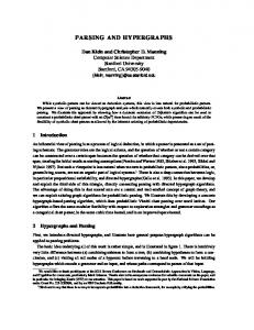
Figure 1: Representations of the different types of items used in parsing. (a) An inside edge item I(VP, 2, 5). (b) An outside edge item O(VP, 2, 5). (c) An inside derivation item: D(T VP , 2, 5). (d) An outside derivation item: G Q(TVP , 1, 2, {(N P, 2, n)}. The edges in boldface are frontier edges.
These deduction rules are “executed” within a generic agenda-driven algorithm, which constructs items in a prioritized fashion. The algorithm maintains an agenda (a priority queue of items), as well as a chart of items already processed. The fundamental operation of the algorithm is to pop the highest priority item φ from the agenda, put it into the chart with its current weight, and apply deduction rules to form any items which can be built by combining φ with items already in the chart. When the resulting items are either new or have a weight smaller than an item’s best score so far, they are put on the agenda with priority given by p(·). Because all antecedents must be constructed before a deduction rule is executed, we sometimes refer to particular conclusion item as “waiting” on another item before it can be built. 2.2
NP
NN
A∗
A∗ parsing (Klein and Manning, 2003) is an algorithm for computing the 1-best parse of a sentence. A∗ operates on items called inside edge items I(A, i, j), which represent the many possible inside derivations of an edge (A, i, j). Inside edge items are constructed according to the IN deduction rule of Table 1. This deduction rule constructs inside edge items in a bottom-up fashion, combining items representing smaller edges I(B, i, k) and I(C, k, j) with a grammar rule r = A → B C to form a larger item I(A, i, j). The weight of a newly constructed item is given by the sum of the weights of the antecedent items and the grammar rule r, and its priority is given by hypergraph search problems as shown in Klein and Manning (2001).
VP VP
NP
VP NN
G NP
NP
VP
s0 ... s2 s5 ... sn-1 (d)
VP
NP
VP
NN
s1 s2 s3 (a)
s4
s5
s0
s1 s2 s3 (b)
s4 s5
Figure 2: (a) An outside derivation item before expansion at the edge (VP, 1, 4). (b) A possible expansion of the item in (a) using the rule VP→ VP NN. Frontier edges are marked in boldface.
its weight plus a heuristic h(A, i, j). For consistent and admissible heuristics h(·), this deduction rule guarantees that when an inside edge item is removed from the agenda, its current weight is its true Viterbi inside score. The heuristic h controls the speed of the algorithm. It can be shown that an edge e satisfying β(e) + h(A, i, j) > β(G, 0, n) will never be removed from the agenda, allowing some edges to be safely pruned during parsing. The more closely h(e) approximates the Viterbi outside cost α(e), the more items are pruned. 2.3
KA∗
The use of inside edge items in A∗ exploits the optimal substructure property of derivations – since a best derivation of a larger edge is always composed of best derivations of smaller edges, it is only necessary to compute the best way of building a particular inside edge item. When finding k-best lists, this is no longer possible, since we are interested in suboptimal derivations. Thus, KA∗ , the k-best extension of A∗ , must search not in the space of inside edge items, but rather in the space of inside derivation items D(T A , i, j), which represent specific derivations of the edge (A, i, j) using tree T A . However, the number of inside derivation items is exponential in the length of the input sentence, and even with a very accurate heuristic, running A∗ directly in this space is not feasible. Fortunately, Pauls and Klein (2009) show that with a perfect heuristic, that is, h(e) = α(e) ∀e, A∗ search on inside derivation items will only remove items from the agenda that participate in the true k-best lists (up to ties). In order to compute this perfect heuristic, KA∗ makes use of outside edge items O(A, i, j) which represent the many possible derivations of G →
IN∗† : IN-D† : OUT-L† : OUT-R† : OUT-D∗ :
O(A, i, j) : w1 O(A, i, j) : w1 O(A, i, j) : w1
I(B, i, l) : w1 D(T B , i, l) : w2 I(B, i, l) : w2 I(B, i, l) : w2
I(C, l, j) : w2 D(T C , l, j) : w3 I(C, l, j) : w3 I(C, l, j) : w3
Q(TAG , i, j, F) : w1
I(B, i, l) : w2
I(C, l, j) : w3
w1 +w2 +wr +h(A,i,j)
−−−−−−−−−−−−−−→ w +w3 +wr +w1 −−2−−− −−−−−→ w +w3 +wr +w2 −−1−−− −−−−−→ w +w2 +wr +w3 −−1−−− −−−−−→ w1 +wr +w2 +w3 +β(F )
−−−−−−−−−−−−−−−→
I(A, i, j) : w1 + w2 + wr D(T A , i, j) : w2 + w3 + wr O(B, i, l) : w1 + w3 + wr O(C, l, j) : w1 + w2 + wr Q(TBG , i, l, FC ) : w1 + wr
Table 1: The deduction rules used in this paper. Here, r is the rule A → B C. A superscript * indicates that the rule is used in TKA∗ , and a superscript † indicates that the rule is used in KA∗ . In IN-D, the tree TA is rooted at (A, i, j) and has children T B and T C . P In OUT-D, the tree TBG is the tree TAG extended at (A, i, j) with rule r, FC is the list F with (C, l, j) prepended, and β(F) is e∈F β(e). Whenever the left child I(B, i, l) of an application of OUT-D represents a terminal, the next edge is removed from F and is used as the new point of expansion.
s1 . . . si A sj+1 . . . sn (see Figure 1(b)). Outside items are built using the OUT-L and OUT-R deduction rules shown in Table 1. OUTL and OUT-R combine, in a top-down fashion, an outside edge over a larger span and inside edge over a smaller span to form a new outside edge over a smaller span. Because these rules make reference to inside edge items I(A, i, j), these items must also be built using the IN deduction rules from 1-best A∗ . Outside edge items must thus wait until the necessary inside edge items have been built. The outside pass is initialized with the item O(G, 0, n) when the inside edge item I(G, 0, n) is popped from the agenda. Once we have started populating outside scores using the outside deductions, we can initiate a search on inside derivation items.3 These items are built bottom-up using the IN-D deduction rule. The crucial element of this rule is that derivation items for a particular edge wait until the exact outside score of that edge has been computed. The algorithm terminates when k derivation items rooted at (G, 0, n) have been popped from the agenda.
TKA∗
3
KA∗ efficiently explores the space of inside derivation items because it waits for the exact Viterbi outside cost before building each derivation item. However, these outside costs and associated deduction items are only auxiliary quantities used to guide the exploration of inside derivations: they allow KA∗ to prioritize currently constructed inside derivation items (i.e., constructed derivations of the goal) by their optimal completion costs. Outside costs are thus only necessary because we construct partial derivations bottomup; if we constructed partial derivations in a topdown fashion, all we would need to compute opti3
We stress that the order of computation is entirely specified by the deduction rules – we only speak about e.g. “initiating a search” as an appeal to intuition.
mal completion costs are Viterbi inside scores, and we could forget the outside pass. TKA∗ does exactly that. Inside edge items are constructed in the same way as KA∗ , but once the inside edge item I(G, 0, n) has been discovered, TKA∗ begins building partial derivations from the goal outwards. We replace the inside derivation items of KA∗ with outside derivation items, which represent trees rooted at the goal and expanding downwards. These items bottom out in a list of edges called the frontier edges. See Figure 1(d) for a graphical representation. When a frontier edge represents a single word in the input, i.e. is of the form (si , i, i + 1), we say that edge is complete. An outside derivation can be expanded by applying a rule to one of its incomplete frontier edges; see Figure 2. In the same way that inside derivation items wait on exact outside scores before being built, outside derivation items wait on the inside edge items of all frontier edges before they can be constructed. Although building derivations top-down obviates the need for a 1-best outside pass, it raises a new issue. When building derivations bottom-up, the only way to expand a particular partial inside derivation is to combine it with another partial inside derivation to build a bigger tree. In contrast, an outside derivation item can be expanded anywhere along its frontier. Naively building derivations top-down would lead to a prohibitively large number of expansion choices. We solve this issue by always expanding the left-most incomplete frontier edge of an outside derivation item. We show the deduction rule OUT-D which performs this deduction in Figure 1(d). We denote an outside derivation item as Q(TAG , i, j, F), where TAG is a tree rooted at the goal with left-most incomplete edge (A, i, j), and F is the list of incomplete frontier edges excluding (A, i, j), ordered from left to right. Whenever the application of this rule “completes” the left-
most edge, the next edge is removed from F and is used as the new point of expansion. Once all frontier edges are complete, the item represents a correctly scored derivation of the goal, explored in a pre-order traversal. 3.1
Correctness
It should be clear that expanding the left-most incomplete frontier edge first eventually explores the same set of derivations as expanding all frontier edges simultaneously. The only worry in fixing this canonical order is that we will somehow explore the Q items in an incorrect order, possibly building some complete derivation Q0C before a more optimal complete derivation QC . However, note that all items Q along the left-most construction of QC have priority equal to or better than any less optimal complete derivation Q0C . Therefore, when Q0C is enqueued, it will have lower priority than all Q; Q0C will therefore not be dequeued until all Q – and hence QC – have been built. Furthermore, it can be shown that the top-down expansion strategy maintains the same efficiency and optimality guarantees as KA∗ for all item types: for consistent heuristics h, the first k entirely complete outside derivation items are the true k-best derivations (modulo ties), and that only derivation items which participate in those k-best derivations will be removed from the queue (up to ties). 3.2
Implementation Details
Building derivations bottom-up is convenient from an indexing point of view: since larger derivations are built from smaller ones, it is not necessary to construct the larger derivation from scratch. Instead, one can simply construct a new tree whose children point to the old trees, saving both memory and CPU time. In order keep the same efficiency when building trees top-down, a slightly different data structure is necessary. We represent top-down derivations as a lazy list of expansions. The top node TGG is an empty list, and whenever we expand an outside derivation item Q(TAG , i, j, F) with a rule r = A → B C and split point l, the resulting derivation TBG is a new list item with (r, l) as the head data, and TAG as its tail. The tree can be reconstructed later by recursively reconstructing the parent, and adding the edges (B, i, l) and (C, l, j) as children of (A, i, j).
3.3
Advantages
Although our algorithm eliminates the 1-best outside pass of KA∗ , in practice, even for k = 104 , the 1-best inside pass remains the overwhelming bottleneck (Pauls and Klein, 2009), and our modifications leave that pass unchanged. However, we argue that our implementation is simpler to specify and implement. In terms of deduction rules, our algorithm eliminates the 2 outside deduction rules and replaces the IN-D rule with the OUT-D rule, bringing the total number of rules from four to two. The ease of specification translates directly into ease of implementation. In particular, if highquality heuristics are not available, it is often more efficient to implement the 1-best inside pass as an exhaustive dynamic program, as in Huang and Chiang (2005). In this case, one would only need to implement a single, agenda-based k-best extraction phase, instead of the 2 needed for KA∗ . 3.4
Performance
The contribution of this paper is theoretical, not empirical. We have argued that TKA∗ is simpler than TKA∗ , but we do not expect it to do any more or less work than KA∗ , modulo grammar specific optimizations. Therefore, we simply verify, like KA∗ , that the additional work of extracting k-best lists with TKA∗ is negligible compared to the time spent building 1-best inside edges. We examined the time spent building 100-best lists for the same experimental setup as Pauls and Klein (2009).4 On 100 sentences, our implementation of TKA∗ constructed 3.46 billion items, of which about 2% were outside derivation items. Our implementation of KA∗ constructed 3.41 billion edges, of which about 0.1% were outside edge items or inside derivation items. In other words, the cost of k-best extraction is dwarfed by the the 1-best inside edge computation in both cases. The reason for the slight performance advantage of KA∗ is that our implementation of KA∗ uses lazy optimizations discussed in Pauls and Klein (2009), and while such optimizations could easily be incorporated in TKA∗ , we have not yet done so in our implementation. 4
This setup used 3- and 6-round state-split grammars from Petrov et al. (2006), the former used to compute a heuristic for the latter, tested on sentences of length up to 25.
4
Conclusion
We have presented TKA∗ , a simplification to the KA∗ algorithm. Our algorithm collapses the 1best outside and bottom-up derivation passes of KA∗ into a single, top-down pass without sacrificing efficiency or optimality. This reduces the number of non base-case deduction rules, making TKA∗ easier both to specify and implement.
Acknowledgements This project is funded in part by the NSF under grant 0643742 and an NSERC Postgraduate Fellowship.
References Liang Huang and David Chiang. 2005. Better k-best parsing. In Proceedings of the International Workshop on Parsing Technologies (IWPT), pages 53–64. V´ıctor M. Jim´enez and Andr´es Marzal. 2000. Computation of the n best parse trees for weighted and stochastic context-free grammars. In Proceedings of the Joint IAPR International Workshops on Advances in Pattern Recognition, pages 183–192, London, UK. Springer-Verlag. Dan Klein and Christopher D. Manning. 2001. Parsing and hypergraphs. In Proceedings of the International Workshop on Parsing Technologies (IWPT), pages 123–134. Dan Klein and Christopher D. Manning. 2003. A* parsing: Fast exact Viterbi parse selection. In Proceedings of the Human Language Technology Conference and the North American Association for Computational Linguistics (HLT-NAACL), pages 119–126. Mark-Jan Nederhof. 2003. Weighted deductive parsing and Knuth’s algorithm. Computationl Linguistics, 29(1):135–143. Adam Pauls and Dan Klein. 2009. K-best A* parsing. In Proccedings of the Association for Computational Linguistics (ACL). Slav Petrov, Leon Barrett, Romain Thibaux, and Dan Klein. 2006. Learning accurate, compact, and interpretable tree annotation. In Proccedings of the Association for Computational Linguistics (ACL). Stuart M. Shieber, Yves Schabes, and Fernando C. N. Pereira. 1995. Principles and implementation of deductive parsing. Journal of Logic Programming, 24:3–36. Frank K. Soong and Eng-Fong Huang. 1991. A treetrellis based fast search for finding the n best sentence hypotheses in continuous speech recognition. In Proceedings of the Workshop on Speech and Natural Language.