December 11, 2015. CMU-ISR-15-108. Institute for Software ... done in the field of topic modeling in social media data, this work incorporates various ..... of hashtags were associated with advertising campaigns or related to news. Figure 4.2.
Topic Modeling in Large Scale Social Network Data Aman Ahuja*, Wei Wei, Kathleen M. Carley December 11, 2015 CMU-ISR-15-108
Institute for Software Research School of Computer Science Carnegie Mellon University Pittsburgh, PA 15213
Center for Computational Analysis of Social and Organizational Systems: CASOS technical report.
This work is an independent project that leverages the work that was in part supported by the Office of Naval Research N00014140737 with support from CMU for social media analytics by Dr. Carley and Mr. Wei. Additional support for this project was provided by the Center for Computational Analysis of Social and Organizational Systems (CASOS) at CMU. The views and conclusions contained in this document are those of the authors and should not be interpreted as representing the official policies, either expressed or implied, of the Office of Naval Rsearch or the U.S. Government
*Undergraduate student, BITS Pilani – K.K. Birla Goa Campus, India
Keywords: Topic Modeling, Social Network Analysis, Probabalistic Graphical Models
Abstract The growing popularity of social media such as Twitter and Facebook has made these websites an important source of information. The large amount of data available on these platforms presents new opportunities for mining information about the real world. Because of its widespread usage, a lot of useful information can be extracted from the text available on these social media platforms. It can be used to infer important aspects about the users of these services and about the things happening in their surroundings. This work proposes generative probabalistic models to identify latent topics and sentiments in social media data, mainly Twitter. In contrast to the majority of earlier work done in the field of topic modeling in social media data, this work incorporates various special characteristics of this data- mainly the short-length nature and special tokens like hashtags. The models proposed in work were compared qualitatively and quantitatively against several baseline models for evaluation. Experimental results suggest several improvements over the existing baseline techniques.
1
List of Figures 4.1 4.2 4.3 4.4
Plate notation of SMTM . . . . . . . . . . . Topic-category distribution with K = 60 . . Perplexity comparison of SMTM with LDA . Running time per iteration for SMTM . . .
5.1 5.2 5.3 5.4
Plate notation of SMSTM . . . . . . . . . . . . Perplexity comparison of SMSTM with JST . . Sentiment accuracy comparison of SMSTM with Running time per iteration for SMSTM . . . . .
2
. . . .
. . . .
. . . .
. . . .
. . . .
. . . .
. . . .
. . . .
. . . .
. . . .
. . . .
. . . .
. . . .
. . . .
. . . .
. . . .
10 14 15 16
. . . . . . JST . . .
. . . .
. . . .
. . . .
. . . .
. . . .
. . . .
. . . .
. . . .
. . . .
. . . .
. . . .
17 23 23 24
Contents List of Figures
2
Contents
3
1 Introduction
5
2 Related Work 2.1 Topic Modeling . . . . . . . . . . . . . . . . . . . . . . . . . . . . . . . . 2.2 Sentiment Analysis . . . . . . . . . . . . . . . . . . . . . . . . . . . . . . 2.3 Modeling Social Media Data . . . . . . . . . . . . . . . . . . . . . . . . .
6 6 6 6
3 Dataset 3.1 Twitter Dataset . . . . . . . . . . . . . . . . . . . . . . . . . . . . . . . . 3.1.1 Special characteristics of Twitter ”tweets” . . . . . . . . . . . . . 3.2 Preprocessing . . . . . . . . . . . . . . . . . . . . . . . . . . . . . . . . .
8 8 8 8
4 SMTM: Social Media Topic Model 4.1 Model Description . . . . . . . . . 4.2 Generative Process . . . . . . . . . 4.3 Inference . . . . . . . . . . . . . . . 4.4 Experimental Results . . . . . . . . 4.4.1 Experimental Setup . . . . . 4.4.2 Qualitative Results . . . . . 4.4.3 Quantitative Results . . . . 4.4.4 Running time . . . . . . . . 4.5 Conclusion . . . . . . . . . . . . . .
. . . . . . . . .
10 10 11 11 13 13 13 14 15 16
. . . . . . . . . .
. . . . . . . . . .
17 17 18 18 19 21 21 21 22 24 24
6 Conclusion 6.1 Summary of Contributions . . . . . . . . . . . . . . . . . . . . . . . . . 6.2 Scope . . . . . . . . . . . . . . . . . . . . . . . . . . . . . . . . . . . . 6.3 General strengths and weaknesses of Bayesian models in topic modeling 6.4 Directions for Future Work . . . . . . . . . . . . . . . . . . . . . . . . .
. . . .
25 25 25 25 26
. . . . . . . . .
. . . . . . . . .
. . . . . . . . .
. . . . . . . . .
. . . . . . . . .
. . . . . . . . .
. . . . . . . . .
5 SMSTM: Social Media Sentiment Topic Model 5.1 Model Description . . . . . . . . . . . . . . . . 5.2 Generative Process . . . . . . . . . . . . . . . . 5.3 Inference . . . . . . . . . . . . . . . . . . . . . . 5.4 Sentiment Lexicon . . . . . . . . . . . . . . . . 5.5 Experimental Results . . . . . . . . . . . . . . . 5.5.1 Experimental Setup . . . . . . . . . . . . 5.5.2 Qualitative Results . . . . . . . . . . . . 5.5.3 Quantitative Results . . . . . . . . . . . 5.5.4 Running time . . . . . . . . . . . . . . . 5.6 Conclusion . . . . . . . . . . . . . . . . . . . . .
3
. . . . . . . . .
. . . . . . . . . .
. . . . . . . . .
. . . . . . . . . .
. . . . . . . . .
. . . . . . . . . .
. . . . . . . . .
. . . . . . . . . .
. . . . . . . . .
. . . . . . . . . .
. . . . . . . . .
. . . . . . . . . .
. . . . . . . . .
. . . . . . . . . .
. . . . . . . . .
. . . . . . . . . .
. . . . . . . . .
. . . . . . . . . .
. . . . . . . . .
. . . . . . . . . .
. . . . . . . . .
. . . . . . . . . .
. . . . . . . . .
. . . . . . . . . .
. . . . . . . . .
Bibliography
27
Appendices
29
A Derivation of Gibbs Sampling Equation for SMTM
30
B Derivation of Gibbs Sampling Equation for SMSTM
32
4
1. Introduction The rapid growth of Internet in recent years has led to the growth of several social media websites like Twitter and Facebook in the recent years. People use these platforms to post about different aspects of their life and about the things happening in their surroundings. Using such platforms, people with similar interests can connect with each-other, create groups and share content such as messages, media with each other. Because of their increasing use and the vast quantity of data, this data can be used in several ways to gather information about the world, such as trending topics, breaking news and popular events. In contrast to other forms of media such as newspaper, the text in the posts found on these websites is usually short in length, and concentrated on a much narrower selection of topics. Another interesting feature of social media data is the use of special tokens such as hashtags, that contain unique semantic meanings that are not captured by other ordinary words. Also, since a majority of people these days use handheld devices like mobile phones to access these services, a lot of data available on these platforms is geotagged. This information can be useful to determine various location-specific aspects around the world. This thesis is focused on topic modeling as a means to discover latent topics in social media data, mainly Twitter. Several topic modeling techniques have been proposed in the recent years. Most of these models are based on the Latent Dirichlet Allocation [1]. But whether these techniques can be used to model social media text, which differs from other forms of text in variety of ways has not been well studied. In this work, we address the challenge of modeling social media text using Bayesian graphical models that take into account the special characteristics of the social media text, such as their short-length nature and special tokens such as hashtags. We also present both qualitative and quantitative evaluation of the proposed models against several baseline models. The subsequent chapters are organized as follows: • Chapter 2 gives an overview of the several topic modeling techniques that have been proposed so far. • Chapter 3 describes the Twitter dataset that was used to evaluate the models presented in this work • Chapter 4 presents a generative model, namely SMTM(Social Media Topic Model ) to discover latent topics in social media data. This model characterizes both words and hashtags separately, and takes into account the short-length nature of social media posts. • Chapter 5 presents a sentiment topic model, namely SMSTM(Social Media Sentiment Topic Model ). This model is an extension of SMTM, but also incorporates the sentiment. • Chapter 6 outlines the major contributions of the work presented in this work, which is followed by the outline directions for future work. 5
2. Related Work This chapter presents an overview of the several previous works that are related to this thesis. The focus here will be on 3 main categories- topic modeling, sentiment analysis and modeling social media data.
2.1. Topic Modeling The success of topic modeling in recent years has gained a lot of interest among the research community. A topic model is a probabalistic model that can be used to discover latent topics in a corpus of documents. One of the earliest technique in the field of topic modeling was the probabalistic Latent Semantic Indexing (pLSI) proposed by Hoffman [2]that models a document as a mixture of topics. pLSI models each document as a mixture over topics, but there is no generative process for determining the document-topic distribution, which leads to problems while assigning probabilities to documents outside the training set. Most of the recent research in the field of topic modeling is based on the Latent Dirichlet Allocation [1] proposed by Blei. LDA overcomes the shortcomings of pLSI by modeling each document as a mixture over topics, and each topic as a mixture over words.
2.2. Sentiment Analysis Sentiment analysis of social media data remains a key area of research. A lot of techniques ([3], [4]) have been proposed to detect sentiment polarity of Twitter messages. A majority of work in the field of sentiment analysis for Twitter data aims to classify the polarity of individual messages, and not of the topics as a whole. Unlike these work, we focus on learning the latent representations of the sentiment topic as well as the documents instead of predicting the sentiment label of the individual messages. One of the earliest work that incorporates sentiment associated with topics using a generative model model was the Joint Sentiment Topic(JST) model [5]. JST models each each document as a mixture over topics and sentiments. The prior sentiment knowledge about different words is used in the initialization step while assigning polarity to different words in each document. In this way, JST models the documents as a mixture of positive and negative topics. More recently, [6] proposed ASUM, that assigns topic and sentiment at the sentence level, unlike JST that assigns topic and sentiment at the word level. But since ASUM generates topics from sentiment, it finds senti-aspects, and does not perform reasonably well to find positive and negative aspects of each topic. Also, when applied to social media data, both JST and ASUM do not treat words and hashtags separately.
2.3. Modeling Social Media Data A number of techniques based on LDA have been proposed for social media data. The Author-Topic model proposed in [7] that can be used to determine the topic distributions
6
of various authors in the dataset. [8] discussed the application of the this model to Twitter data. But this model generally does not fit well in case of social media data where the documents are usually short in length, and belong to a single topic. [9] takes into account this property, and proposed Twitter-LDA model, that assigns topics at the tweet level, but does not treat both words and hashtags separately. Apart from the growing usage of topic modeling techniques for text, some of the recent work also aims to to use these techniques for other forms of data, such as the network dataset in social networks. The SSN-LDA model [10] is one such work that tries to model communities in social networks using a generative model. The SMTM and SMSTM models proposed in this work are largely inspired by TwitterLDA model and ASUM on the fact that topics are assigned at the document level. In addition, SMTM and SMSTM treat both words and hashtags separately. Also, SMSTM aims to find the positive and negative aspects of each topic, unlike ASUM, that discovers positive and negative topics.
7
3. Dataset This chapter gives details about the dataset used to evaluate the models presented in this work.
3.1. Twitter Dataset To evaluate the models, I used Twitter dataset collected using the Twitter Streaming API 1 . When collecting the data, the geo-region bounding that was selected roughly covered the entire area of USA. This dataset was then preprocessed before it could be used for the models described in this thesis. In total, there were around 2.4 million tweets collected within a 30-day time period from May 1, 2011 to May 31, 2011. Table 3.1: Dataset Statistics
Number of users(U) Number or unique words(W) Number of unique hashtags(H)
11509 557318 100445
3.1.1. Special characteristics of Twitter ”tweets” In contrast to other forms of text, the text in tweets is relatively short in length, restricted by the limit on the number of characters, which is 140 in case of Twitter. Because of this, the text also contains a lot of abbreviations, so that the information can be conveyed with limited number of characters. It is observed that tweets generally contain a lot of mis-spelled words also. This makes topic mining and text analysis using Twitter data a challenging task. Hashtags: A hashtag is a meta tag frequently used in social media posts, that can be used to link the post to a specific theme or topic. It is generally observed that popular events and topics are characterized by common hashtags, and it makes it easier to find the posts related to that topic. For example, people might use the tag #Halloween, if they tweet about something that is related to Halloween festival.
3.2. Preprocessing All the tweets used to evaluate the models were first preprocessed to remove the noisy and irrelevant words. The various steps involved in preprocessing stage were as follows: • Tokenization of emoticons: Since emoticons are useful in sentiment analysis, the first step was to replace all the valid emoticons with different tokens, so that they were not lost while removing the punctuation marks. 1
https://dev.twitter.com/streaming/overview
8
• Conversion to lowercase: All the letters in the dataset were converted to lowercase in order to prevent duplicates, and preserve the semantic meaning of same words that had different case letters. • URL and co-mentions removal: The third step was the removal of URLs and co-mentions, so that the text contains only meaningful words. • Stop word removal: Since stop words like for, the do not convey any meaning and are not topic-specific words, these words were also removed. • Removing infrequent words: Since words that occur very frequently in the corpus (less than 2 times) are more likely to be mis-spelled words, all such words from the dataset. • Restoring emoticons and tokenization: The final step of the preprocessing stage involved replacing the emoticon tokens assigned in step-1 with the original emoticons. This was followed by tokenization of all the words and tags. Tokenization of all the tweets in preprocessing stage improves performance, since we do not need to tokenize the entire corpus during run-time.
9
4. SMTM: Social Media Topic Model Given the growing usage of social media services, it has become increasingly important to determine what are the key topics that are dominant on these platforms. This can give an insight about the major things happening around in the world such as major events, disasters, etc. This chapter proposes SMTM(Social Media Topic Model )- a probabalistic model to discover latent topics in social media data. In contrast to other previously defined models, SMTM takes into account special characteristics of social media data, which distinguishes it from other models.
4.1. Model Description SMTM models the generative process of social media posts that contain both words and hashtags. In contrast to LDA, SMTM treats both words and hashtags separately and gives a topic-word distribution φ and topic-hashtags distribution η for each topic. Also, since social media posts are generally short in length (eg., 140 characters in Twitter ), it is highly likely that all words in a tweet belong to the same topic. SMTM takes into account this assumption, and assigns topic at the document level for each social media post. It models each user u as a mixture over topics (or interests), and then generates the topic z for each post by the user based on the user-topic distribution θu . It then assigns this topic to all the words and hashtags in the post. It is also observed that some topics (eg., those related to a popular event) contain a higher proportion of hashtags than other topics. SMTM also incorporates this fact using a dependency from the topic z to the category of the word token c. The value of this category variable c determines whether a token is a word or a #tag.
η
φK
β
K
w α
θ
φS
β
ϵ
z
α c
N
η
S
K
z
w
s
c
θ N
T
π
K
Figure 4.1: Plate notation of SMTM
10
T U
U
γ
ϵ K
λ
ΨK
π
γ S
K
4.2. Generative Process The overall generative process of SMTM can be described as follows: • For each topic k, – Draw topic-word distribution φk ∼Dirichlet(β) – Draw topic-tag distribution ηk ∼Dirichlet(�) – Draw topic-category distribution πk ∼Dirichlet(γ) • For each user u, draw user-topic distribution θu ∼Dirichlet(α) • For each post t by user u, choose a topic zut ∼M ultinomial(θu ) • For each token n in the post t by user u, – Choose a category cutn ∼Bernoulli(πzut ) – Draw a word/tag wutn as follows: ( M ultinomial(φzut ), if cutn = 1 wutn ∼ M ultinomial(ηzut ), if cutn = 0
4.3. Inference The joint probability distribution of SMTM can be given by he following equation: P (Z, W , C,θ, φ, η, π|α, β, �, γ) =
K Y
K Y
P (φi1 |β)
i1 =1
i2 =1
T Y
N Y
t=1
P (Zut |θu )
P (ηi2 |�)
K Y i3 =1
P (πi3 |γ)
U Y
P (θu |α)
u=1
(4.1)
P (Cutn |πZut )P (Wutn |Cutn , φZutn , ηZutn )
n=1
To infer the latent variable z, we use the collapsed Gibbs sampling technique described in [11]. The model parameters θ, π, φ and η were first integrated out, which gives the following distribution: P (Z, W , C|α, β, �, γ) = P QK U i Y Γ( K i=1 αi ) i=1 Γ(Nu + αi ) QK PK i i=1 Γ(αi ) Γ( i=1 Nu + αi ) u=1 QW P K i1 Y Γ( W r=1 Γ(Mwr + βr ) r=1 βr ) QW PW i1 r=1 Γ(βr ) Γ( r=1 Mwr + βr ) i1 =1 QH P K i2 Y Γ( H r=1 Γ(Mhr + �r ) r=1 �r ) QH PH i2 r=1 Γ(�r ) Γ( r=1 Mhr + �r ) i2 =1 P Q K Y Γ( 1r=0 γr ) 1r=0 Γ(Cri + γr ) Q1 P1 i r=0 Γ(γr ) Γ( r=0 Cr + γr ) i3 =1 11
(4.2)
The only variables left after integration are z, w and c. Since w and c are observed variables, we only sample z for each post (u, t) since it is the only latent variable left after integration. It is done according to the following equation: N k,−ut + αk P (zut = k|Z−ut , C, W , α, β, γ, �) ∝ PK u i,−ut + αi i=1 Nu Q Qnw,r −1 ut (Mwk,−ut + βr + j) j=0 r∈Wut r Qnw,(.) P −1 k,−ut ut (( W + βr ) + j) j=0 r=1 Mwr Q Qnh,r ut −1 (Mhk,−ut + �r + j) j=0 r∈Hut r h,(.) Qnut −1 PH + �r ) + j) (( r=1 Mhk,−ut j=0 r r,(.) Q1 Qnut −1 k,−ut (Cr + γr + j) j=0 r=0 (.),(.) Qnut −1 P1 (( r=0 Crk,−ut + γr ) + j) j=0
(4.3)
After sampling, the model parameters can be recovered using the following equations: θuk
k + αk Nu,(.)
= PK
i=1
i Nu,(.) + αi
M k + βr φrk = PW wr k r=1 Mwr + βr
(4.5)
M k + �r ηkr = PH hr k r=1 Mhr + �r
(4.6)
C k + γc πkc = P1 c k r=0 Cr + γr
(4.7)
The definitions of all the equations is given in Table 4.1 and Table 4.2. U T N K W H z w c θ φ η π α β � γ λ
(4.4)
the number of users the number of posts/tweets the number of tokens(words and hashtags) in each post the number of topics the size of word vocabulary the size of hashtag vocabulary topic word category (word or hashtag) user-topic distribution topic-word distribution topic-hashtag distribution topic-token category distribution Dirichlet prior vector for θ Dirichlet prior vector for φ Dirichlet prior vector for η Dirichlet prior vector for π, πs Dirichlet prior vector for ψ
Table 4.1: Notations: SMTM
12
Nuk Mwk r Mhkr Crk Wut Hut nx,r u,t
number of tweets by user u that occurred in topic k number of occurrences of rth word from word vocabulary in topic k number of occurrences of rth hashtag from hashtag vocabulary in topic k number of occurrences of tokens from category r in topic k set of unique words in the post (u,t) set of unique hashtags in the post (u,t) number of occurrences of rth token from vocabulary x in post (u,t)
Table 4.2: Auxiliary Notations: SMTM 1
4.4. Experimental Results 4.4.1. Experimental Setup In order to evaluate SMTM, we first need to input the values of the hyperparameters α, β, γ and �. These hyperparameters serve as a priori for the model. We used symmetric values for all the hyperparameters, which were derived experimentally. Specifically, we set α = 1, β = 0.05, � = 0.05 and γ = 5. The model was run for 800 iterations, using different values for the number of topics, K.
4.4.2. Qualitative Results In order to demonstrate the qualitative results, two topics from the results were selected and their topi 10 words and hashtags were picked based on the corresponding values of the topic-word distribution φ and topic-tag distribution η. These results are presented in Table 4.3. As it is evident from the results shown in Table 4.3, first topic contains words and tags that are related to a particular event, i.e., the death of Osama Bin Laden, since the Twitter dataset was from May, 2011 (the same time when US assassinated Osama Bin Laden). The second topic mostly has words related to food, particularly good food as it contains words like ”eat”, ”good”, ”food”, etc. These words are supported by corresponding hashtags like ”#fattweet”, ”#yum”, ”#hungry”, etc. Topic-category distribution: We compare the value of the parameter π for different topics and examine the corresponding words and hashtags for each topic. It is observed that for a majority of topics, the ratio πk,0 : πk,1 of number of words to the number of hashtags assigned to that topic is around 0.25. Some topics have a high distribution of hashtags as compared to other topics. After examining the corresponding words and hashtags for these topics, it was observed that most of the topics with higher proportion 1
For all the terms shown in the equations, • (-u,t) denotes that the term excludes the current post (u,t) • for any dimension d, (.) denotes that the term is not limited to the specific value of d
13
of hashtags were associated with advertising campaigns or related to news. Figure 4.2 shows the values of πk,0 (#tags) and πk,1 (words) for all the topics when K = 60.
Figure 4.2: Topic-category distribution with K = 60
4.4.3. Quantitative Results To compare SMTM quantitatively with other models, we choose LDA as the baseline model and compare the perplexity of both the models, which is a commonly used criterion for evaluating topic models. The perplexity of a model for a test set containing M documents is defined as: ) ( P − M log p(w ) d d=1 P erp(Dtest ) = exp (4.8) P M d=1 Nd Since we are interested in comparing the perplexity of SMTM with LDA, the exponent term can be ignored. Th perplexity of SMTM can be calculated as per the following T1:Words bin laden obama osama news dead death world killed man
T1:#tags #caseyanthonytrial #osama #syria #news #obama #pakistan #binladen #usa #osamabinladen #dead
T2:Words eat good food chicken :) icecream eating breakfast cheese drink
T2:#tags #fattweet #win #yum #yummy #hungrytweet #hungry #munchies #love #delicious #ny
Table 4.3: Sample words and hashtags for 2 different topics obtained using SMTM 14
equation: SM T M )= P erp(Dtest
PU
u=1
1 PT
t=1
U X T X
Nut
u=1 t=1
log
K X k=1
ut
θu,k
Nw X
πk,1 φk,n
n=1
(4.9)
Nhut
+
X
πk,0 ηk,n
��
n=1
As described in [1], a lower perplexity score indicates better predictive performance of the model. A high likelihood value indicates that model has a better predictive accuracy. Since perplexity is the negative log of the likelihood p(w), a model with lower perplexity is more likely to have a better predictive performance. The perplexity of SMTM was compared with that of LDA, using different values of K ranging from 5 to 100. The perplexity comparison is shown in Figure 4.3. The lower perplexity of SMTM against LDA indicates that SMTM has a better predictive performance in case of social media data.
Figure 4.3: Perplexity comparison of SMTM with LDA
4.4.4. Running time We now show the running time per Gibbs sampling iteration for the corpus containing 2.38 million tweets. It is observed that the running time increases almost linearly as the number of topics K increases. This is shown in Figure 4.4. This is because as the number of topics increases, for each post (u, t), the number of times that we need to calculate the marginal probability of latent variables also increases.
15
Figure 4.4: Running time per iteration for SMTM
4.5. Conclusion In this chapter, we presented a novel topic model to discover latent topics in social media dataset. One key characteristic of this model was that it is particularly designed for social media text, which differs from other forms of text in a variety of ways. We evaluated our model on Twitter dataset, although since the structure of data on different social meda platforms is similar, we believe that the model can perform reasonably well on other datasets also. We compared our model with the existing baseline model and found that it outperforms the baseline model.
16
5. SMSTM: Social Media Sentiment Topic Model Chapter 4 introduced a novel method to discover latent topics from social media data. In addition to discovering topics, it is equally important to determine the sentiments associated with the topics. It can be useful in determining whether a topic is good or bad, based on the sentiment polarity associated with topic. For example, a topic associated with a natural disaster like tornado has negative sentiment, but a topic that describes nightlife and holidays has positive polarity. Also, there are some topics that have both positive and negative aspects. For example, topic associated with Presidential elections in the United States can have both positive and negative aspects associated with different candidates contesting for he elections. To tackle this problem, we introduce SMSTM(Social Media Sentiment Topic Model ), that can discover topics and their sentiment from a corpus containing social media data.
5.1. Model Description SMSTM is a generative model that can discover latent topics and sentiments in social media data. This model is an extension of SMTM, but it also incorporates the sentiment associated with the topics. The graphical model for SMSTM is shown in Figure 5.1. In addition to all the other variables in SMTM, SMSTM has a sentiment variable s at the document level, which is the sentiment polarity of the document. This is drawn from the sentiment distribution ψz of the topic z associated with the document, which can determine the sentiment associated the topic. For each token in the document (u, t), after determining the category (word or hashtag) of the token, it is drawn from the respective topic-sentiment-word distribution φk,s or ηk,s based on the value of the variable c. The prior sentiment polarity of words can be incorporated into SMSTM in the values of the hyperparameters β and � based on the assumption that since a word with positive sentiment polarity is more likely to be in a positive sentiment topic. Intuitively, the model can be described as follows: whenever a user u, decides to write a post t, he first decides the topic zut of the post based on his interest distribution θu . He then decides the sentiment sut and the type(word or hashtag) of the tokens in the post. Finally, he generates the tokens wutn based on the topic, sentiment and category of the tokens.
η
φK
β
S
w α
θ
z
α c
N
φS
β
ϵ K
η
S
K
z
w
s
c
θ N
T
π
K
T U
U
γ
ϵ K
λ
ΨK
π
γ S
K
Figure 5.1: Plate notation of SMSTM 17
5.2. Generative Process The generative process of SMSTM can be described as follows: • For each topic k, – Draw topic-sentiment distribution ψk ∼Dirichlet(λ) – For each sentiment s, ∗ Draw topic-sentiment-category distribution πk,s ∼Dirichlet(γ) ∗ Draw topic-sentiment-word distribution φk,s ∼Dirichlet(βs ) ∗ Draw topic-sentiment-hashtag distribution ηk,s ∼Dirichlet(�s ) • For each user u, – Draw user-topic distribution θu ∼Dirichlet(α) – For each post t by the user, ∗ Choose a topic zut ∼M ultinomial(θu ) ∗ Choose a sentiment sut ∼M ultinomial(ψzut ) ∗ For each token n in the post (u, t), · Choose a category cutn ∼M ultinomial(πzut ,sut ) · Draw a word/hashtag as follows: ( M ultinomial(φzut ,sut ), if cutn = 1 wutn ∼ M ultinomial(ηzut ,sut ), if cutn = 0
5.3. Inference The joint probability distribution for SMSTM can be given as: P (Z, S, W , C, θ, ψ, π, φ, η|α, β, �, γ, λ) =
K Y S Y
P (πi3 ,s |γs )
i3 =1 s=1 K Y S Y
u=1 N Y
P (φi1 ,s |βs )
P (θu |α)
P (ψi4 |λ)
i4 =1
i1 =1 s=1 U Y
K Y
K Y S Y
P (ηi2 ,s |�s )
i2 =1 s=1 T Y
P (zut |θu )P (sut |ψzut )
t=1
P (Cutn |πzut ,sut )P (Wutn |Cutn , φzut ,sut , ηzut ,sut )
n=1
(5.1) Similar to SMTM, the inference in SMSTM is also done using collapsed Gibbs sampling. All the model parameters θ, ψ, φ, η and π are integrated out easily because of the Dirichlet-Multinomial conjugacy. In addition to the topic variable z, SMSTM has one
18
additional latent variable s that needs to be sampled for each tweet (u, t). For each post (u, t), this sampling can be done as per the following equation: P (zut = k, sut = p|Z−ut , S−ut , C, W , α, β, �, γ, λ) ∝ k,−ut Nu,(.) + αk
Lk,p,−ut + λp P 1 i,−ut k,s,−ut + λ s s=0 L i=1 Nu,(.) + αi Q Qnw,r ut −1 (Mwk,p,−ut + βr + j) j=0 r∈Wut r w,(.) Qnut −1 PW (( r=1 Mwk,p,−ut + βr ) + j) r j=0 h,r Qnut −1 k,p,−ut Q (Mhr + �r + j) j=0 r∈Hut Qnh,(.) P k,p,−ut ut −1 + �r ) + j) (( H j=0 r=1 Mhr Q1 Qnr,(.) ut −1 (Crk,p,−ut + γr + j) j=0 r=0 (.),(.) Qnut −1 P1 (( r=0 Crk,p,−ut + γr ) + j) j=0 PK
(5.2)
The model parameters θ, ψ, φ, η and π can then be calculated as per the following equations: k + αk Nu,(.) (5.3) θuk = PK i N + α i i=1 u,(.) M k,p + βp,r φrk,p = PW wr k,p r=1 Mwr + βp,r r ηk,p
Mhk,p + �p,r r
= PH
k,p r=1 Mhr + �p,r
C k,p + γc c πk,p = P1 c k,p r=0 Cr + γr ψkp
Lk,p (.) + λp
= P1
s=0
Lk,s (.) + λs
(5.4)
(5.5) (5.6)
(5.7)
(All the notations are described in Table 5.1 and Table 5.2)
5.4. Sentiment Lexicon To incorporate the prior sentiment polarity of words in SMSTM, Vader sentiment lexicon[12] was used. This choice was made based on the fact that Vader is specifically designed for words that frequently occur in social media posts, particularly Twitter and is highly optimized for such datasets. Also, a lot of these commonly occurring polar words are present only in Vader, and cannot be found in other sentiment lexicons like the MPQA subjectivity corpus[14] and SentiWordnet[13]. Since in our experiments, we consider only positive and negative sentiments, we separate out the positive and negative sentiment words from Vader based on their score. After this, the sentiment lexicon had 3300 positive sentiment words and 4100 negative sentiment words. 19
U T N K S W H z w c s θ φ η π ψ α βs �s γs λ
the number of users the number of posts/tweets the number of tokens(words and hashtags) in each post the number of topics the number of sentiments the size of word vocabulary the size of hashtag vocabulary topic word category (word or hashtag) sentiment user-topic distribution topic-word distribution topic-hashtag distribution topic-token category distribution topic-sentiment distribution Dirichlet prior vector for θ Dirichlet prior vector for φs Dircihlet prior vector for ηs Dirichlet prior vector for πs Dirichlet prior vector for ψ
Table 5.1: Notations: SMSTM
k Nu,t Wut Hut nx,r u,t Mwk,p r Mhk,p r Crk,p Lk,p
number of times tweet (u, t) has occurred in topic k set of unique words in the post (u,t) set of unique hashtags in the post (u,t) number of occurrences of rth token from vocabulary x in post (u,t) number of occurrences of rth word from word vocabulary in topic k with polarity p number of occurrences of rth hashtag from hashtag vocabulary in topic k with polarity p number of occurrences of tokens from category r in topic k with polarity p total number of posts that are assigned topic k and p
Table 5.2: Auxiliary Notations
20
5.5. Experimental Results 5.5.1. Experimental Setup To evaluate SMSTM, the same Twitter dataset as the one used for SMTM was used ( 2.4 million tweets). The number of sentiments (S ) was set to 2, since we were only interested in positive and negative topics. The hyperparameters α, λ and γ were assigned symmetric values, which were determined experimentally. These were α = 1, λ = 5 and γ = 5. As described earlier, the prior sentiment knowledge in SMSTM is incorporated by making β and � unsymmetrical vectors. Since hashtags are not proper words that can be found in the english vocabulary, the hyperparameter � was assigned symmetric value equal to 0.05. For each word r that was present in the sentiment lexicon, the value of β was assigned as follows: ( 0.09, if polarity(r)=s βrs = 0.01, if polarity(r) 6= s For all the other words r whose prior sentiment knowledge was not known, a symmetric βr was assigned which was equal to 0.05. During the initialization step for each post (u, t), the number of positive words(pos) and negative words(neg) was calculated by comparing each word in post (u, t) against the sentiment lexicon. After this, the sentiment sut was assigned as follows: if pos>neg 1, if pos