Topics in semantic association - Semantic Scholar

Topics in semantic association Thomas L. Griffiths Department of Cognitive and Linguistic Sciences Brown University

Mark Steyvers Department of Cognitive Sciences University of California, Irvine

Joshua B. Tenenbaum Department of Brain and Cognitive Sciences Massachusetts Institute of Technology Abstract Learning and using language requires retrieving concepts from memory in response to an ongoing stream of information. The human memory system solves this problem by using the gist of a sentence, conversation, or document to predict related concepts and disambiguate words. Two approaches to representing gist have dominated research on semantic representation: semantic networks and semantic spaces. We take a step back from these approaches, and analyze the abstract computational problem underlying the extraction and use of gist, formulating this problem in statistical terms. This analysis allows us to explore a novel approach to semantic representation, in which words are represented using a set of probabilistic topics. The topic model performs well in predicting word association, free recall, and the senses of words, and provides a foundation for developing richer statistical models of language.

Learning, speaking, and understanding language all require solving a challenging computational problem: retrieving a variety of concepts from memory in response to an ongoing stream of information. The human memory system solves this problem by using the semantic context – the gist of a sentence, conversation, or document – to predict related concepts and disambiguate words. Online processing of sentences can be facilitated by predicting which concepts are likely to be relevant before they are needed. For example, if the word BANK appears in a sentence, it might become more likely that words like FEDERAL and RESERVE would also appear in that sentence, and this information could be used to initiate retrieval of the information related to these words. This pre-

This work was supported by a grant from the NTT Communication Sciences Laboratory. While completing this work, TLG was supported by a Stanford Graduate Fellowship, and JBT by the Paul E. Newton chair. We thank Touchstone Applied Sciences, Tom Landauer, and Darrell Laham for making the TASA corpus available, and for their thoughts on these topics.

TOPICS IN SEMANTIC ASSOCIATION

2 Topic

(a)

(b) STREAM

MEADOW

(c)

RESERVE FEDERAL BANK MONEY LOANS COMMERCIAL

BANK

RESERVE

FEDERAL

DEPOSITS STREAM RIVER DEEP FIELD MEADOW WOODS GASOLINE PETROLEUM CRUDE DRILL

OIL

1 2 3 BANK COMMERCIAL CRUDE DEEP DEPOSITS DRILL FEDERAL FIELD GASOLINE LOANS MEADOW MONEY OIL PETROLEUM RESERVE RIVER STREAM WOODS

MONEY OIL STREAM BANK PETROLEUM RIVER FEDERAL GASOLINE BANK RESERVE CRUDE DEEP LOANS COMMERCIAL WOODS DEPOSITS DEPOSITS FIELD COMMERCIAL RIVER MONEY DEEP DRILL MEADOW MEADOW MONEY OIL OIL DEEP FEDERAL RIVER FIELD DEPOSITS CRUDE STREAM LOANS DRILL RESERVE COMMERCIAL FIELD BANK CRUDE GASOLINE LOANS DRILL PETROLEUM FEDERAL GASOLINE STREAM MEADOW PETROLEUM WOODS WOODS RESERVE

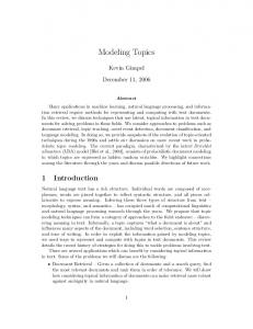
Figure 1. Approaches to semantic representation. (a) In a semantic network, words are represented as nodes, and edges indicate semantic relationships. (b) In a semantic space, words are represented as points, and proximity indicates semantic association. These are the first two dimensions of an LSA solution. The black dot is the origin. (c) In the topic model, words are represented as belonging to a set of probabilistic topics. The matrix shown on the left indicates the probability of each word under each of three topics. The three columns on the right show the words that appear in those topics, ordered from highest to lowest probability.

diction task is complicated by the fact that words have multiple senses: BANK should only influence the probabilities of FEDERAL and RESERVE if the gist of the sentence suggests the sense that refers to a financial institution. If words like STREAM or MEADOW also appear in the sentence, then it is likely that BANK refers to the side of a river, and words like WOODS or FIELD should increase in probability. Using the gist of sentences to predict and disambiguate words is an essential first step in linguistic processing (Ericsson & Kintsch, 1995; Kintsch, 1988; Potter, 1993). Our ability to extract gist has influences that reach beyond language processing, pervading even simple tasks such as memorizing lists of words. A number of studies have shown that when people try to remember a list of words that are all semantically associated with a word that does not appear on the list, the associated word intrudes upon their memory (Deese, 1959; McEvoy, Nelson, & Komatsu, 1999; Roediger, Watson, McDermott, & Gallo, 2001). Results of this kind have led to the development of dual-route memory models, which suggest that people encode not just the verbatim content of a list of words, but also their gist (Brainerd, Reyna, & Mojardin, 1999; Brainerd, Wright, & Reyna, 2002; Mandler, 1980). These models leave open the question of how the memory system identifies this gist. In this paper, we analyze the abstract computational problem of extracting and using the gist of a set of words, and examine how well different solutions to this problem correspond to human behavior. The key difference between these solutions is the way that they represent gist. Previous research has focused on two approaches to semantic representation: semantic networks (e.g., Collins & Loftus, 1975; Collins & Quillian, 1969) and semantic spaces (e.g., Landauer & Dumais, 1997; Lund & Burgess, 1996). Examples of these two representations are shown in Figure 1. We take a step back from these specific proposals, and provide a more general formulation of the computational problem that these representations are used to solve. We express the problem as one of statistical inference: given some data – the set of words – inferring the latent structure from which it was generated. Stating the problem in these terms makes it possible to explore forms of semantic representation that go beyond networks and spaces. Identifying the statistical problem underlying the extraction and use of gist makes it possible


3

to use any form of semantic representation: all that needs to be specified is a probabilistic process by which a set of words are generated using that representation of their gist. In machine learning and statistics, such a probabilistic process is called a generative model. Most computational approaches to natural language have tended to focus exclusively on either structured representations (e.g., Chomsky, 1965; Pinker, 1999) or statistical learning (e.g., Elman, 1990; Plunkett & Marchman, 1993). Generative models provide a way to combine the strengths of these two traditions, making it possible to use statistical methods to learn structured representations. As a consequence, generative models have recently become popular in both computational linguistics (e.g., Charniak, 1993; Jurafsky & Martin, 2000; Manning & Shütze, 1999) and psycholinguistics (e.g., Baldewein & Keller, 2004; Jurafsky, 1996), although this work has tended to emphasize syntactic structure over semantics. The combination of structured representations with statistical inference makes generative models the perfect tool for evaluating novel approaches to semantic representation. We use our formal framework to explore the idea that the gist of a set of words can be represented as a probability distribution over a set of topics. Each topic is a probability distribution over words, and the content of the topic is reflected in the words to which it assigns high probability. For example, high probabilities for WOODS and STREAM would suggest a topic refers to the countryside, while high probabilities for FEDERAL and RESERVE would suggest a topic refers to finance. A schematic illustration of this form of representation appears in Figure 1 (c). Following work in the information retrieval literature (Blei, Ng, & Jordan, 2003), we use a simple generative model that defines a probability distribution over a set of words, such as a list or a document, given a probability distribution over topics. Using methods developed in Bayesian statistics, a set of topics can be learned automatically from a collection of documents, as a computational analog of how human learners might discover semantic knowledge through their linguistic experience (Griffiths & Steyvers, 2002, 2003, 2004). The topic model provides a starting point for an investigation of new forms of semantic representation. Representing words using topics has an intuitive correspondence to feature-based models of similarity. Words that receive high probability under the same topics will tend to be highly predictive of one another, just as stimuli that share many features will be highly similar. We will show that this intuitive correspondence is supported by a formal correspondence between the topic model and Tversky’s (1977) feature-based approach to modeling similarity. Since the topic model uses exactly the same input as Latent Semantic Analysis (LSA; Landauer & Dumais, 1997), a leading model of the acquisition of semantic knowledge in which words are represented as points in a semantic space, we can compare these two models as a means of examining the implications of different kinds of semantic representation, just as featural and spatial representations have been compared as models of human similarity judgments (Tversky, 1977; Tversky & Gati, 1982; Tversky & Hutchinson, 1986). Furthermore, the topic model can easily be extended to capture other kinds of latent linguistic structure. Introducing new elements into a generative model is straightforward, and by adding components to the model that can capture richer semantic structure or rudimentary syntax we can begin to develop more powerful statistical models of language. The plan of the paper is as follows. First, we summarize previous approaches to semantic representation, considering their strengths and weaknesses. We then analyze the abstract computational problem of extracting and using gist, formulating this problem as one of statistical inference. The topic model is then introduced as one method for solving this computational problem. The body of the paper is concerned with assessing how well the representation recovered by the topic model


4

corresponds with human semantic memory. We compare our model with LSA in predicting three kinds of data: word association norms (Nelson, McEvoy, & Schreiber, 1998), free recall of word lists (Roediger, Watson, McDermott, & Gallo, 2001) and the senses of words (Miller & Fellbaum, 1998; Roget, 1911). In an analysis inspired by Tversky’s (1977) critique of spatial measures of similarity, we show that several aspects of word association that can be explained by the topic model are problematic for the spatial representation used by LSA. We also show that the topic model outperforms LSA in identifying the number of senses of a word and in predicting semantically-related intrusions in free recall. Finally, in the General Discussion, we consider some extensions of the topic model and discuss connections with previous research.

Approaches to semantic representation Psychological theories of semantic representation are typically based on one of two kinds of representation: semantic networks or semantic spaces. We will discuss these two approaches in turn, identifying some of their strengths and weaknesses. Semantic networks In a semantic network, such as that shown in Figure 1 (a), a set of words or concepts are represented as nodes connected by edges that indicate some kind of relationship. This relationship could be relatively complex, indicating properties or class membership and assuming an underlying inheritance hierarchy (Collins & Loftus, 1975; Collins & Quillian, 1969), or a simpler associative connection. Seeing a word activates its node, and activation spreads through the network, activating nodes that are nearby. The notion of spreading activation is relatively widespread in models of human memory, being used to explain a variety of phenomena related to semantic priming (Anderson, 1983; McNamara, 1992; McNamara & Altarriba, 1988). Semantic networks are an intuitive framework for expressing the semantic relationships between words. The profile of node activities provides an implicit representation of the gist of a set of words, and the notion of spreading activation gives a simple account of how this representation is used to predict which other words are likely to occur in a particular context. However, semantic networks face two significant problems as an account of human semantic representation. First, while it is clear how a semantic network could be used in prediction, it is not clear how that semantic network could itself be learned. A complete account of human semantic memory should not just explain how associations between words are used, but also account for why those associations are formed in the first place. Second, the notion of spreading activation has drawn criticism on both theoretical and empirical grounds (e.g., Markman, 1998). A basic problem is that it is not clear what activation means, or how the spread of activation through a network can be justified on a priori grounds. A more concrete concern is that there are experimental results that go against the simple idea of spreading activation. Spreading activation can explain why priming might have an excitatory effect on lexical decision. For example, a word like NURSE primes the word DOCTOR because it activates concepts that are closely related to DOCTOR, and the spread of activation ultimately activates doctor. However, not all priming effects are excitatory. For example, Neely (1976) showed that priming with irrelevant cues could have an inhibitory effect on lexical decision. To use an example from Markman (1998), priming with HOCKEY could produce a slower reaction time for DOCTOR than presenting a completely neutral prime. Inhibitory effects like these are difficult to explain in terms of spreading activation,


5

Document 10

20

30

40

50

60

70

80

90

BANK COMMERCIAL CRUDE DEEP DEPOSITS DRILL FEDERAL FIELD GASOLINE LOANS MEADOW MONEY OIL PETROLEUM RESERVE RIVER STREAM WOODS

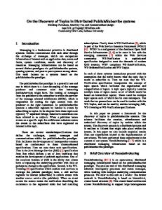
Figure 2. A word-document co-occurrence matrix, indicating the frequencies of 18 words across 90 documents extracted from the TASA corpus. Each row corresponds to a word in the vocabulary, and each column to a document in the corpus. Grayscale indicates the frequency of each word in each document, with black being the highest frequency and white being zero.

because there is no simple inhibitory relationship between just seem unrelated.

HOCKEY

and

DOCTOR :

the two words

Semantic spaces An alternative to semantic networks is the idea that the meaning of words can be captured using a spatial representation (Deese, 1959; Fillenbaum & Rapoport, 1971) In a semantic space, such as that shown in Figure 1 (b), words are nearby if they are similar in meaning. Several methods have recently been developed for extracting semantic spaces from text (Landauer & Dumais, 1997; Lund & Burgess, 1996). One such method, called Latent Semantic Analysis (LSA; Landauer & Dumais, 1997), is a procedure for extracting a spatial representation for words from a multi-document corpus of text. The input to LSA is a word-document co-occurrence matrix, such as that shown in Figure 2. In a word-document co-occurrence matrix, each row represents a word, each column represents a document, and the entries indicate the frequency with which that word occurred in that document. The matrix shown in Figure 2 is a portion of the full co-occurrence matrix for the TASA corpus, a collection of passages excerpted from educational texts used in curricula from the first year of school to the first year of college. This portion features 30 documents that use the word MONEY, 30 documents that use the word OIL, and 30 documents that use the word RIVER. The vocabulary is restricted to 18 words, and the entries indicate the frequency with which the 644 tokens of those words appeared in the 90 documents. The output from LSA is a spatial representation for words and documents. After applying various transformations to the entries in a word-document co-occurrence matrix (one standard set of transformations is described in Griffiths & Steyvers, 2003), singular value decomposition is used to factorize this matrix into three smaller matrices, U , D, and V , as shown in Figure 3 (a). Each of these matrices has a different intepretation. The U matrix provides an orthonormal basis for a space in which each word is a point. The D matrix, which is diagonal, is a set of weights for the dimensions of this space. The V matrix provides an orthonormal basis for a space in which each document is a point. An approximation to the original matrix of transformed counts can be obtained by remultiplying these matrices, but choosing to use only the initial portions of each matrix, corresponding to the use of a lower-dimensional spatial representation. In psychological applications of LSA, the critical result of this procedure is the first matrix, U , which provides a spatial representation for words. Figure 1 (b) shows the first two dimensions of U for the word-document co-occurence matrix shown in Figure 2. The results shown in the figure


probability distributions over words

topics

documents

P(w z)

P(z g)

topic distributions over words

topics

= words

words

P(w g)

D weights

V

T

document space

LSA

documents (b)

word space

dimensions

transformed word-document co-occurrence matrix

words

words

X

= U

documents

dimensions

dimensions

dimensions

documents (a)

6

document distributions over topics

Topic model

Figure 3. (a) Latent Semantic Analysis (LSA) performs dimensionality reduction using the singular value decomposition. The transformed word-document co-occurrence matrix, X, is factorized into three smaller matrices, U , D, and V . U provides an orthonormal basis for a spatial representation of words, D weights those dimensions, and V provides an orthonormal basis for a spatial representation of documents. (b) The topic model performs dimensionality reduction using statistical inference. The probability distribution over words for each document in the corpus conditioned upon its gist, P (w|g), is approximated by a weighted sum over a set of probabilistic topics, represented with probability distributions over words P (w|z), where the weights for each document are probability distributions over topics, P (z|g), determined by the gist of the document, g. As with LSA, this dimensionality reduction method can be written as a matrix factorization, although the constraints on the matrices involved and the cost function for the approximation are quite different: LSA finds a decomposition in terms of orthogonal matrices, minimizing squared error, while the topic model finds a decomposition in terms of stochastic matrices, with the maximum likelihood solution minimizing the Kullback-Leibler divergence (Cover & Thomas, 1991).

demonstrate that LSA identifies some appropriate clusters of words. For example, OIL, PETROLEUM and CRUDE are close together, as are FEDERAL, MONEY, and RESERVE. The word DEPOSITS lies between the two clusters, reflecting the fact that it can appear in either context. The cosine of the angle between the vectors corresponding to words in the semantic space defined by U has proven to be an effective measure of the semantic association between those words, as assessed on measures such as standardized tests of English fluency (Landauer & Dumais, 1997). The cosine of the angle between two vectors w1 and w2 (both rows of U , converted to column vectors) is w1T w2 cos(w1 , w2 ) = , (1) ||w1 ||||w2 || √ where w1T w2 is the inner product of the vectors w1 and w2 , and ||w|| denotes the norm, wT w. Performance in predicting human judgments is typically better when using only the first few hundred derived dimensions, since reducing the dimensionality of the representation can decrease the effects


7

of statistical noise and emphasize the latent correlations among words (Landauer & Dumais, 1997). Latent Semantic Analysis provides a simple procedure for extracting a spatial representation of the associations between words from a word-document co-occurrence matrix. The gist of a set of words is represented by the average of the vectors associated with those words. Applications of LSA often evaluate the similarity between two documents by computing the cosine between the average word vectors for those documents (Landauer & Dumais, 1997; Rehder, Schreiner, Wolfe, Laham, Landauer, & Kintsch, 1998; Wolfe, Schreiner, Rehder, Laham, Foltz, Kintsch, & Landauer, 1998). This representation of the gist of a set of words can be used to address the prediction problem: we should predict that words with vectors close to the gist vector are likely to occur in the same context. However, the representation of words as points in an undifferentiated Euclidean space makes it difficult for LSA to solve the disambiguation problem. The key issue is that this relatively unstructured representation does not explicitly identify the different senses of words. While DEPOSITS lies between words having to do with finance and words having to do with oil, the fact that this word has multiple senses is not encoded in the representation. Consequently, it is not clear how such a representation could be used to identify the sense in which a particular word is being used.

Extracting and using gist as statistical problems Semantic networks and semantic spaces are both proposals for a form of semantic representation that can be used to evaluate the similarity between words and make predictions about which words are likely to be observed in a particular context. We will now take a step back from these specific proposals, and consider the abstract computational problem that they are intended to solve, in the spirit of Marr’s (1982) notion of the computational level, and Anderson’s (1990) rational analysis. Our aim is to clarify the goals of the computation and to identify the logic by which these goals can be achieved, so that this logic can be used as the basis for exploring other approaches to semantic representation. Assume we have seen a sequence of words w = {w1 , w2 , . . . , wn }. These n words manifest some latent semantic structure ℓ. We will assume that ℓ consists of the gist of that sequence of words g, and the sense in which each word is being used, z = {z1 , z2 , . . . , zn }, so ℓ = (g, z). We can now identify three problems that the human memory system has to solve: Prediction Disambiguation Gist extraction

Predict wn+1 from w Infer z from w Infer g from w

Each of these problems can be formulated as statistical problems. The prediction problem requires computing the conditional probability of wn+1 given w, P (wn+1 |w). The disambiguation problem requires computing the conditional probability of z given w, P (z|w). The gist extraction problem requires computing the probability of g given w, P (g|w). All of the probabilities needed to solve the problems of prediction, disambiguation, and gist extraction can be computed from a single joint distribution over words and latent structures, P (w, ℓ). The problems of prediction, disambiguation, and gist extraction can thus be solved by learning the joint probabilities of words and latent structures. This can be done using a generative model for language. Generative models are widely used in machine learning and statistics as a means of learning structured probability distributions. A generative model specifies a hypothetical causal process by which data are generated, breaking this process down into probabilistic steps. Critically, this procedure can involve unobserved variables, corresponding to latent structure that


(a)

Latent structure

Words

w

ℓ

8

g

(b)

z1

z2

z3

z4

w1

w2

w3

w4

Figure 4. Generative models for language. (a) A schematic representation of generative models for language. Latent structure ℓ generates words w. This generative process defines a probability distribution over ℓ, P (ℓ), and w given ℓ, P (w|ℓ). Applying Bayes’ rule with these distributions makes it possible to invert the generative process, inferring ℓ from w. (b) Latent Dirichlet Allocation (Blei et al., 2003), a topic model. A document is generated by choosing a distribution over topics that reflects the gist of the document, g, choosing a topic zi for each potential word from a distribution determined by g, and then choosing the actual word wi from a distribution determined by zi .

plays a role in generating the observed data. Statistical inference can be used to identify the latent structure most likely to have been responsible for a set of observations. A schematic generative model for language is shown in Figure 4 (a). In this model, latent structure ℓ generates an observed sequence of words w = {w1 , . . . , wn }. This relationship is illustrated using graphical model notation (e.g., Jordan, 1998; Pearl, 1988). Graphical models provide an efficient and intuitive method of illustrating structured probability distributions. In a graphical model, a distribution is associated with a graph in which nodes are random variables and edges indicate dependence. Unlike artificial neural networks, in which a node typically indicates a single unidimensional variable, the variables associated with nodes can be arbitrarily complex. ℓ can be any kind of latent structure, and w represents a set of n words. The graphical model shown in Figure 4 (a) is a directed graphical model, with arrows indicating the direction of the relationship among the variables. The result is a directed graph, in which “parent” nodes have arrows to their “children”. In a generative model, the direction of these arrows specifies the direction of the causal process by which data are generated: a value is chosen for each variable by sampling from a distribution that conditions on the parents of that variable in the graph. The graphical model shown in the figure indicates that words are generated by first sampling a latent structure, ℓ, from a distribution over latent structures, P (ℓ), and then sampling a sequence of words, w, conditioned on that structure from a distribution P (w|ℓ). The process of choosing each variable from a distribution conditioned on its parents defines a joint distribution over observed data and latent structures. In the generative model shown in Figure 4 (a), this joint distribution is P (w, ℓ) = P (w|ℓ)P (ℓ). With an appropriate choice of ℓ, this joint distribution can be used to solve the problems of prediction, disambiguation, and gist extraction identified above. In particular, the probability of the latent


9

structure ℓ given the sequence of words w can be computed by applying Bayes’ rule: P (ℓ|w) =

P (w|ℓ)P (ℓ) P (w)

(2)

where P (w) =

X

P (w|ℓ)P (ℓ).

ℓ

This Bayesian inference involves computing a probability that goes against the direction of the arrows in the graphical model, inverting the generative process. Equation 2 provides the foundation for solving the problems of prediction, disambiguation, and gist extraction. If words are generated independently conditioned on ℓ, then P (wn+1 |w) can be written as X P (wn+1 |ℓ)P (ℓ|w), (3) P (wn+1 |w) = ℓ where P (wn+1 |ℓ) is specified by the generative process. Distributions over the senses of words, z, and their gist, g, can be computed by summing out the irrelevant aspect of ℓ, P (z|w) =

X

P (ℓ|w)

(4)

X

P (ℓ|w),

(5)

g

P (g|w) =

z

where we assume that the gist of a set of words takes on a discrete set of values – if it is continuous, then Equation 5 requires an integral rather than a sum. This abstract schema gives a general form common to all generative models for language. Specific models differ in the latent structure ℓ that they assume, the process by which this latent structure is generated (which defines P (ℓ)), and the process by which words are generated from this latent structure (which defines P (w|ℓ)). Most generative models that have been applied to language focus on latent syntactic structure (e.g., Charniak, 1993; Jurafsky & Martin, 2000; Manning & Shütze, 1999). In the next section, we will describe a generative model that represents the latent semantic structure that underlies a set of words.

Representing gist with topics A topic model is a generative model that assumes a latent structure ℓ = (g, z), representing the gist of a set of words, g, as a distribution over T topics, and the sense of the ith word, zi , as an assignment of that word to one of these topics. Each topic is a probability distribution over words. A document – a set of words – is generated by choosing the distribution over topics reflecting its gist, using this distribution to choose a topic zi for each word wi , and then generating the word itself from the distribution over words associated with that topic. Given the gist of the document in which it is contained, this generative process defines the probability of the ith word to be P (wi |g) =

T X

zi =1

P (wi |zi )P (zi |g),

(6)


10

in which the topics, specified by P (w|z), are mixed together with weights given by P (z|g), which vary across documents.1 The dependency structure among variables in this generative model is shown in Figure 4 (b). Intuitively, P (w|z) indicates which words are important to a topic, while P (z|g) is the prevalence of those topics in a document. For example, if we lived in a world where people only wrote about finance, the English countryside, and oil mining, then we could model all documents with the three topics shown in Figure 1 (c). The content of the three topics is reflected in P (w|z): the finance topic gives high probability to words like RESERVE and FEDERAL, the countryside topic gives high probability to words like STREAM and MEADOW, and the oil topic gives high probability to words like PETROLEUM and GASOLINE. The gist of a document, g, indicates whether a particular document concerns finance, the countryside, oil mining, or financing an oil refinery in Leicestershire, by termining the distribution over topics, P (z|g). Equation 6 gives the probability of a word conditioned on the gist of a document. We can define a generative model for a collection of documents by specifying how the gist of each document is chosen. Since the gist is a distribution over topics, this requires using a distribution over multinomial distributions. The idea of representing documents as mixtures of probabilistic topics has been used in a number of applications in information retrieval and statistical natural language processing, with different models making different assumptions about the origins of the distribution over topics (e.g., Bigi, De Mori, El Beze, & Spriet, 1997; Blei et al., 2003; Hofmann, 1999; Iyer & Ostendorf, 1996; Ueda & Saito, 2003). We will use a generative model introduced by Blei et al. (2003) called Latent Dirichlet Allocation. In this model, the multinomial distribution representing the gist is drawn from a from a Dirichlet distribution, a standard probability distribution over multinomials. Having defined a generative model for a corpus based upon some parameters, it is possible to use statistical methods to infer the parameters from the corpus. In our case, this means finding a set of topics such that each document can be expressed as a mixture of those topics. An algorithm for extracting a set of topics is described in the Appendix, and a more detailed description and application of this algorithm can be found in Griffiths and Steyvers (2004). This algorithm takes as input a word-document co-occurrence matrix. The output is a set of topics, each being a probability distribution over words. The topics shown in Figure 1 (c) are actually the output of this algorithm when applied to the word-document co-occurrence matrix shown in Figure 2. These results illustrate how well the topic model handles words with multiple senses: FIELD appears in both the oil and countryside topics, BANK appears in both finance and countryside, and DEPOSITS appears in both oil and finance. The different topics thus capture different senses of these words. This is a key advantage of the topic model: by assuming a more structured representation, in which words are assumed to belong to topics, different senses of words can be differentiated. Prediction, disambiguation, and gist extraction The topic model provides a direct solution to the problems of prediction, disambiguation, and gist extraction identified in the previous section. The details of these computations are presented in the Appendix. To illustrate how these problems are solved by the model, we will consider a simplified case where all words in a sentence are assumed to have the same topic. In this case g is 1 We have suppressed the dependence of the probabilities discussed in this section on the parameters specifying P (w|z) and P (z|g), assuming that these parameters are known. A more rigorous treatment of the computation of these probabilities is given in the Appendix.


11

a distribution that puts all of its probability on a single topic, z, and zi = z for all i. This “single topic” assumption makes the mathematics straightforward, and is a reasonable assumption about the nature of communicative discourse.2 Under the single topic assumption, disambiguation and gist extraction become equivalent: the senses and the gist of a set of words are both expressed in the single topic, z, that was responsible for generating words w = {w1 , w2 , . . . , wn }. Applying Bayes’ rule, we have P (z|w) = =

P (w|z)P (z) P (w) Qn i=1 P (wi |z)P (z) P Q , n z i=1 P (wi |z)P (z)

(7)

where we have used the fact that the wi are independent given z. If we assume a uniform prior over topics, P (z) = T1 , the distribution over topics depends only on the product of the probabilities of each of the wi under each topic z. The product acts like a logical “and”: a topic will only be likely if it gives reasonably high probability to all of the words. Figure 5 shows how this functions to disambiguate words, using the topics from Figure 1. On seeing the word BANK, both the finance and the countryside topics have high probability. Seeing STREAM quickly swings the probability in favor of the bucolic interpretation. Solving the disambiguation problem is the first step in solving the prediction problem. Following Equation 3, we have P (wn+1 |w) =

X z

P (wn+1 |z)P (z|w).

(8)

The predicted distribution over words is thus a mixture of topics, with each topic being weighted by the distribution computed in Equation 7. This is illustrated in Figure 5: on seeing BANK, the predicted distribution over words is a mixture of the finance and countryside topics, but STREAM moves this distribution towards the countryside topic. Topics and semantic networks The topic model provides a clear way of thinking about how and why “activation” might spread through a semantic network, and can also explain inhibitory priming effects. The standard conception of a semantic network is a graph with edges between word nodes, as shown in Figure 6 (a). Such a graph is unipartite: there is only one type of node, and those nodes can be interconnected freely. In contrast, bipartite graphs consist of nodes of two types, and only nodes of different types can be connected. We can form a bipartite semantic network by introducing a second class of nodes that mediate the connections between words. One way to think about the representation of the meanings of words provided by the topic model is in terms of the bipartite semantic network shown in Figure 6 (b), where the second class of nodes are the topics. 2 It is also possible to define a generative model that makes this assumption directly, having just one topic per sentence, and to use techniques like those described in the Appendix to identify topics using this model. We did not use this model because it uses additional information about the structure of the documents, making it harder to compare against alternative approaches like Latent Semantic Analysis (Landauer & Dumais, 1997). The single topic assumption can also be derived as the consequence of having a hyperparameter α favoring choices of z that employ few topics: the single topic assumption is produced by allowing α to approach 0.


BANK STREAM

Probability

BANK

1

1

0.5

0.5

0

1

2 Topic

12

0

3


1

2 Topic

3


0

0.2 Probability

0.4

0

0.2 Probability

0.4

Figure 5. Prediction and disambiguation. (a) Words observed in a sentence, w. (b) The distribution over topics conditioned on those words, P (z|w). (c) The predicted distribution over words resulting from sumP ming over this distribution over topics, P (wn+1 |w) = z P (wn+1 |z)P (z|w). On seeing BANK, the model is unsure whether the sentence concerns finance or the countryside. Subsequently seeing STREAM results in a strong conviction that BANK does not refer to a financial institution.

(a)

(b)

word

topic

topic

word word word

word

word

word

word

Figure 6. Semantic networks. (a) In a unipartite network, there is only one class of nodes. In this case, all nodes represent words. (b) In a bipartite network, there are two classes, and connections only exist between nodes of different classes. In this case, one class of nodes represents words and the other class represents topics.


13

In any context, there is uncertainty about which topics are relevant to that context. On seeing a word, the probability distribution over topics moves to favor the topics associated with that word: P (z|w) moves away from uniformity. This increase in the probability of those topics is intuitively similar to the idea that activation spreads from the words to the topics that are connected with them. Following Equation 8, the words associated with those topics also receive higher probability. This dispersion of probability throughout the network is again reminiscent of spreading activation. However, there is an important difference between spreading activation and probabilistic inference: the probability distribution over topics, P (z|w) is constrained to sum to one. This means that as the probability of one topic increases, the probability of another topic decreases. The constraint that the probability distribution over topics sums to one is sufficient to allow the phenomenon of inhibitory priming discussed above. Inhibitory priming occurs as a necessary consequence of excitatory priming: when the probability of one topic increases, the probability of another topic decreases. Consequently, it is possible for one word to decrease the predicted probability with which another word will occur in a particular context. For example, according to the topic model, the probability of the word DOCTOR is 0.000334. Under the single topic assumption, the probability of the word DOCTOR conditioned on the word NURSE is 0.0071, an instance of excitatory priming. However, the probability of DOCTOR drops to 0.000081 when conditioned on HOCKEY . The word HOCKEY suggests that the topic concerns sports, and consequently topics that give DOCTOR high probability have lower weight in making predictions. By incorporating the constraint that probabilities sum to one, generative models are able to capture both the excitatory and the inhibitory influence of information. Topics and Latent Semantic Analysis Latent Semantic Analysis has a number of similarities with the topic model introduced above. Indeed, the probabilistic topic model developed by Hofmann (1999) was motivated by the success of LSA, and provided the inspiration for the model introduced by Blei et al. (2003) that we use here. Both LSA and the topic model take a word-document co-occurrence matrix as input. Both LSA and the topic model provide a representation of the gist of a document, either as a point in space or a distribution over topics. And both LSA and the topic model can be viewed as a form of “dimensionality reduction”, attempting to find a lower-dimensional representation of the structure expressed in a collection of documents. In the topic model, this dimensionality reduction consists of trying to express the large number of probability distributions over words provided by the different documents in terms of a small number of topics, as illustrated in Figure 3 (b). However, there are two important differences between LSA and the topic model. The major difference, to which we will return in the General Discussion, is that LSA is not a generative model. It does not identify the causal process responsible for generating documents, and the role of the meanings of words in this process. As a consequence, it is difficult to extend LSA to incorporate different kinds of semantic structure, or to recognize the syntactic roles that words play in a document. This leads to the second difference between LSA and the topic model: the nature of the representation. Latent Semantic Analysis is based upon the singular value decomposition, a method from linear algebra that can only yield a representation of the meanings of words as points in an undifferentiated Euclidean space. In contrast, the statistical inference techniques used with generative models are flexible, and make it possible to use structured representations. The topic model provides a simple structured representation: a set of individually meaningful topics, and information about which words belong to those topics. We will show that even this simple structure is sufficient


14

to allow the topic model to capture some of the qualitative features of word association that prove problematic for LSA, and to predict quantities that cannot be predicted by LSA, such as the number of senses of a word.

Comparing topics and spaces The topic model provides a solution to extracting and using the gist of set of words. In this section, we will evaluate the topic model as a psychological account of the content of human semantic memory, comparing its performance with LSA. The topic model and LSA both use the same input – a word-document co-occurrence matrix – but they differ in how this input is analyzed, and in the way that they represent the gist of documents and the meaning of words. By comparing these models, we hope to demonstrate the utility of generative models for exploring questions of semantic representation, and to gain some insight into the strengths and limitations of different kinds of representation. Our comparison of the topic model and LSA will have three components. First, we will evaluate the predictions of the two models using a word association task, considering both the quantitative and the qualitative properties of these predictions. In particular, we will show that the topic model can explain several phenomena of word association that are problematic for Latent Semantic Analysis. These phenomena are analogues of the phenomena of similarity judgments that are problematic for spatial models of similarity (Tversky, 1977; Tversky & Gati, 1982; Tversky & Hutchinson, 1986). Second, we will demonstrate that the topic model also outperforms LSA in a setting that requires integrating semantic information across multiple words: predicting semantic intrusions in free recall. Finally, we will show that the simple structured representation assumed by the topic model makes it possible to predict quantities that cannot be predicted by LSA, such as the number of senses of a word. Quantitative predictions for word association Are there any more fascinating data in psychology than tables of association? Deese (1965, p. viii) Association has been part of the theoretical armory of cognitive psychologists since Thomas Hobbes used the notion to account for the structure of our “Trayne of Thoughts” (Hobbes, 1651/1998; detailed histories of association are provided by Deese, 1965, and Anderson & Bower, 1974). One of the first experimental studies of association was conducted by Galton (1880), who used a word association task to study different kinds of association. Since Galton, several psychologists have tried to classify kinds of association or to otherwise divine its structure (e.g., Deese, 1962; 1965). This theoretical work has been supplemented by the development of extensive word association norms, listing commonly named associates for a variety of words (e.g., Cramer, 1968; Kiss, Armstrong, Milroy, & Piper, 1973; Nelson, McEvoy & Schreiber, 1998). These norms provide a rich body of data, which has only recently begun to be addressed using computational models (Dennis, 2003; Nelson, McEvoy, & Dennis, 2000). While, unlike Deese (1965), we suspect that there may be more fascinating psychological data than tables of associations, word association provides a useful benchmark for evaluating models of human semantic representation. The relationship between word association and semantic representation is analogous to that between similarity judgments and conceptual representation,


15

being an accessible behavior that provides clues and constraints that guide the construction of psychological models. Also, like similarity judgments, association scores are highly predictive of other aspects of human behavior. Word association norms are commonly used in constructing memory experiments, and statistics derived from these norms have been shown to be important in predicting cued recall (Nelson, McKinney, Gee, & Janczura, 1998), recognition (Nelson, McKinney, et al., 1998; Nelson, Zhang, & McKinney, 2001), and false memories (Deese, 1959; McEvoy, Nelson, & Komatsu, 1999; Roediger, Watson, McDermott, & Gallo, 2001). It is not our goal to develop a model of word association, as many factors other than semantic association are involved in this task (e.g., Ervin, 1961; McNeill, 1966), but we believe that issues raised by word association data can provide insight into models of semantic representation. We used the norms of Nelson et al. (1998) to evaluate the performance of LSA and the topic model in predicting human word association. These norms were collected using a free association task, in which participants were asked to produce the first word that came into their head in response to a cue word. The results are unusually complete, with associates being derived for every word that was produced more than once as an associate for any other word. For each word, the norms provide a set of associates and the frequencies with which they were named, making it possible to compute the probability distribution over associates for each cue. We will denote this distribution P (w2 |w1 ) for a cue w1 and associate w2 , and order associates by this probability: the first associate has highest probability, the second next highest, and so forth. We obtained predictions from the two models by deriving semantic representations from the TASA corpus, which is a collection of excerpts from reading materials commonly encountered between the first year of school and the first year of college. We used a smaller vocabulary than previous applications of LSA to TASA, considering only words that occurred at least 10 times in the corpus and were not included in a standard “stop” list containing function words and other high frequency words with low semantic content. This left us with a vocabulary of 26,243 words, of which 4,235,314 tokens appeared in the 37,651 documents contained in the corpus. We used the singular value decomposition to extract a 700 dimensional representation of the word-document cooccurrence statistics, and examined the performance of the cosine as a predictor of word association using this and a variety of subspaces of lower dimensionality. Our choice to use 700 dimensions as an upper limit was guided by two factors, one theoretical and the other practical: previous analyses suggested that the performance of LSA was best with only a few hundred dimensions (Landauer & Dumais, 1997), an observation that was consistent with performance on our task, and 700 dimensions is the limit of most algorithms for singular value decomposition with a matrix of this size on a workstation with 2GB of RAM. We applied the algorithm for finding topics described in the Appendix to the same worddocument co-occurrence matrix, extracting representations with up to 1700 topics. Our algorithm is far more memory efficient than the singular value decomposition, as all of the information required throughout the computation can be stored in sparse matrices. Consequently, we ran the algorithm at increasingly high dimensionalities, until prediction performance began to level out. In each case, the set of topics found by the algorithm was highly interpretable, expressing different aspects of the content of the corpus. A selection of topics from the 1700 topic solution are shown in Figure 7. The topics found by the algorithm are extremely intepretable, and pick out some of the key notions addressed by documents in the corpus, including very specific subjects like printing and combustion engines. The topics are extracted purely on the basis of the statistical properties of the words involved – roughly, that these words seem to appear in the same documents – and the

TOPICS IN SEMANTIC ASSOCIATION PRINTING PAPER PRINT PRINTED TYPE PROCESS INK PRESS IMAGE PRINTER PRINTS PRINTERS COPY COPIES FORM OFFSET GRAPHIC SURFACE PRODUCED CHARACTERS

PLAY PLAYS STAGE AUDIENCE THEATER ACTORS DRAMA SHAKESPEARE ACTOR THEATRE PLAYWRIGHT PERFORMANCE DRAMATIC COSTUMES COMEDY TRAGEDY CHARACTERS SCENES OPERA PERFORMED

TEAM GAME BASKETBALL PLAYERS PLAYER PLAY PLAYING SOCCER PLAYED BALL TEAMS BASKET FOOTBALL SCORE COURT GAMES TRY COACH GYM SHOT

JUDGE TRIAL COURT CASE JURY ACCUSED GUILTY DEFENDANT JUSTICE EVIDENCE WITNESSES CRIME LAWYER WITNESS ATTORNEY HEARING INNOCENT DEFENSE CHARGE CRIMINAL

HYPOTHESIS EXPERIMENT SCIENTIFIC OBSERVATIONS SCIENTISTS EXPERIMENTS SCIENTIST EXPERIMENTAL TEST METHOD HYPOTHESES TESTED EVIDENCE BASED OBSERVATION SCIENCE FACTS DATA RESULTS EXPLANATION

STUDY TEST STUDYING HOMEWORK NEED CLASS MATH TRY TEACHER WRITE PLAN ARITHMETIC ASSIGNMENT PLACE STUDIED CAREFULLY DECIDE IMPORTANT NOTEBOOK REVIEW

16 CLASS MARX ECONOMIC CAPITALISM CAPITALIST SOCIALIST SOCIETY SYSTEM POWER RULING SOCIALISM HISTORY POLITICAL SOCIAL STRUGGLE REVOLUTION WORKING PRODUCTION CLASSES BOURGEOIS

ENGINE FUEL ENGINES STEAM GASOLINE AIR POWER COMBUSTION DIESEL EXHAUST MIXTURE GASES CARBURETOR GAS COMPRESSION JET BURNING AUTOMOBILE STROKE INTERNAL

Figure 7. A sample of 1700 topics derived from the TASA corpus. Each column contains the 20 highest probability words in a single topic, as indicated by P (w|z). Words in boldface occur in different senses in neighboring topics, illustrating how the model deals with polysemy and homonymy. These topics were discovered in a completely unsupervised fashion, using just word-document co-occurrence frequencies.

algorithm does not require any special initialization or other human guidance. The topics shown in the figure were chosen to be representative of the output of the algorithm, and to illustrate how polysemous and homonymous words are represented in the model: different topics capture different contexts in which words are used, and thus different senses. For example, the first two topics shown in the figure capture two different senses of CHARACTERS: the symbols used in printing, and the personas in a play. To model word association with the topic model, we need to specify a probabilistic quantity that corresponds to the strength of association. The discussion of the problem of prediction above suggests a natural measure of semantic association: P (w2 |w1 ), the probability of word w2 given word w1 . Using the single topic assumption, we have P (w2 |w1 ) =

X z

P (w2 |z)P (z|w1 ),

(9)

which is just Equation 8 with n = 1. The details of evaluating this probability are given in the Appendix. This conditional probability automatically compromises between word frequency and semantic relatedness: higher frequency words will tend to have higher probabilities across all topics, and this will be reflected in P (w2 |z), but the distribution over topics obtained by conditioning on w1 , P (z|w1 ), will ensure that semantically related topics dominate the sum. If w1 is highly diagnostic of a particular topic, then that topic will determine the probability distribution over w2 . If w1 provides no information about the topic, then P (w2 |w1 ) will be driven by word frequency. The overlap between the words used in the norms and the vocabulary derived from TASA was 4,471 words, and all analyses presented in this paper are based on the subset of the norms that uses these words. Our evaluation of the two models in predicting word association was based upon two performance measures: the median rank of the first five associates under the ordering imposed by the cosine or the conditional probability, and the probability of the first associate being included in sets of words derived from this ordering. For LSA, the first of these measures was assessed by computing the cosine for each word w2 with each cue w1 , ranking the choices of w2 by cos(w1 , w2 ) such that the highest ranked word had highest cosine, and then finding the ranks of the first five associates for that cue. After applying this procedure to all 4, 471 cues, we computed the median ranks for each of the first five associates. An analogous procedure was performed with


17

the topic model, using P (w2 |w1 ) in the place of cos(w1 , w2 ). The second of our measures was the probability that the first associate is included in the set of the m words with the highest ranks under each model, varying m. These two measures are complementary: the first indicates central tendency, while the second gives the distribution of the rank of the first associate. The topic model outperforms LSA in predicting associations between words. The results of our analyses are shown in Figure 8. We tested LSA solutions with 100, 200, 300, 400, 500, 600 and 700 dimensions. In predicting the first associate, performance levels out at around 500 dimensions, being approximately the same at 600 and 700 dimensions. We will use the 700 dimensional solution for the remainder of our analyses, although our points about the qualitative properties of LSA hold regardless of dimensionality. The median rank of the first associate in the 700 dimensional solution was 31 out of 4470, and the word with highest cosine was the first associate in 11.54% of cases. We tested the topic model with 500, 700, 900, 1100, 1300, 1500, and 1700 topics, finding that performance levels out at around 1500 topics. We will use the 1700 dimensional solution for the remainder of our analyses. The median rank of the first associate in P (w2 |w1 ) was 18, and the word with highest probability under the model was the first associate in 16.15% of cases, in both cases an improvement of around 40 percent on LSA. The performance of both models on the two measures was far better than chance, which would be 2235.5 and 0.02% for the median rank and the proportion correct respectively. The dimensionality reduction performed by the models seems to improve predictions. The conditional probability P (w2 |w1 ) computed directly from the frequencies with which words appeared in different documents gave a median rank of 50.5 and predicted the first associate correctly in 10.24% of cases. Latent Semantic Analysis thus improved on the raw co-occurrence probability by between 20 and 40 percent, while the topic model gave an improvement of over 60 percent. In both cases, this improvement results purely from having derived a lower-dimensional representation from the raw frequencies. Figure 9 shows some examples of the associates produced by people and by the two different models. The figure shows two examples randomly chosen from each of four sets of cues: those for which both models correctly predict the first associate, those for which only the topic model predicts the first associate, those for which only LSA predicts the first associate, and those for which neither model predicts the first associate. These examples help to illustrate how the two models sometimes fail. For example, LSA sometimes latches onto the wrong sense of a word, as with PEN, and tends to give high scores to inappropriate low-frequency words like WHALE, COMMA, and MILDEW. Both models sometimes pick out correlations between words that do not occur for reasons having to do with the meaning of those words: BUCK and BUMBLE both occur with DESTRUCTION in a single document, which is sufficient for these low frequency words to become associated. In some cases, as with RICE, the most salient properties of an object are not those that are reflected in its use, and the models fail despite producing meaningful, semantically-related predictions. Qualitative properties of word association Quantitative measures like those shown in Figure 8 provide a simple means of summarizing the performance of the two models. However, they mask some of the deeper qualitative differences that result from using different kinds of representations. In his 1977 paper Features of similarity (and subsequently, Tversky & Gati, 1982; Tversky & Hutchinson, 1986), Amos Tversky famously argued against spatial representations of the similarity between conceptual stimuli. Tversky’s argument was founded upon violations of the metric axioms in similarity judgments. Specifically, similarity


18

First associate 100 Median rank

(a)

(b) 50

0

0.6

Median rank

Second associate 160 100 0.5 P(set contains first associate)

40

Median rank

Third associate 200 140 80

Median rank

Fourth associate 240

0.4

0.3

170 100

Median rank

Fifth associate 280 200 120

Cosine

Inner

Topics

Frequency 0.2 700/1700 600/1500 500/1300 400/1100 300/900 0.1 0 10 200/700 100/500

Frequency Best cosine Best inner 1700 topics 1

10 Set size

2

10

Figure 8. Performance of LSA and the topic model in predicting word association. (a) The median ranks of the first five associates under different measures of semantic association and different dimensionalities. Smaller ranks indicate better performance. The dotted line shows baseline performance, corresponding to the use of the raw frequencies with which words occur in the same documents. (b) The probability that a set containing the m highest ranked words under the different measures would contain the first association, with plot markers corresponding to m = 1, 5, 10, 25, 50, 100. The dotted line is baseline performance derived from co-occurrence frequency.

can be asymmetric, since the similarity of x to y can differ from the similarity of y to x, violates the triangle inequality, since x can be similar to y and y to z without x being similar to z, and shows a neighborhood structure inconsistent with the constraints imposed by spatial representations. Tversky concluded that conceptual stimuli are better represented in terms of sets of features. Tversky’s arguments about the adequacy of spaces and features for capturing the similarity between conceptual stimuli have direct relevance to the investigation of semantic representation. Words are conceptual stimuli, and Latent Semantic Analysis assumes that words can be represented as points in a space. The cosine, the standard measure of association used in LSA, is a monotonic function of the angle between two vectors in a high dimensional space. The angle between two vectors is a metric, satisfying the metric axioms of being zero for identical vectors, being symmetric, and obeying the triangle inequality. Consequently, the cosine exhibits many of the constraints of a metric. The topic model does not suffer from the same constraints. In fact, the topic model can be thought of as providing a feature-based representation for the meaning of words, with the topics under which a word has high probability being its features. In the Appendix, we show that there is actually a formal correspondence between evaluating P (w2 |w1 ) using Equation 9 and computing


CURB

Both

Topics only

LSA only

Neither

Cue

Cue

Cue

Cue

UNCOMMON Associates

STREET SIDEWALK ROAD CAR TIRE

PEN

COMMON RARE WEIRD UNUSUAL UNIQUE

PENCIL INK PAPER WRITE

COMMON FREQUENT CIRCUMSTANCE COUPLE WHALE (1)

HOG HEN NAP FIX MOP (7)

Topics STREET CAR CORNER WALK SIDEWALK (1)

SKILLET

Associates

LSA STREET PEDESTRIAN TRAFFIC SIDEWALK AVENUE (1)

19

COMMON CASE BIT EASY KNOWLEDGE (1)

DESTRUCTION

PAN FRY EGG COOK IRON

DESTROY WAR RUIN DEATH KILL

COOKING COOKED OVEN FRIED COOK (6)

DESTROY VULNERABLE BUMBLE THREAT BOMB (1)

LSA

PAN KITCHEN COOKING STOVE POT (1)

RICE

Associates DOG DIRTY DIRT STRIPES DARK

DIVIDE INDEPENDENT MIXTURE ACCOUNT COMMA (1)

SPOT GIRAFFE GRAY HIKE MILDEW (2972)

CHINESE WEDDING FOOD WHITE CHINA LSA

Topics WAR BUCK TAP NUCLEAR DAMAGE (24)

SPOTS

DIVIDE DIVORCE PART SPLIT REMOVE LSA

Topics PENCIL FOUNTAIN INK PAPER WRITE (1)

SEPARATE

Associates

PADDY HARVEST WHEAT BARLEY BEANS (322)

Topics FORM SINGLE DIVISION COMMON DIVIDE (5)

SPOT FOUND GIRAFFE BALD COVERED (1563)

VILLAGE CORN WHEAT GRAIN FOOD (68)

Figure 9. Actual and predicted associates for a subset of cues. Two cues were randomly selected from the sets of cues for which (from left to right) both models correctly predicted the first associate, only the topic model made the correct prediction, only LSA made the correct prediction, and neither model made the correct prediction. Each column lists the cue, human associates, predictions of the topic model, and predictions of LSA, presenting the first five words in order. The rank of the first associate is given in parentheses below the predictions of the topic model and LSA.

similarity in one of Tversky’s (1977) feature-based models. The association between two words is increased by each topic that assigns high probability to both, and decreased by topics that assign high probability to one but not the other, in the same way that common and distinctive features affect similarity. The two models we have been considering thus correspond to the two kinds of representation considered by Tversky. Word association also exhibits phenomena that parallel Tversky’s analyses of similarity, being inconsistent with the metric axioms. We will discuss three qualitative phenomena of word association – effects of word frequency, violation of the triangle inequality, and the large scale structure of semantic networks – connecting these phenomena to the notions used in Tversky’s (1977; Tversky & Gati, 1982; Tversky & Hutchinson, 1986) critique of spatial representations. We will show that LSA cannot explain these phenomena, due to the constraints that arise from the use of a spatial representation, but that these phenomena emerge naturally when words are represented using topics, just as they can be produced using feature-based representations for similarity. Tversky’s argument was not against spatial representations per se, but against the idea that similarity is a monotonic function of a metric, such as distance in psychological space (c.f. Shepard, 1987). Each of the phenomena he noted – asymmetry, violation of the triangle inequality, and neighborhood structure – could be produced from a spatial representation under a sufficiently creative scheme for assessing similarity. Asymmetry provides an excellent example, as several methods for producing asymmetries from spatial representations have already been suggested (Krumhansl, 1978; Nosofsky, 1991). However, his argument shows that the distance between two points in psychological space should not be taken as an absolute measure of the similarity between the objects that correspond to those points. Analogously, our results suggest that the cosine should not be taken as an absolute measure of the association between two words. They also reveal some surprising


20

properties of LSA, such as poor performance with words that have multiple senses, and suggest some reasons behind this poor performance. Asymmetries and word frequency. The asymmetry of similarity judgments was one of Tversky’s (1977) objections to the use of spatial representations for similarity. By definition, any metric d has to be symmetric: d(x, y) = d(y, x). If similarity is a function of distance, similarity should also be symmetric. However, it is possible to find stimuli for which people produce asymmetric similarity judgments. One classic example involves China and North Korea: people typically have the intuition that North Korea is more similar to China than China is to North Korea. Tversky’s explanation for this phenomenon appealed to the distribution of features across these objects: our representation of China involves a large number of features, only some of which are shared with North Korea, while our representation of North Korea involves a small number of features, many of which are shared with China. Word frequency is an important determinant of whether a word will be named as an associate. This can be seen by looking for asymmetric associations: pairs of words w1 , w2 in which one word is named as an associate of the other much more often than vice versa (i.e. either P (w2 |w1 ) >> P (w1 |w2 ) or P (w1 |w2 ) >> P (w2 |w1 )). The effect of word frequency can then be evaluated by examining the extent to which the observed asymmetries can be accounted for by the frequencies of the words involved. We defined two words w1 , w2 to be associated if one word was named as an associate of the other at least once (i.e. either P (w2 |w1 ) or P (w1 |w2 ) > 0), and assessed asymmetries in association by computing the ratio of cue-associate probabilities for all (w2 |w1 ) associated words, PP (w . Of the 45,063 pairs of associated words in our subset of the norms, 1 |w2 ) 38,744 (85.98%) had ratios indicating a difference in probability of at least an order of magnitude as a function of direction of association. Good examples of asymmetric pairs include KEG - BEER, TEXT- BOOK , TROUSERS - PANTS , MEOW- CAT and COBRA - SNAKE . In each of these cases, the first word elicits the second as an associate with high probability, while the second is unlikely to elicit the first. Of the 38,744 asymmetric associations, 30,743 (79.35%) could be accounted for by the frequencies of the words involved, with the higher frequency word being named as an associate more often. Latent Semantic Analysis does not predict word frequency effects, including asymmetries in association. The cosine is used as a measure of the semantic similarity between two words partly because it counteracts the effect of word frequency. The cosine is also inherently symmetric, as can be seen from Equation 1: cos(w1 , w2 ) = cos(w2 , w1 ) for all words w1 , w2 . This symmetry means that the model cannot predict asymmetries in word association without adopting a more complex measure of the similarity between words (c.f. Krumhansl, 1978; Nosofsky, 1991). In contrast, the topic model can predict the effect of frequency on word association. Word frequency is one of the factors that contributes to P (w2 |w1 ). The model can account for the asymmetries in the word association norms. As a conditional probability, P (w2 |w1 ) is inherently asymmetric, and the model correctly predicted the direction of 30, 905 (79.77%) of the 38, 744 asymmetric associations, including all of the examples given above. The topic model thus accounted for almost exactly the same proportion of asymmetries as word frequency – the difference was not statistically significant (χ2 (1) = 2.08, p = 0.149). The explanation for asymmetries in word association provided by the topic model is extremely similar to Tversky’s (1977) explanation for asymmetries in similarity judgments. Following Equation 9, P (w2 |w1 ) reflects the extent to which the topics in which w1 appears give high proba-


21

bility to topic w2 . High frequency words tend to appear in more topics than low frequency words. If wh is a high frequency word and wl is a low frequency word, wh is likely to appear in many of the topics in which wl appears, but wl will appear in only a few of the topics in which wh appears. Consequently, P (wh |wl ) will be large, but P (wl |wh ) will be small. Violation of the triangle inequality. The triangle inequality is another of the metric axioms: for a metric d, d(x, z) ≤ d(x, y) + d(y, z). This is referred to as the triangle inequality because if x, y, and z are interpreted as points comprising a triangle, it indicates that no side of that triangle can be longer than the sum of the other two sides. This inequality places strong constraints on distance measures, and strong constraints on the locations of points in a space given a set of distances. If similarity is assumed to be a monotonically decreasing function of distance, then this inequality translates into a constraint on similarity relations: if x is similar to y and y is similar to z, then x must be similar to z. Tversky and Gati (1982) provided several examples where this relationship does not hold. These examples typically involve shifting the features on which similarity is assessed. For instance, taking an example from William James (1890), a gas jet is similar to the moon, since both cast light, and the moon is similar to a ball, because of its shape, but a gas jet is not at all similar to a ball. Word association violates the triangle inequality. A triangle inequality in association would mean that if P (w2 |w1 ) is high, and P (w3 |w2 ) is high, then P (w3 |w1 ) must be high. It is easy to find sets of words that are inconsistent with this constraint. For example ASTEROID is highly associated with BELT, and BELT is highly associated with BUCKLE, but ASTEROID and BUCKLE have little association. Such cases are the rule rather than the exception, as shown in Figure 10 (a). Each of the histograms shown in the figure was produced by selecting all sets of three words w1 , w2 , w3 such that P (w2 |w1 ) and P (w3 |w2 ) were greater than some threshold τ , and computing the distribution of P (w3 |w1 ). Regardless of the value of τ , there exist a great many triples in which w1 and w3 are so weakly associated as not to be named in the norms. Latent Semantic Analysis cannot explain violations of the triangle inequality. As a monotonic function of the angle between two vectors, the cosine obeys an analogue of the triangle inequality. Given three vectors w1 , w2 , and w3 , the angle between w1 and w3 must be less than or equal to the sum of the angle between w1 and w2 and the angle between w2 and w3 . Consequently, cos(w1 , w3 ) must be greater than the cosine of the sum of the w1 − w2 and w2 − w3 angles. Using the trigonometric expression for the cosine of the sum of two angles, we obtain the inequality cos(w1 , w3 ) ≥ cos(w1 , w2 ) cos(w2 , w3 ) − sin(w1 , w2 ) sin(w2 , w3 ), where sin(w1 , w2 ) can be defined analogously to Equation 1. This inequality restricts the possible relationships between three words: if w1 and w2 are highly associated, and w2 and w3 are highly associated, then w1 and w3 must be highly associated. Figure 10 (b) shows how the triangle inequality manifests in LSA. High values of cos(w1 , w2 ) and cos(w2 , w3 ) induce high values of cos(w1 , w3 ). The implications of the triangle inequality are made explicit in Figure 10 (d): even for the lowest choice of threshold, the minimum value of cos(w1 , w3 ) was above the 97th percentile of cosines between all words in the corpus. The expression of the triangle inequality in LSA is subtle. It is hard to find triples for which a high value of cos(w1 , w2 ) and cos(w2 , w3 ) induce a high value of cos(w1 , w3 ), although ASTEROID BELT- BUCKLE is one such example: of the 4470 words in the norms (excluding self associations), BELT has the 13th highest cosine with ASTEROID , BUCKLE has the second highest cosine with BELT ,

TOPICS IN SEMANTIC ASSOCIATION Association

LSA

τ=0

(a)

(b)

22

Topics

τ = −1

τ=0

(c)

(d)

100

τ = 0.2

τ = 0.7

τ = 0.04

τ = 0.25

τ = 0.05

τ = 0.35

τ = 0.8

τ = 0.06

τ = 0.45

τ = 0.85

τ = 0.08

τ = 0.55

0

0.5 P( w | w ) 3

τ = 0.75

1

τ = 0.9

1

3

1

0

0.5 P( w | w ) 3

1

70 60 50 40 30 20

LSA Lower bound from triangle inequality Topics

10

τ = 0.1

0 0.5 cos( w , w )

80

3

τ = 0.03

1

τ = 0.6

Percentile rank of weakest w − w association

90 τ = 0.15

0 10000

1000 100 Number of w − w − w triples above threshold 1

2

10

3

Figure 10. Expression of the triangle inequality in association, Latent Semantic Analysis, and the topic model. (a) Each row gives the distribution of the association probability, P (w3 |w1 ), for a triple w1 , w2 , w3 such that P (w2 |w1 ) and P (w3 |w2 ) are both greater than τ , with the value of τ increasing down the column. Irrespective of the choice of τ , there remain cases where P (w3 |w1 ) = 0, suggesting violation of the triangle inequality. (b) Quite different behavior is obtained from LSA, where the triangle inequality enforces a lower bound (shown with the dotted line) on the value of cos(w1 , w3 ) as a result of the values of cos(w2 , w3 ) and cos(w1 , w2 ). (c) The topic model shows only a weak effect of increasing τ . In (a)-(c), the value of τ for each plot was chosen to make the number of triples above threshold approximately equal across each row. (d) The significance of the change in distribution can be seen by plotting the percentile rank among all word pairs of the lowest value of cos(w1 , w3 ) and P (w3 |w1 ) as a function of the number of triples selected by some value of τ . The plot markers show the percentile rank of the left-most values appearing in the histograms in (b)-(c), for different values of τ . The minimum value of cos(w1 , w3 ) has a high percentile rank even for the lowest value of τ , while P (w3 |w1 ) increases gradually as a function of τ .

and consequently BUCKLE has the 41st highest cosine with ASTEROID, higher than TAIL, IMPACT, or SHOWER. The constraint is typically expressed not by inducing spurious associations between words, but by locating words that might violate the triangle inequality sufficiently far apart that they are unaffected by the limitations it imposes. As shown in Figure 10(b), the theoretical lower bound on cos(w1 , w3 ) only becomes an issue when both cos(w1 , w2 ) and cos(w2 , w3 ) are greater than 0.7. Just as violations of the triangle inequality in similarity judgments often result from changing the features that contribute to the assessment of similarity, violations of the triangle inequality in semantic association often result from changing the senses of words. Polysemous and homonymous words are likely to result in violations of the triangle inequality, playing the role of the intermediate word w2 . The spatial structure recovered by LSA needs to locate these words such that cos(w1 , w2 ) and cos(w2 , w3 ) are reasonably low for all choices of w2 , w3 . This has interesting consequences for the representation of polysemous and homonymous words. The number of senses of a word affects how it is represented in LSA, and how well LSA accounts for human judgments involving that word. We used WordNet (Miller & Fellbaum, 1998) to assess the number of senses of each of the words in


23

LSA 0.5

(b)

80

Topics (c)

80

70

70

60

60

50

50

0.46

0.44

Median rank

0.48 Median rank

Mean cosine to nearest neighbor

(a)

40 30

40 30

20

20

10

10

0.42

0.4

1

2

3 4 5−7 8−12 >12 WordNet senses

0

1

2


0

1

2


Figure 11. Representation of polysemous and homonymous words. (a) The cosine value of the nearest neighbor decreases as a function of the number of senses of a word, indicating that words with many senses are located further from other words. (b) This results in poor predictions about the associates of words with many senses. (c) No such effect is observed in the topic model.

our subset of the word association norms. Words with more senses were located further from their nearest neighbors: the rank-order correlation between the number of senses of a word and the cosine to its nearest neighbor was ρ = −0.1046, with a 95% confidence interval (assessed by 1000 sample bootstrap) of (−0.1340, −0.0764). This effect is shown in Figure 11 (a). Latent Semantic Analysis is also significantly worse in predicting the associates of words with many senses: the rank-order correlation between the number of senses of a word and the rank of its first associate is ρ = 0.0887, with a 95% confidence interval (assessed by 1000 sample bootstrap) of (0.0620, 0.1183). This effect is shown in Figure 11 (b), in which it is clear that difficulty representing words with multiple senses has a negative impact on the quantitative performance of LSA in modeling word association. Some examples of the predictions of LSA for words with a large number of senses are shown in Figure 12. These are the eight cues from the norms that have the greatest number of senses in WordNet. Words with many senses exacerbate the tendency for LSA to produce low frequency words as associates, since words with more senses have many more weak associates. This tendency is exemplified by the predictions for BREAK and GIVE. As illustrated in Figure 7, the topic model naturally recovers the the multiple senses of polysemous and homonymous words, placing them in different topics. This makes it possible for violations of the triangle inequality to occur: if w1 has high probability in topic 1 but not topic 2, w2 has high probability in both topics 1 and 2, and w3 has high probability in topic 2 but not topic 1, then P (w2 |w1 ) and P (w3 |w2 ) can be quite high while P (w3 |w1 ) stays low. An empirical demonstration that this is the case for our derived representation is shown in Figure 10 (c): very low values of P (w3 |w1 ) are observed even when P (w2 |w1 ) and P (w3 |w2 ) are both high. As shown in Figure 10 (d), the percentile rank of the minimum value of P (w3 |w1 ) starts very low, and only gradually increases. The ease with which it can address violations of the triangle inequality means that the topic model shows much better quantitative performance than LSA for words that have many senses. In particular, the number of senses of a word has no effect on the rank of the first associate of that word in the conditional probability distribution P (w2 |w1 ) – the rank-order correlation is 0.0114, with a 95% confidence interval (estimated by 1000 sample bootstrap) of (−0.0187, 0.0411). Some of the predictions of the topic model for words with a large number of senses are given in Figure 12.


24

Cue BREAK

CUT

RUN

PLAY

LIGHT

HOLD

GIVE

CLEAR

GRASP TIGHT HUG DROP RELEASE

RECEIVE SHARE GIFT PRESENT MONEY

WATER FOGGY CLOUDY TRANSPARENT GLASS

FASTEN THUMB NAIL GRIP PULL (29)

GIVING ADVICE CHANCE ALMIGHTY VOMIT (1539)

VAGUE CLOUDY VIVID SKY HORIZON (1271)

HAND END LET REST WATER (154)

HELP TRY GIVING IDEA CHANCE (284)

GLASS COMPLETE FULL BLUE FACT (93)

Associates GLASS FIX CRACK DESTROY SHATTER

BLOOD KNIFE THROAT SLICE PAIN

WALK JOG TRACK SKIP EXERCISE

FUN BALL GAME GROUND MATE

DARK BULB BRIGHT SUN HOUSE LSA

BROKEN DIGESTION SALIVA PIECES DIGEST (258)

BLADE KNIFE CLAMP CHISEL RAZOR (808)

RUNNING DASH RUNNER TAG JOG (413)

PLAYING DRAMA VOLLEYBALL ACTOR CHECKERS (10)

FLASHLIGHT DIM TRANSPARENT GLOW LAMP (25) Topics

BROKEN BROKE EASY LOOSE PIECES (1738)

KNIFE WOOD PAPER BLADE PIECE (177)

RUNNING SHORT STOP RACE PLAY (99)

GAME PLAYING FUN GAMES BALL (3)

DARK BRIGHT LAMP SUN BEAM (1)

Figure 12. Actual and predicted associates for words with many senses. Each column lists the cue, human associates, predictions of the topic model, and predictions of LSA, presenting the first five words in order. The rank of the first associate is given in parentheses below the predictions of the topic model and LSA.

Predicting the structure of semantic networks. Word association data can be used to construct semantic networks, with nodes representing words and edges representing a non-zero probability of a word being named as an associate. The semantic networks formed in this way can be directed, marking whether a particular word acted as a cue or an associate using the direction of each edge, or undirected, with an edge between words regardless of which acted as the cue. Steyvers and Tenenbaum (2005) analyzed the large scale properties of both directed and undirected semantic networks formed from the word association norms of Nelson et al. (1998), finding that they have some statistical properties that distinguish them from classical random graphs (Steyvers & Tenenbaum, 2005). The properties that we will focus on here are scale-free degree distributions and clustering. In graph theory, the “degree” of a node is the number of edges associated with that node, equivalent to the number of neighbors. For a directed graph, the degree can differ based on the direction of the edges involved: the in-degree is the number of incoming edges, and the out-degree the number outgoing. By aggregating across many nodes, it is possible to find the degree distribution for a particular graph. Research on networks arising in nature has found that for many such networks the degree k follows a power-law distribution, with P (k) ∼ k −γ for some constant γ. Such a distribution is often called “scale free”, because power-law distributions are invariant with respect to mutiplicative changes of the scale. A power-law distribution can be recognized by plotting log P (k) against log k: if P (k) ∼ k −γ then the result should be a straight line with slope −γ. Steyvers and Tenenbaum (2005) found that semantic networks constructed from word association data have power-law degree distributions. We reproduced their analyses for our subset of Nelson et al.’s (1998) norms, computing the degree of each word for both directed and undirected graphs constructed from the norms. The degree distributions are shown in Figure 13. In the directed graph, the out-degree (the number of associates for each cue) follows a distribution that is unimodal and exponential-tailed, but the in-degree (the number of cues for which a word is an associate) fol-


25

lows a power-law distribution, indicated by the linearity of log P (k) as a function of log k. This relationship induces a power-law degree distribution in the undirected graph. We computed three ¯ the standard deviation summary statistics for these two power-law distributions: the mean degree, k, of k, sk , and the best-fitting power-law exponent, γ. The mean degree serves to describe the overall density of the graph, while sk and γ are measures of the rate at which P (k) falls off as k becomes large. If P (k) is strongly positively skewed, as it should be for a power-law distribution, then sk will be large. The relationship between γ and P (k) is precisely the opposite, with large values of γ indicating a rapid decline in P (k) as a function of k. The values of these summary statistics are given in Table 1. The degree distribution characterizes the number of neighbors for any given node. A second property of semantic networks, clustering, describes the relationships that hold among those neighbors. Semantic networks tend to contain far more clusters of densely interconnected nodes than would be expected to arise if edges were simply added between nodes at random. A standard mea¯ the mean proportion sure of clustering (Watts & Strogatz, 1998) is the “clustering coefficient”, C, of the neighbors of a node that are also neighbors of one another. For any node w, this proportion is Cw =

Tw 2Tw = , kw k (k (2 ) w w − 1)

where Tw is the number of neighbors of w that are neighbors of one another, and kw is the number ¯ of neighbors of w. If a node has no neighbors, Cw is defined to be 1. The clustering coefficient, C, is computed by averaging Cw over all words w. In a graph formed from word association data, the clustering coefficient indicates the proportion of the associates of a word that are themselves associated. Steyvers and Tenenbaum (2005) found that the clustering coefficient of semantic networks is far greater than that of a random graph. The clustering proportions Cw have been found to be useful in predicting various phenomena in human memory, including cued recall (Nelson, McKinney, et al., 1998), recognition (Nelson et al., 2001), and priming effects (Nelson & Goodmon, 2002), although this quantity is typically referred to as the “connectivity” of a word. Power-law degree distributions in semantic networks are significant because they indicate that some words have extremely large numbers of neighbors. In particular, the power-law in indegree indicates that there are a small number of words that appear as associates for a great variety of cues. As Steyvers and Tenenbaum (2005) pointed out, this kind of phenomenon is difficult to reproduce in a spatial representation. This can be demonstrated by attempting to construct the equivalent graph using LSA. Since the cosine is symmetric, the simple approach of connecting each word w1 to all words w2 such that cos(w1 , w2 ) > τ for some threshold τ results in an undirected graph. We used this procedure to construct a graph with the same density as the undirected word association graph, and subjected it to the same analyses. The results of these analyses are presented in Table 1. The degree of individual nodes in the LSA graph is weakly correlated with the degree of nodes in the association graph (ρ = 0.104). However, word frequency is a far better predictor of degree (ρ = 0.530). Furthermore, the form of the degree distribution is incorrect, as is shown in Figure 13. The degree distribution resulting from using the cosine initially falls off much more slowly than a power-law distribution, resulting in the estimate γ = 1.972, lower than the observed value of γ = 2.999, and then falls off more rapidly, resulting in a value of sk of 14.51, lower than the observed value of 18.08. Similar results are obtained with other choices of dimensionality, and Steyvers and Tenenbaum (2005) found that several more elaborate methods of constructing graphs (both directed and undirected) from LSA were also unable to produce the appropriate degree


Association

0

(a)

Cosine

0

10

Inner

0

10

26

10

γ=1.971

γ=1.176

γ=2.746

P( k )

γ=2.999

Topics

0

10

−5

−5

10

0

10

2

10

3

10

0

1

10

2

10

10

k

k

Association

Topics

3

−5

0

10

1

2

10

3

10

0.2 0.15

0.1

0.1

0.05

0.05 0

20 40 Number of associates

0

0

10

1

10

3

10

k

Association

0

2

10

k

Topics

0

10 γ=2.028

0.25

0.2

10

10

10

0.15

0

10

10

0.3 0.25

Probability

−5

10

γ=1.948

Probability

(b)

1

10

−5

0

20 40 Number of associates

10

−5

0

10

1

2

10 10 Number of cues

3

10

10

0

10

1

2

10 10 Number of cues

3

10

Figure 13. Degree distributions for semantic networks. (a) The power-law degree distribution for the undirected graph, shown as a linear function on log-log coordinates. Neither the cosine nor the inner product produce the appropriate degree distribution, but the topic model does. (b) In the directed graph, the outdegree is unimodal and exponential-tailed (first panel) and the in-degree is power-law (third panel). The topic model matches both of these distributions.

Table 1: Structural Statistics and Correlations for Semantic Networks

Undirected (k¯ = 20.16) Association Cosine Inner Topics

Directed (k¯ = 11.67) Association Topics

Statistics sk γ C¯ ¯ L

18.08 2.999 0.187 3.092

14.51 1.972 0.267 3.653

33.77 1.176 0.625 2.939

21.36 2.746 0.303 3.157

18.72 2.028 0.187 4.298

21.65 1.948 0.308 4.277

Correlations k C

(0.530) (-0.462)

0.104 0.146

0.465 0.417

0.487 0.396

(0.582) (-0.462)

0.606 0.391

¯ and sk are the mean and standard deviation of the degree distribution, γ the power law exponent, C ¯ the mean Note: k ¯ clustering coefficient, and L the mean length of the shortest path between pairs of words. Correlations in parentheses show the results of using word frequency as a predictor.


27

distribution. While they exhibit a different degree distribution from semantic networks constructed from association data, graphs constructed by thresholding the cosine seem to exhibit the appropriate amount of clustering. We found Cw for each of the words in our subset of the word association ¯ We performed the same analysis norms, and used these to compute the clustering coefficient C. on the graph constructed using LSA, and found a similar but slightly higher clustering coefficient. However, LSA differs from the association norms in predicting which words should belong to clusters: the clustering proportions for each word in the LSA graph are only weakly correlated with the corresponding quantities in the word association graph, ρ = 0.146. Again, word frequency is a better predictor of clustering proportion, with ρ = −0.462. The neighborhood structure of LSA seems to be inconsistent with the properties of word association. This result is reminiscent of Tversky and Hutchinson’s (1986) analysis of the constraints that spatial representations place on the configurations of points in low dimensional spaces. The major concern of Tversky and Hutchinson (1986) was the neighborhood relations that could hold among a set of points, and specifically the number of points to which a point could be the nearest neighbor. In low dimensional spaces, this quantity is heavily restricted: in one dimension, a point can only be the nearest neighbor of two others; in two dimensions, it can be the nearest neighbor of five. This constraint seemed to be at odds with the kinds of structure that can be expressed by conceptual stimuli. One of the examples considered by Tversky and Hutchinson (1986) was hierarchical structure: it seems like apple, orange, and banana should all be extremely similar to the abstract notion of fruit, yet in a low-dimensional spatial representation fruit can only be the nearest neighbor of a small set of points. In word association, power-law degree distributions mean that a few words need to be neighbors of a large number of other words, something that is difficult to produce even in high dimensional spatial representations. Semantic networks constructed from the predictions of the topic model provide a better match to those derived from word association data. The asymmetry of P (w2 |w1 ) makes it possible to construct both directed and undirected semantic networks by thresholding the conditional probability of associates given cues. We constructed directed and undirected graphs by choosing the threshold to ¯ of the semantic network formed from association data. The semantic networks match the density, k, produced by the topic model were extremely consistent with the semantic networks derived from word association, with the statistics are given in Table 1. As shown in Figure 13 (a), the degree distribution for the undirected graph was power-law with an exponent of γ = 2.746, and a standard deviation of sk = 21.36, providing a closer match to the true distribution than LSA. Furthermore, the degree of individual nodes in the semantic network formed by thresholding P (w2 |w1 ) correlated well with the degree of nodes in the semantic network formed from the word association data, ρ = 0.487. The clustering coefficient was close to that of the true graph, C¯ = 0.303, and the clustering proportions of individual nodes were also well correlated across the two graphs ρ = 0.396. For the directed graph, the topic model produced appropriate distributions for both the outdegree (the number of associates per cue) and the in-degree (the number of cues for which a word is an associate), as shown in Figure 13 (b). The in-degree distribution was power-law, with an exponent of γ = 1.948 and sk = 21.65, both being close to the true values. The clustering coefficient was similar but slightly higher than the data, C¯ = 0.308, and the predicted in-degree and clustering proportions of individual nodes correlated well with those for the association graph, ρ = 0.606 and ρ = 0.391 respectively.


28

Inner products and probabilities In our analyses so far, we have focused on the cosine as a measure of semantic association in LSA. However, in some applications, it has been found that the unnormalized inner product gives better predictions (e.g., Rehder et al., 1998). While it is symmetric, the inner product does not obey a triangle inequality or have easily defined constraints on neighborhood relations. We computed the inner products between all pairs of words from our derived LSA representations, and applied the procedure used to test the cosine and the topic model. We found that the inner product gave better quantitative performance than the cosine, but worse than the topic model, with a median rank for the first associate of 28, and the proportion of first associates matching the highest inner product of 14.23%. These results are shown in Figure 8. As with the other models, we constructed a semantic network by thresholding the inner product, choosing the threshold to match the density of the association graph. The inner product does poorly in reproducing the neighborhood structure of word association, producing a degree distribution that falls off too slowly (γ = 1.176, sk = 33.77) and an extremely high clustering coefficient (C¯ = 0.625). However, it does reasonably well in predicting the degree (ρ = 0.465) and clustering coefficient (ρ = 0.417) of individual nodes. The explanation for this pattern of results is that the inner product is strongly affected by word frequency, and the frequency of words is an important component in predicting associations. However, the inner product gives too much weight to word frequency in forming these predictions, and high frequency words appear as associates for a great many cues. This results in the low exponent and high standard deviation of the degree distribution. The two measures of semantic association used in LSA represent two extremes in their use of word frequency: the cosine is only weakly affected by word frequency, while the inner product is strongly affected. Human semantic memory is sensitive to word frequency, but its sensitivity lies between these extremes. The inner product in LSA has an interesting probabilistic interpretation which explains why it should be so strongly affected by word frequency. Under weak assumptions about the properties of a corpus, it can be shown that the inner product between two word vectors is approximately proportional to a smoothed version of the joint probability of those two words (Griffiths & Steyvers, 2003). Word frequency will be a major determinant of this joint probability, and hence has a strong influence on the inner product. This analysis suggests that while the inner product provides a means of measuring semantic association that is nominally defined in terms of an underlying semantic space, much of its success may actually be a consequence of approximating a probability. Predicting semantic intrusions in free recall Word association involves making inferences about the semantic relationships among a pair of words. The topic model can also be used to make predictions about the relationships between multiple words, as might be needed in episodic memory tasks. Starting with Bartlett (1932), many memory researchers have proposed that episodic memory might not only be based on specific memory of the experiences episodes but also on reconstructive processes that extract the overall theme or gist of a collection of experiences. One procedure for studying gist-based memory is the Deese-Roediger-McDermott (DRM) paradigm (Deese, 1959; Roediger & McDermott, 1995). In this paradigm, participants are instructed to remember short lists of words that are all associatively related to a single word (the critical lure) that is not presented on the list. For example, one DRM list consists of the words BED , REST , AWAKE , TIRED , DREAM , WAKE , SNOOZE , BLANKET , DOZE , SLUMBER , SNORE , NAP ,


29

PEACE , YAWN , and DROWSY . At test, 61% of subjects falsely recall the critical lure SLEEP , which is associatively related to all the presented words. In this section, we are interested in providing a theoretical account for these semantic intrusions in episodic memory. Some descriptive accounts of semantic intrusions are based on word associations. The average associative strength of the presented words to the critical item can to some degree account for the variability in the observed intrusion rates (Deese, 1959; Roediger et al. 2001). Other theoretical accounts for semantic intrusions have been based on “dual route” models of memory. These models distinguish between different routes to retrieve information from memory, a verbatim memory route based on the physical occurrence of an input and the gist memory route that is based on semantic content (e.g., Brainerd et al., 1999; Brainerd et al., 2002; Mandler, 1980). The representation of the gist or the processes involved in computing the gist itself have not been specified within the dual route framework. Computational modeling in this domain has been mostly concerned with the estimation of the relative strength different memory routes within the framework of multinomial processing tree models (Batchelder & Riefer, 1999). The topic model can provide a more precise theoretical account of gist-based memory by detailing both the representation of the gist and the inference processes based on the gist. We model the retrieval probability of a single word at test based on a set of studied words: P (wrecall |wstudy ). With the topic model, under the single topic assumption, this can be evaluated as

P (wrecall |wstudy ) =

X z

P (wrecall |z)P (z|wstudy )

(10)

which is identical to Equation 8 but uses notation that clarifies that the problem is predicting a word to recall on the basis of a set of words presented at study. The gist of the study list is represented by P (z|wstudy ) which describes the distribution over topics for a given study list. In the DRM paradigm, each list of words will lead to a different distribution over topics. Lists of relatively unrelated words will lead to flat distributions over topics where no topic is particularly likely, whereas more semantically focused lists will lead to distributions where only a few topics dominate. The term P (wrecall |z) captures the retrieval probability of words given the set of inferred topics. We obtained predictions from this model for the 55 DRM lists reported by Roediger et al. (2001), using the 1700 topic solution derived from the TASA corpus. Three DRM lists were excluded because the critical items were absent from the vocabulary of the model. Of the remaining 52 DRM lists, a median of 14 out of 15 original study words were known vocabulary words. For each DRM list, we computed the retrieval probability over the whole 26,243 word vocabulary which included the studied words as well as extra-list words. For example, Figure 14 shows the predicted retrieval probabilities for the SLEEP list. The retrieval probabilities are separated into two lists: the words on the study list and the 8 most likely extra-list words. The results shows that the word SLEEP is the most likely word to be retrieved which qualitatively fits with the observed high false recall rate of this word. To assess the performance of the topic model, we correlated the retrieval probability of the critical DRM words as predicted by the topic model with the observed intrusion rates reported by Roediger et al. (2001). The rank-order correlation was 0.437 with a 95% confidence interval (estimated by 1000 sample bootstrap) of (0.217, 0.621).We compared this performance with the predictions of the 700-dimensional LSA solution. Using LSA, the gist of the study list was represented by the average of all word vectors from the study list. We then computed the cosine of the critical DRM word with the average word vector for the DRM list and correlated this cosine with


30

Retrieval Probability Study List 0

0.05

0.1

0.15

0.2

BED TIRED REST WAKE AWAKE NAP DREAM YAWN DROWSY BLANKET SNORE SLUMBER DOZE PEACE

Retrieval Probability Extra List 0

0.05

0.1

0.15

0.2 SLEEP

NIGHT ASLEEP MORNING HOURS SLEEPY EYES AWAKENED

Figure 14. Retrieval probabilities, P (wrecall |wstudy ), for a study list containing words semantically associated with SLEEP. The upper panel shows the probabilities of each of the words on the study list. The lower panel shows the probabilities of the most likely extra-list words. SLEEP has a high retrieval probability, and would thus be likely t be falsely recalled.

the observed intrusion rate. The correlation was 0.295, with a 95% confidence interval (estimated by 1000 sample bootstrap) of (0.041, 0.497). The improvement in predicting semantic intrusions produced by the topic model is thus not statistically significant, but suggests that the two models might be discriminated through further experiments. Using topics to assess senses The topic model assumes a simple structured representation for words and documents, in which words are allocated to individually interpretable topics. This representation differs from that assumed by LSA, in which the dimensions are not individually interpretable, and the similarity between words is invariant with respect to rotation of the axes. The topic-based representation also provides the opportunity to explore questions about language that cannot be posed using less structured representations. As we have seen already, different topics can capture different senses of a word. As a final test of the topic model, we will examine how well the set of topics in which a word participates predicts its senses.3 The fact that words have multiple senses is an important aspect of human languages. Polysemy and homonymy have significant implications for language processing and semantic memory (e.g. Kintsch, 1988; Klein & Murphy, 2001; 2002). The number of senses that a word possesses has a characteristic distribution, as was first noted by Zipf (1965). Zipf examined the number of senses that appeared in dictionary definitions of words, and found that this quantity followed a power-law distribution. Steyvers and Tenenbaum (2005) conducted similar analyses using Roget’s (1911) thesaurus and WordNet (Miller & Fellbaum, 1998) 3 This can also be considered a test of the correspondence between the structure of the bipartite semantic network constructed from the topic model, as shown in Figure 6 (b), and bipartite networks constructed by humans (Steyvers & Tenenbaum, 2005).

TOPICS IN SEMANTIC ASSOCIATION 0

0

10

0

10

10 γ=−3.747

γ=−3.183 −1

Probability

γ=−3.082

−1

10

−1

10

−2

10

−2

10

−2

10

−3

10

−3

10

−3

10

−4

10

10

−4

0

10

1

2

10 10 WordNet senses

31

3

10

10

−4

0

10

1

2

10 10 Roget entries

3

10

10

0

10

1

2

10

10

3

10

Topics

Figure 15. The distribution of the number of contexts in which a word can appear has a characteristic form, whether computed from the number of senses in WordNet, the number of entries in Roget’s thesaurus, or the number of topics in which a word appears.

as sources of different senses of words. They also found that the number of senses followed a powerlaw distribution, with an exponent of γ ≈ 3. Plots of these distributions in log-log coordinates are shown in Figure 15. The number of topics in which a word appears in the topic model corresponds well with the number of senses of words as assessed using Roget’s thesaurus and WordNet, both in distribution and in the values for individual words. The distribution of the mean number of topics to which a word was assigned in the 1700 topic solution is shown in Figure 15.4 The tail of this distribution matches the tail of the distributions of the number of senses in Roget’s thesaurus and WordNet, with all three distributions being power-law with a similar parameter. Furthermore, the number of topics in which a word appears is closely correlated with these other measures: the rank-order correlation between number of topics and number of senses in Roget’s thesaurus is ρ = 0.328, with a 95% confidence interval (estimated by 1000 sample bootstrap) of (0.300, 0.358), and the correlation between number of topics and WordNet senses give ρ = 0.508, with a 95% confidence interval of (0.486, 0.531). The best known predictor of the number of senses of a word – word frequency – gives correlations that fall below these confidence intervals: word frequency predicts Roget entries with a rank-order correlation of ρ = 0.243, and WordNet senses with ρ = 0.431. More details of the factors affecting the distribution of the number of topics per word are given in Griffiths and Steyvers (2002).

General Discussion The topic model seems to be an appropriate starting point for the use of generative models to explore semantic memory. It outperforms Latent Semantic Analysis, a leading model of the acquisition of semantic knowledge, in predicting both word association and semantic intrusions in free recall. It also explains several properties of word association that are problematic for LSA: word frequency and asymmetry, violation of the triangle inequality, and the structure of semantic networks. The success of the model on these tasks comes from the structured representation that 4 As the number of topics to which a word is assigned will be affected by the number of topics in the solution, these values cannot be taken as representing the number of senses of a word directly, but a word that appears in more topics should have more senses.


32

it assumes: by expressing the meaning of words in terms of different topics, the model is able to capture their different senses. This makes it possible to make predictions about properties of words, such as the number of senses, that cannot even be formulated using other representations. In the remainder of the paper, we will consider how this simple model can be extended to capture some of the richness of human language, and summarize some of the ways in which it makes contact with other areas of cognition. Extending the model Formulating the problem of extracting and using gist in terms of generative models allowed us to explore a novel form of semantic representation, through the topic model. This formulation of the problem also has other advantages. Generative models provide a very general framework for specifying structured probability distributions, and it is easy to extend the topic model to incorporate richer latent structure by adding further steps to the generative process. We will discuss four extensions to the model: learning the number of topics, identifying document boundaries, inferring topic hierarchies, and incorporating rudimentary syntax. In the preceding discussion, we assumed that the number of topics, T , in the model was fixed. This assumption seems inconsistent with the demands of human language processing, where more topics are introduced with every conversation. Fortunately, this assumption is not necessary. Using methods from non-parametric Bayesian statistics (Muller & Quintana, 2004; Neal, 2000), we can assume that our data are generated by a model with an unbounded number of dimensions, of which only a finite subset have been observed. The basic idea behind these non-parametric approaches is to define a prior probability distribution on the assignments of words to topics, z, that does not assume an upper bound on the number of topics. Inferring the topic assignments for the words that appears in a corpus simultaneously determines the number of topics, as well as their content. Blei, Griffiths, Jordan, and Tenenbaum (2004) and Teh, Jordan, Beal, and Blei (2004) have applied this strategy to learn the dimensionality of topic models. These methods are closely related to the rational model of categorization proposed by Anderson (1990), which represents categories in terms of a set of clusters, with new clusters being added automatically as more data becomes available (see Neal, 2000). Our formulation of the basic topic model also assumes that words are divided into documents, or otherwise broken up into units that share the same gist. A similar assumption is made by other methods for automatically extracting semantic representations, including LSA. This assumption is not appropriate for all settings in which we make linguistic inferences: while we might differentiate the documents we read, many forms of linguistic interaction, such as meetings or conversations, lack clear markers that break them up into sets of words with a common gist. One approach to this problem is to define a generative model in which the document boundaries are also latent variables, a strategy pursued by Koerding, Griffiths, and Tenenbaum (in prep). We can also use the generative model framework as the basis for defining models that use richer semantic representations. The topic model assumes that topics are chosen independently when generating a document. However, people know that topics bear certain relations to one another, and that words have relationships that go beyond topic membership. For example, some topics are more general than others, subsuming some of the content of those other topics. The topic of sport is more general than the topic of tennis, and the word SPORT has a wider set of associates than TENNIS. These issues can be addressed by developing models in which the latent structure concerns not just the set of topics that participate in a document, but the relationships among those


33

THE OF AND TO IN A IS THAT ARE FOR

A MODEL MEMORY FOR MODELS TASK INFORMATION RESULTS ACCOUNT PERFORMANCE

RESPONSE STIMULUS REINFORCEMENT RECOGNITION STIMULI RECALL CHOICE CONDIGIONING SIGNAL DISCRIMINATION

SPEECH READING WORDS MOVEMENT MOTOR VISUAL WORD SEMANTIC PRODUCTION LEXICAL

ACTION SOCIAL SELF EXPERIENCE EMOTION GOALS EMOTIONAL THINKING PERSON MOTIVATION

SELF SOCIAL PSYCHOLOGY RESEARCH RISK STRATEGIES INTERPERSONAL PERSONALITY SAMPLING INDIVIDUALS

GROUP IQ INTELLIGENCE SOCIAL RATIONAL INDIVIDUAL GROUPS MEMBERS IMPRESSIONS RESOURCE

SEX EMOTIONS GENDER EMOTION STRESS WOMEN HEALTH HANDEDNESS DEPRESSION SEXUAL

REASONING ATTITUDE CONSISTENCY SITUATIONAL INFERENCE JUDGMENT PROBABILITIES STATISTICAL PERSONALITY BIASES

MOTION VISUAL SURFACE BINOCULAR RIVALRY CONTOUR DIRECTION CONTOURS SURFACES ILLUSORY

DRUG FOOD BRAIN AROUSAL ACTIVATION AFFECTIVE HUNGER EXTINCTION PAIN CONDITIONED

IMAGE COLOR MONOCULAR LIGHTNESS GIBSON SUBMOVEMENT ORIENTATION HOLOGRAPHIC GOODNESS EYES

CONDITIONING STRESS EMOTIONAL BEHAVIORAL FEAR STIMULATION TOLERANCE RESPONSES REINFORCEMENT LESIONS

Figure 16. A topic hierarchy, learned from the abstracts of articles appearing in Psychological Review since 1967. Each document is generated by choosing a path from the root (the top node) to a leaf (the bottom nodes). Consequently, words in the root topic appear in all documents, the second level topics pick out broad trends across documents, and the topics at the leaves pick out specific topics within those trends. The model differentiates cognitive, social, vision, and biopsychological research at the second level, and identifies finer grained distinctions within these subjects at the leaves.

topics. Generative models that use topic hierarchies provide one example of this, making it possible to capture the fact that certain topics are more general than others. Blei, Griffiths, Jordan and Tenenbaum (2004) provided an algorithm that simultaneously learns the structure of a topic hierarchy, and the topics that are contained within that hierarchy. This algorithm can be used to extract topic hierarchies from large document collections. Figure 16 shows the results of applying this algorithm to the abstracts of all papers published in Psychological Review since 1967. The algorithm recognizes that the journal publishes work in cognitive psychology,5 social psychology, vision research, and biopsychology, splitting these subjects into separate topics at the second level of the hierarchy, and finds meaningful subdivisions of those subjects at the third level. Similar algorithms can be used to explore other representations that assume dependencies among topics. Finally, generative models can be used to overcome a major weakness of most statistical models of language – that they tend to model either syntax or semantics. Many of the models used in computational linguistics, such as hidden Markov models and probabilistic context-free grammars (Charniak, 1993; Jurafsky & Martin, 2000; Manning & Shütze, 1999), generate documents purely based on short-range syntactic relations among unobserved word classes, while topic models generate documents based on long-range semantic correlations between words. In cognitive sci5

Or, more precisely, psychology based upon an information-processing approach to studying the mind.


34

Semantic topics EARTH MOON SUN SPACE PLANET PLANETS MARS ATMOSPHERE SURFACE ORBIT

KING PRINCE * GOLD PRINCESS PALACE EMPEROR QUEEN DRAGON CASTLE

COLOR RED WHITE BLUE COLORS BROWN GREEN BLACK * YELLOW

FOOD STOMACH MOUTH TUBE DIGESTIVE INTESTINE BODY DIGESTION AIR SMALL

MONEY GOLD DOLLARS SILVER DOLLAR COINS CENTS PAPER CURRENCY EXCHANGE

FATHER FAMILY MOTHER CHILDREN BROTHER PARENTS HOUSE BROTHERS HOME SON

JOB WORK BUSINESS OFFICE JOBS ACCOUNTING EMPLOYEES WORKERS COMPANY INFORMATION

FARMERS LAND CROPS FARM FOOD PEOPLE FARMING WHEAT FARMS CORN

IS WAS ARE WERE HAD HAVE HAS

CAN WOULD WILL COULD MAY HAD MUST DO HAVE DID

SAID MADE USED CAME WENT FOUND CALLED

Syntactic classes THE A HIS THIS THEIR THESE YOUR HER MY SOME

IN FOR TO ON WITH AT BY FROM AS INTO

HE IT YOU THEY I SHE WE THERE THIS WHO

* NEW OTHER FIRST SAME GREAT GOOD SMALL LITTLE OLD

BE HAVE SEE MAKE DO KNOW GET GO TAKE FIND

Figure 17. Results of applying a composite model that has both syntactic and semantic latent structure to a concatenation of the TASA and Brown corpora. The model simultaneously finds the kind of semantic topics identified by the topic model and syntactic classes of the kind produced by a hidden Markov model.

ence, methods like distributional clustering (Redington, Chater, & Finch, 1998) are used to infer the syntactic classes of words, while methods such as LSA are used to analyze their meaning, and it is not clear how these different forms of statistical analysis should be combined. Using generative models, we can produce a model that captures both the short- and long-range dependencies of words by combining two models that are each sensitive to one kind of dependency. The property of generative models that allows them to be extended in this way is their modularity. A generative model for language specifies a probability distribution over words in terms of other probability distributions over words, and different models are thus easily combined. Griffiths, Steyvers, Blei, and Tenenbaum (2005; see also Griffiths & Steyvers, 2003) explored a composite generative model for language, in which one of the probability distributions over words used in defining a syntactic model was replaced with a semantic model. This allows the syntactic model to choose when to emit a semantically appropriate word, and the semantic model to choose which word to emit. The results of applying this model to a combination of the TASA and Brown (Kucera & Francis, 1967) corpora are shown in Figure 17. The factorization of words into those that appear as a result of short-range statistical dependencies and those that appear as a result of long-range statistical dependencies pulls apart function and content words. In addition to learning a set of semantic topics, the model finds a set of syntactic classes of words that discriminate determiners, prepositions, pronouns, adjectives, and present- and past-tense verbs. The model performs about as well as state-of-the-art methods like hidden Markov models in identifying syntactic classes, and outperforms distributional clustering (Redington et al., 1998) in this task. These extensions to the topic model begin to illustrate the potential of generative models as statistical models of language that can capture psychologically interesting structure. We hope to use this framework to develop statistical models that allow us to infer rich semantic structures that provide a closer match to the human semantic representation. In particular, the modularity of generative models provides the basis for exploring the interaction between syntax and semantics in human language processing, and suggests how different kinds of representation can be combined in


35

solving computational problems that arise in other contexts. Categorization and density estimation The computational problem that the topic model addresses is similar to problems that arise in other domains. In particular, the idea of defining a generative model for documents has a direct parallel with rational models of categorization, and an analogous approach has been pursued in this setting. Rational accounts of categorization (e.g., Ashby & Alfonso-Reese, 1995; Nosofsky, 1998) typically start with the problem of density estimation: given some objects that belong to a category, estimating the probability distribution over objects within that category. This probability distribution can then be used to infer which category a new object belongs to, via the application of Bayes’ rule. Different categorization models correspond to different methods for density estimation (Ashby & Alfonso-Reese, 1995; Rosseel, 2002). Exemplar models correspond to kernel density estimation, in which the probability distribution associated with a category is approximated by placing a small amount of probability mass around each observed object, and summing over the objects. Prototype models correspond to parametric density estimation, assuming that the distribution is of a particular form (such as a Gaussian) and estimating the parameters of that distribution. Kernel density estimation can be used to identify arbitrary probability distributions, but only if after observing many objects from a category; parametric density estimation can only identify distributions within a small family, but does so rapidly. The problem addressed by the topic model is not just density estimation, but multiple density estimation. Each document in a corpus is modeled as a probability distribution over words. Identifying these distributions is a problem of density estimation. The topic model tries to estimate the distributions over words for all of the documents simultaneously, representing each distribution as a mixture of topics, and trying to find the set of topics that best reproduces the frequencies with which words occur in different documents. The topics that are used thus reflect the frequencies with which words occur across all of the documents, using information from one document to inform predictions about another. Learning the distributions over words for a set of documents can be translated into a categorylearning problem by viewing each document as a category, and each word as an object. The goal is then to find a small number of clusters of objects that can be mixed together to give the probability distribution over objects for each category. If the objects do not belong to a discrete set, but take on continuous values, then each topic becomes a distribution over those values, such as a Gaussian, and each category is represented as a mixture of the same Gaussian components. The solution to the multiple density estimation problem provided by the topic model is a compromise between the exemplar and prototype models. If the number of clusters is equal to the number of objects and each object is assigned to a single cluster, then this model reduces to an exemplar model. If there is exactly one cluster for each category, then the model reduces to a prototype model. With intermediate numbers of clusters, the model spans the range between prototype and exemplar models. This makes it possible to learn arbitrary probability distributions, like an exemplar model, but do so rapidly, like a prototype model. Rosseel (2002) has described a model of categorization of exactly this kind, which is directly equivalent to the topic model. Anderson’s (1990) rational model of categorization employs similar ideas, although it takes a slightly different approach to the problem of density estimation, estimating a joint distribution on objects and category labels rather than a conditional distribution for each category.


36

The connection between the topic model and models of categorization provide the opportunity to develop new categorization models. The methods described above for allowing models to grow as new information is received provide a solution to the problem of deciding when to add a new cluster in Rosseel’s (2002) model. The ideas that make it possible to define hierarchical topic structures can be used to define hierarchical cluster structures, expressing the relationships among different clusters that compose a category. These developments provide interesting avenues for future research. More sophisticated memory models In discussing semantic intrusions in free recall, we showed that the topic model provides a simple account of gist memory. Under this account, the goal of human memory is to extract information that can be used to reconstruct a stimulus – in this case, using the studied words to infer a distribution over topics which is subsequently used to predict words to recall. Of course, this account does not specify a complete model of recall. For example, there is no verbatim route of memory where physical details of the studied items are entered into memory, as is typically included in dual-route memory models. However, this computation could be integrated into other more complete memory models, especially models that are already in a probabilistic framework (e.g., Anderson, 1990; Shiffrin & Steyvers, 1997; Brainerd et al., 1999). Developing an account of memory based upon generative models provides the opportunity to investigate the extent to which human memory is sensitive to the statistics of the environment. Surprisingly subtle aspects of human vision can be explained in terms of the statistics of natural scenes (Geisler, Perry, Super, & Gallogly, 2001; Simoncelli & Olshausen, 2001), and previous research suggests that some aspects of human memory are tuned to the probabilities with which particular events occur in the world (Anderson & Schooler, 1991). The topic model provides a means of exploring how environmental statistics influence semantic memory, complementing previous rational accounts of human memory. Anderson (1990; Anderson & Milson, 1989; Anderson & Schooler, 1991) argued that many of the phenomena of human memory can be understood if we assume that storage and retrieval are sensitive to the probability that an item will be needed. This probability is determined by two factors: the history of the need for that item in the past, and the context. Anderson (1990) extensively analyzed the role of the history factor, and Anderson and Schooler (1991) showed that the times at which particular pieces of information were needed had distributional properties that could explain some of the most pervasive trends in human memory. The topic model indicates one direction that could be taken in exploring the role of the other factor, the context, allowing contextual information to be used in predicting words or topics. Generative models provide the opportunity to explore different methods of integrating history and context. The particular topic model we have used, assumes that the distribution over topics for each document is independent. This assumption is sensible when we have a collection of documents in arbitrary order. However, given an ordered set of documents, we could define a generative model in which the choice of topics depends upon the topics used in previous documents, using a process similar to that described by Anderson (1990). This would provide an informative prior distribution over topics for new documents, reflecting the history of those topics, which could be combined with observations of words in those documents, the context, to make predictions about other words and topics likely to appear in those documents.


37

Conclusion Learning and using language requires identifying the latent semantic structure responsible for generating a set of words. Probabilistic generative models provide solutions to this problem, making it possible to use powerful statistical learning to infer structured representations. We have described a generative model that represents the meaning of words using a set of probabilistic topics, and shown that this model produces predictions that are consistent with human memory data. This generative model provides the starting point for a more comprehensive exploration of the role of statistical learning in the acquisition and application of semantic knowledge, and for the development of more complete statistical models of language. We have sketched some of the ways in which generative models can be used to bring the topic model closer to the richness of human languages. These results illustrate how complex structures can be learned using statistical methods, and reveal some of the potential for generative models to provide insight into the psychological questions raised by human linguistic abilities.

References Anderson, J. R. (1983). A spreading activation theory of memory. Journal of Verbal Learning and Verbal Behavior, 22, 261-295. Anderson, J. R. (1990). The adaptive character of thought. Hillsdale, NJ: Lawrence Erlbaum Associates. Anderson, J. R., & Bower, G. H. (1974). Human associative memory. Washington, DC: Hemisphere. Anderson, J. R., & Milson, R. (1989). Human memory: An adaptive perspective. Psychological Review, 96, 703-719. Anderson, J. R., & Schooler, L. J. (1991). Reflections of the environment in memory. Psychological Science, 2, 396-408. Ashby, F. G., & Alfonso-Reese, L. A. (1995). Categorization as probability density estimation. Journal of mathematical psychology, 39, 216-233. Baldewein, U., & Keller, F. (2004). Modeling attachment decisions with a probabilistic parser: The case of head final structures. In Proceedings of the 26th Annual Conference of the Cognitive Science Society. Hillsdale, NJ: Erlbaum. Bartlett, F. C. (1932). Remembering: an experimental and social study. Cambridge: Cambridge University Press. Batchelder, W. H., & Riefer, D. M. (1999). Theoretical and empirical review of multinomial processing tree modeling. Psychonomic Bulletin and Review, 6, 57-86. Bigi, B., De Mori, R., El-Beze, M., & Spriet, T. (1997). Combined models for topic spotting and topicdependent language modeling. In 1997 IEEE Workshop on Automatic Speech Recognition and Understanding Proceedings (p. 535-542). Blei, D. M., Griffiths, T. L., Jordan, M. I., & Tenenbaum, J. B. (2004). Hierarchical topic models and the nested Chinese restaurant process. In Advances in neural information processing systems 16. Cambridge, MA: MIT Press. Blei, D. M., Ng, A. Y., & Jordan, M. I. (2003). Latent Dirichlet Allocation. Journal of Machine Learning Research, 3, 993-1022. Brainerd, C. J., Reyna, V. F., & Mojardin, A. H. (1999). Conjoint recognition. Psychological Review, 106, 160-179.


38

Brainerd, C. J., Wright, R., & Reyna, V. F. (2002). Dual-retrieval processes in free and associative recall. Journal of Memory and Language, 46, 120-152. Buntine, W. (2002). Variational extensions to EM and multinomial PCA. In ECML 2002. Buntine, W., & Jakulin, A. (2004). Applying discrete PCA in data analysis. In Proceedings of the 20th Conference on Uncertainty in Artificial Intelligence (UAI). San Francisco, CA: Morgan Kaufmann. Charniak, E. (1993). Statistical language learning. Cambridge, MA: MIT Press. Chomsky, N. (1965). Aspects of the theory of syntax. Cambridge, MA: MIT Press. Collins, A. M., & Loftus, E. F. (1975). A spreading activation theory of semantic processing. Psychological Review, 82, 407-428. Collins, A. M., & Quillian, M. R. (1969). Retrieval time from semantic memory. Journal of Verbal Learning and Verbal Behaviour, 8, 240-247. Cover, T., & Thomas, J. (1991). Elements of information theory. New York: Wiley. Cramer, P. (1968). Word association. New York: Academic Press. Deese, J. (1959). On the prediction of occurrence of particular verbal intrusions in immediate recall. Journal of Experimental Psychology, 58, 17-22. Deese, J. (1962). On the structure of associative meaning. Psychological Review, 69, 161-175. Deese, J. (1965). The structure of associations in language and thought. Baltimore: Johns Hopkins University Press. Dennis, S. (2003). A comparison of statistical models for the extraction of lexical information from text corpora. In Proceedings of the Twenty-Fifth Conference of the Cognitive Science Society. Hillsdale, NJ: Erlbaum. Elman, J. L. (1990). Finding structure in time. Cognitive Science, 14, 179-211. Ericsson, K. A., & Kintsch, W. (1995). Long-term working memory. Psychological Review, 102, 211-245. Erosheva, E. A. (2002). Grade of membership and latent structure models with applications to disability survey data. Unpublished doctoral dissertation, Department of Statistics, Carnegie Mellon University. Ervin, S. M. (1961). Changes with age in the verbal determinants of word association. American Journal of Psychology, 74, 361-372. Fillenbaum, S., & Rapoport, A. (1971). Structures in the subjective lexicon. New York: Academic Press. Galton, F. (1880). Psychometric experiments. Brain, 2, 149-162. Geisler, W. S., Perry, J. S., Super, B. J., & Gallogly, D. P. (2001). Edge co-occurrence in natural images predicts contour grouping performance. Vision Research, 41, 711-724. Gilks, W., Richardson, S., & Spiegelhalter, D. J. (Eds.). (1996). Markov chain Monte Carlo in practice. Suffolk: Chapman and Hall. Griffiths, T. L., & Steyvers, M. (2002). A probabilistic approach to semantic representation. In Proceedings of the Twenty-Fourth Annual Conference of the Cognitive Science Society. Hillsdale, NJ: Erlbaum. Griffiths, T. L., & Steyvers, M. (2003). Prediction and semantic association. In Neural information processing systems 15. Cambridge, MA: MIT Press. Griffiths, T. L., & Steyvers, M. (2004). Finding scientific topics. Proceedings of the National Academy of Science, 101, 5228-5235.


39

Griffiths, T. L., Steyvers, M., Blei, D. M., & Tenenbaum, J. B. (2005). Integrating topics and syntax. In Advances in neural information processing systems 17. Cambridge, MA: MIT Press. Hobbes, T. (1651/1998). Leviathan. Oxford: Oxford University Press. Hofmann, T. (1999). Probablistic latent semantic indexing. In Proceedings of the Twenty-Second Annual International SIGIR Conference. Iyer, R., & Ostendorf, M. (1996). Modeling long distance dependence in language: Topic mixtures vs. dynamic cache models. In Proceedings of the International Conference on Spoken Language Processing 1 (p. 236-239). James, W. (1890). Principles of psychology. New York: Holt. Jordan, M. I. (1998). Learning in graphical models. Cambridge, MA: MIT Press. Jurafsky, D. (1996). A probabilistic model of lexical and syntactic access and disambiguation. Cognitive Science, 20, 137-194. Jurafsky, D., & Martin, J. H. (2000). Speech and language processing. Upper Saddle River, NJ: Prentice Hall. Kintsch, W. (1988). The role of knowledge in discourse comprehension: A construction-integration model. Psychological Review, 95, 163-182. Kiss, G. R., Armstrong, C., Milroy, R., & Piper, J. (1973). An associative thesaurus of English and its computer analysis. In A. J. Aitkin, R. W. Bailey, & N. Hamilton-Smith (Eds.), The computer and literary studies. Edinburgh, UK: University Press. Klein, D. E., & Murphy, G. L. (2001). The representation of polysemous words. Journal of Memory and Language, 45, 259-282. Klein, D. E., & Murphy, G. L. (2002). Paper has been my ruin: Conceptual relations of polysemous senses. Journal of Memory and Language, 47, 548-570. Koerding, K., Griffiths, T. L., & Tenenbaum, J. B. (in prep). A generative model for topic segmentation. Krumhansl, C. (1978). Concerning the applicability of geometric models to similarity data: The interrelationship between similarity and spatial density. Psychological Review, 85, 450-463. Kucera, H., & Francis, W. N. (1967). Computational analysis of present-day American English. Providence, RI: Brown University Press. Landauer, T. K., & Dumais, S. T. (1997). A solution to Plato’s problem: the Latent Semantic Analysis theory of acquisition, induction, and representation of knowledge. Psychological Review, 104, 211-240. Lund, K., & Burgess, C. (1996). Producing high-dimensional semantic spaces from lexical co-occurrence. Behavior Research Methods, Instrumentation, and Computers, 28, 203-208. Mandler, G. (1980). Recognizing: The judgment of previous occurrence. Psychological Review, 87, 252-271. Manning, C., & Schütze, H. (1999). Foundations of statistical natural language processing. Cambridge, MA: MIT Press. Markman, A. B. (1998). Knowledge representation. Hillsdale, NJ: Erlbaum. Marr, D. (1982). Vision. San Francisco, CA: W. H. Freeman. McEvoy, C. L., Nelson, D. L., & Komatsu, T. (1999). What’s the connection between true and false memories: The different roles of inter-item associations in recall and recognition. Journal of Experimental Psychology: Learning, Memory and Cognition, 25, 1177-1194.


40

McNamara, T. P. (1992). Priming and constraints it places on theories of memory and retrieval. Psychological Review, 99, 650-662. McNamara, T. P., & Altarriba, J. (1988). Depth of spreading activation revisited: Semantic mediated priming occurs in lexical decisions. Journal of Memory and Language, 27, 545-559. McNeill, D. (1966). A study of word association. Journal of Verbal Learning and Verbal Behavior, 2, 250-262. Miller, G. A., & Fellbaum, C. (1998). WordNet: An electronic lexical database. Cambridge, MA: MIT Press. Minka, T., & Lafferty, J. (2002). Expectation-Propagation for the generative aspect model. In Proceedings of the 18th Conference on Uncertainty in Artificial Intelligence (UAI). San Francisco, CA: Morgan Kaufmann. Muller, P., & Quintana, F. A. (2004). Nonparametric Bayesian data analysis. Statistical Science, 19, 95-110. Neal, R. M. (2000). Markov chain sampling methods for Dirichlet process mixture models. Journal of Computational and Graphical Statistics, 9, 249-265. Neely, J. H. (1976). Semantic priming and retrieval from lexical memory: Evidence for facilitatory and inhibitory processes. Memory and Cognition, 4, 648-654. Nelson, D. L., & Goodmon, L. B. (2002). Experiencing a word can prime its accessibility and its associative connections to related words. Memory and Cognition, 380-398. Nelson, D. L., McEvoy, C. L., & Dennis, S. (2000). What is free association and what does it measure? Memory and Cognition, 28, 887-899. Nelson, D. L., McEvoy, C. L., & Schreiber, T. A. (1998). The university of south florida word association, rhyme, and word fragment norms. (http://www.usf.edu/FreeAssociation/) Nelson, D. L., McKinney, V. M., Gee, N. R., & Janczura, G. A. (1998). Interpreting the infuence of impicitly activated memories on recall and recognition. Psychological Review, 105, 299-324. Nelson, D. L., Zhang, N., & McKinney, V. M. (2001). The ties that bind what is known to the recognition of what is new. Journal of Experimental Psychology: Learning, Memory and Cognition, 27, 1147-1159. Nosofsky, R. M. (1991). Stimulus bias, asymmetric similarity, and classification. Cognitive Psychology, 23, 94-140. Nosofsky, R. M. (1998). Optimal performance and exemplar models of classification. In M. Oaksford & N. Chater (Eds.), Rational models of cognition (p. 218-247). Oxford: Oxford University Press. Pearl, J. (1988). Probabilistic reasoning in intelligent systems. San Francisco, CA: Morgan Kaufmann. Pinker, S. (1999). Words and rules: the ingredients of language. New York: Basic books. Plunkett, K., & Marchman, V. (1993). From rote learning to system building: Acquiring verb morphology in children and connectionist nets. Cognition, 48, 21-69. Potter, M. C. (1993). Very short term conceptual memory. Memory and Cognition, 21, 156-161. Pritchard, J. K., Stephens, M., & Donnelly, P. (2000). Inference of population structure using multilocus genotype data. Genetics, 155, 945-955. Redington, M., Chater, N., & Finch, S. (1998). Distributional information: A powerful cue for acquiring syntactic categories. Cognitive Science, 22, 425-469. Rehder, B., Schreiner, M. E., Wolfe, M. B., Laham, D., Landauer, T. K., & Kintsch, W. (1998). Using latent semantic analysis to assess knowledge: Some technical considerations. Discourse Processes, 25, 337-354.


41

Roediger, H. L., & McDermott, K. B. (1995). Creating false memories: Remembering words not presented in lists. Journal of Experimental Psychology: Learning, Memory, and Cognition, 21, 803-814. Roediger, H. L., Watson, J. M., McDermott, K. B., & Gallo, D. A. (2001). Factors that determine false recall: A multiple regression analysis. Psychonomic Bulletin and Review, 8, 385-407. Roget, P. (1911). Roget’s thesaurus of English words and phrases. Available from Project Gutenberg. Rosseel, Y. (2002). Mixture models of categorization. Journal of Mathematical Psychology, 46, 178-210. Shepard, R., & Arabie, P. (1979). Additive clutering: Representation of similarities as combinations of discrete overlapping properties. Psychological Review, 86, 87-123. Shepard, R. N. (1987). Towards a universal law of generalization for psychological science. Science, 237, 1317-1323. Shiffrin, R. M., & Steyvers, M. (1997). A model for recognition memory: REM: Retrieving Effectively from Memory. Psychonomic Bulletin & Review, 4, 145-166. Simoncelli, E. P., & Olshausen, B. (2001). Natural image statistics and neural representation. Annual Review of Neuroscience, 24, 1193-1216. Steyvers, M., & Tenenbaum, J. B. (2005). The large scale structure of semantic networks: Statistical analyses and a model of semantic growth. Cognitive Science, 29, 41-78. Teh, Y., Jordan, M., Beal, M., & Blei, D. (2004). Hierarchical Dirichlet processes. In Advances in Neural Information Processing Systems 17. Cambridge, MA: MIT Press. Tenenbaum, J. B., & Griffiths, T. L. (2001). Generalization, similarity, and Bayesian inference. Behavioral and Brain Sciences, 24, 629-641. Tversky, A. (1977). Features of similarity. Psychological Review, 84, 327-352. Tversky, A., & Gati, I. (1982). Similarity, separability and the triangle inequality. Psychological Review, 89, 123-154. Tversky, A., & Hutchinson, J. W. (1986). Nearest neighbor analysis of psychological spaces. Psychological Review, 93, 3-22. Ueda, N., & Saito, K. (2003). Parametric mixture models for multi-labeled text. In Advances in Neural Information Processing Systems 15. Cambridge: MIT Press. Watts, D. J., & Strogatz, S. H. (1998). Collective dynamics of “small-world” networks. Nature, 393, 440-442. Wolfe, M. B., Schreiner, M. E., Rehder, B., Laham, D., Foltz, P. W., Kintsch, W., & Landauer, T. (1998). Learning from text: Matching readers and text by latent semantic analysis. Discourse Processes, 25, 309-336. Yantis, S., Meyer, D. E., & Smith, J. E. K. (1991). Analyses of multinomial mixture distributions: New tests for stochastic models of cognition and action. Psychological Bulletin, 110, 350-374. Zipf, G. K. (1965). Human behavior and the principle of least effort. New York: Hafner.


42

Appendix Statistical formulation of the topic model A number of approaches to statistical modeling of language have been based upon probabilistic topics. The notion that a topic can be represented as a probability distribution over words appears in several places in the natural language processing literature (e.g., Iyer & Ostendorf, 1996). Completely unsupervised methods for extracting sets of topics from large corpora were pioneered by Hofmann (1999), in his Probabilistic Latent Semantic Indexing method (also known as the aspect model). Blei, Ng, and Jordan (2003) extended this approach by introducing a prior on the distribution over topics, turning the model into a genuine generative model for collections of documents. Ueda and Saito (2003) explored a similar model, in which documents are balanced mixtures of a small set of topics. All of these approaches use a common representation, characterizing the content of words and documents in terms of probabilistic topics. The statistical model underlying many of these approaches has also been applied to data other than text. Erosheva (2002) describes a model equivalent to a topic model, applied to disability data. The same model has been applied to data analysis in genetics (Pritchard, Stephens, & Donnelly, 2000). Topic models also make an appearance in the psychological literature on data analysis (Yantis, Meyer, & Smith, 1991). Buntine (2002) pointed out a formal correspondence between topic models and principal component analysis, providing a further connection to LSA. A multi-document corpus can be expressed as a vector of words w = {w1 , . . . , wn }, where each wi belongs to some document di , as in a word-document co-occurrence matrix. Under the generative model introduced by Blei et al. (2003), the gist of each document, g, is encoded using a multinomial distribution over the T topics, with parameters θ(d) , so for a word in document d, (d) P (z|g) = θz . The zth topic is represented by a multinomial distribution over the W words in (z) the vocabulary, with parameters φ(z) , so P (w|z) = φw . We then take a symmetric Dirichlet(α) prior on θ(d) for all documents, a symmetric Dirichlet(β) prior on φ(z) for all topics. The complete statistical model can thus be written as wi |zi , φ(zi ) ∼ Discrete(φ(zi ) ) φ(z) ∼ Dirichlet(β)

zi |θ(di ) ∼ Discrete(θ(di ) ) θ(d) ∼ Dirichlet(α)

The user of the algorithm can specify α and β, which are hyperparameters that affect the granularity of the topics discovered by the model (see Griffiths & Steyvers, 2004). An algorithm for finding topics Several algorithms have been proposed for learning topics, including expectationmaximization (EM; Hofmann, 1999), variational EM (Blei et al., 2003; Buntine, 2002), expectation propagation (Minka & Lafferty, 2002), and several forms of Markov chain Monte Carlo (MCMC; Buntine & Jakulin, 2004; Erosheva, 2002; Griffiths & Steyvers, 2002; 2003; 2004; Pritchard et al., 2000). We use Gibbs sampling, a form of Markov chain Monte Carlo. We extract a set of topics from a collection of documents in a completely unsupervised fashion, using Bayesian inference. The Dirichlet priors are conjugate to the multinomial distributions φ, θ, allowing us to compute the joint distribution P (w, z) by integrating out φ and θ. Since


43

P (w, z) = P (w|z)P (z) and φ and θ only appear in the first and second terms respectively, we can perform these integrals separately. Integrating out φ gives the first term P (w|z) =

Γ(W β) Γ(β)W

T Y T Q Γ(n(w) + β) w j (·)

j=1

Γ(nj + W β)

,

(11)

(w)

in which nj is the number of times word w has been assigned to topic j in the vector of assignments z and Γ(·) is the standard gamma function. The second term results from integrating out θ, to give (d) D Q Γ(T α) D Y j Γ(nj + α) , P (z) = (d) Γ(α)T d=1 Γ(n· + T α) (d)

where nj is the number of times a word from document d has been assigned to topic j. We can then ask questions about the posterior distribution over z given w, given by Bayes rule: P (w, z) . P (z|w) = P z P (w, z)

Unfortunately, the sum in the denominator is intractable, having T n terms, and we are forced to evaluate this posterior using Markov chain Monte Carlo. Markov chain Monte Carlo (MCMC) is a procedure for obtaining samples from complicated probability distributions, allowing a Markov chain to converge to the target distribution and then drawing samples from the Markov chain (see Gilks, Richardson & Spiegelhalter, 1996). Each state of the chain is an assignment of values to the variables being sampled, and transitions between states follow a simple rule. We use Gibbs sampling, where the next state is reached by sequentially sampling all variables from their distribution when conditioned on the current values of all other variables and the data. We sample only the assignments of words to topics, zi . The conditional posterior distribution for zi is given by (w )

P (zi = j|z−i , w) ∝

i n−i,j +β

(·)

(d )

i n−i,j +α

(d )

i n−i,j + W β n−i,· + Tα

,

(12)

(w )

i where z−i is the assignment of all zk such that k 6= i, and n−i,j is the number of words assigned to

(·)

(d )

i topic j that are the same as wi , n−i,j is the total number of words assigned to topic j, n−i,j is the

(d )

i number of words from document di assigned to topic j, and n−i,· is the total number of words in document di , all not counting the assignment of the current word wi . The MCMC algorithm is then straightforward. The zi are initialized to values between 1 and T , determining the initial state of the Markov chain. The chain is then run for a number of iterations, each time finding a new state by running sampling each zi from the distribution specified by Equation 12. After enough iterations for the chain to approach the target distribution, the current values of the zi are recorded. Subsequent samples are taken after an appropriate lag, to ensure that their autocorrelation is low. Further details of the algorithm are provided in Griffiths and Steyvers (2004), where we show how it can be used to analyze the content of document collections. The variables involved in the MCMC algorithm, and their modification across samples, are illustrated in Figure 18, which uses the data from Figure 2. Each word token in the corpus, wi ,

TOPICS IN SEMANTIC ASSOCIATION MONEY

BANK

STREAM

0

10

10

20

20

30

30

40

40

Document

Document

0

50

MONEY

44 BANK

STREAM

50

60

60

70

70

80

80

90

90

Figure 18. Illustration of the Gibbs sampling algorithm, using the data from Figure 2. Each word token appearing in the corpus has a topic assignment, zi . The figure shows the assignments of all tokens of three types – MONEY, BANK, and STREAM – before and after running the algorithm. Each circle corresponds to a single token, and color indicates assignment: topic 1 is white, topic 2 is black, and topic 3 is gray. Before running the algorithm, assignments are relatively random, as shown in the left panel. After running the algorithm, tokens of MONEY are almost exclusively assigned to topic 1, tokens of STREAM are almost exclusively assigned to topic 2, and tokens of BANK are assigned to whichever of topic 1 and topic 2 seems to dominate a given document. The algorithm consists of iteratively choosing an assignment for each token, using a probability distribution over tokens that guarantees convergence to the posterior distribution over assignments.

has a topic assignment, zi , at each iteration of the sampling procedure. In this case, we have 50 documents each containing 50 word tokens, for a total of 2500 words wi , each with their own zi . In the figure, we focus on the tokens of three words: MONEY, BANK, and STREAM. Each word token is initially assigned to a topic, using an online version of Equation 12 in which the counts for wi are based on all tokens with indices less than i. This results in a fairly random assignment of tokens to topics, as shown in the figure. Each iteration of MCMC results in a new set of assignments of tokens to topics. After a few iterations, the topic assignments begin to reflect the different usage patterns of MONEY and STREAM, with tokens of these words ending up in different topics, and the multiple senses of BANK. The result of the MCMC algorithm is a set of samples from P (z|w), reflecting the posterior distribution over topic assignments given a collection of documents. From any single sample we can obtain an estimate of the parameters φ and θ from z via (w)

(w) φˆj =

nj

+β

(·) nj

+ Wβ

(13)


45

(d)

nj + α

(d) θˆj =

(d)

n·

+ Tα

.

(14)

These values correspond to the predictive distributions over new words w and new topics z conditioned on w and z, and the posterior means of θ and φ given w and z. Prediction, disambiguation, and gist extraction The generative model allows documents to contain multiple topics, which is important when modeling long and complex documents. Assume we have an estimate of the topic parameters, φ. Then the problems of prediction, disambiguation, and gist extraction can be reduced to computing P (wn+1 |w; φ) = P (z|w; φ) = P (g|w; φ) =

X

z,zn+1

P (wn+1 |zn+1 ; φ)P (zn+1 |z)P (z|w; φ)

P (w, z|φ) z P (w, z|φ)

P

X

P (g|z)P (z|w; φ)

(15) (16) (17)

z

respectively. The sums over z that appear in each of these expressions quickly become intractable, being over T n terms, but they can be approximated using MCMC. In many situations, such as processing a single sentence, it is reasonable to assume that we are dealing with words that are drawn from a single topic. Under this assumption, g is represented by a multinomial distribution θ that puts all of its mass on a single topic, z, and zi = z for all i. The problems of disambiguation and gist extraction thus reduce to inferring z. Applying Bayes’ rule, P (z|w; φ) = =

P (w|z; φ)P (z) P z P (w|z; φ)P (z) Q n i=1 P (wi |z; φ)P (z) P Q n

i=1 P (wi |z; φ)P (z) (z) i=1 φwi , P Qn (z) z i=1 φwi z

=

Qn

where the last line assumes a uniform prior, P (z) = T1 , consistent with the symmetric Dirichlet priors assumed above. We can then form predictions via P (wn+1 |w; φ) =

X

P (wn+1 , z|w; φ)

=

X

P (wn+1 |z; φ)P (z|w; φ)

z

z

=

(z) i=1 φwi P Qn (z) z i=1 φwi

P Qn+1 z

This predictive distribution can be averaged over the estimates of φ yielded by a set of samples from the MCMC algorithm. For the results described in the paper, we ran three Markov chains for 1600 iterations at each value of T , using α = 50/T and β = 0.01. We started sampling after 800 iterations, taking


46

one sample every 100 iterations thereafter. This gave a total of 24 samples for each choice of dimensionality. The topics shown in Table 7 are taken from a single sample from the Markov chain for the 1700 dimensional model. We computed an estimate of φ using Equation 13 and used these values to compute P (w2 |w1 ) for each sample, then averaged the results across all of the samples to get an estimate of the full posterior predictive distribution. This averaged distribution was used in evaluating the model on the word association data. Topics and features Tversky (1977) considered a number of different models for the similarity between two stimuli, based upon the idea of combining common and distinctive features. Most famous is the contrast model, in which the similarity between X and Y , S(X, Y ), is given by S(X, Y ) = θf (X ∩ Y) − αf (Y − X ) − βf (X − Y),

where X is the set of features to which X belongs, Y is the set of features to which Y belongs, X ∩ Y is the set of common features, Y − X is the set of distinctive features of Y , f (·) is a measure over those sets, and θ, α, β are parameters of the model. Another model considered by Tversky, which is also consistent with the axioms used to derive the contrast model, is the ratio model, in which αf (Y − X ) + βf (X − Y) S(X, Y ) = 1/ 1 + . θf (X ∩ Y)

As in the contrast model, common features increase similarity and distinctive features decrease similarity. The only difference between the two models is the form of the function by which they are combined. Tversky’s (1977) analysis assumes that the features of X and Y are known. However, in some circumstances, possession of a particular feature may be uncertain. For some hypothetical feature h, we might just have a probability that X possesses h, P (X ∈ h). One means of dealing with this uncertainty is replacing f (·) with its expectation with respect to the probabilities of feature possession. If we assume that f (·) is linear (as in additive clustering models, e.g., Shepard & Arabie, 1979) and gives uniform weight to all features, the ratio model becomes

S(X, Y ) = 1/ 1 +

α

P

h (1

P − P (X ∈ h))P (Y ∈ h) + β h (1 − P (Y ∈ h))P (X ∈ h) P . θ h P (X ∈ h)P (Y ∈ h)

(18)

where we take P (X ∈ h) to be independent for all X and h. The sums in this Equation reduce to counts of the common and distinctive features if the probabilities all take on values of 0 or 1. In the topic model, semantic association is assessed in terms of the conditional probability P (w2 |w1 ). This quantity reduces to P (w2 |z)P (w1 |z) P z P (w1 |z) P z P (w2 |z)P (w1 |z) P = P P (w |z)P (w 2 1 |z) + z (1 − P (w2 |z))P (w1 |z) z P z (1 − P (w2 |z))P (w1 |z) = 1/ 1 + P , z P (w2 |z)P (w1 |z)

P (w2 |w1 ) =

P

z

which can be seen to be of the same form as the probabilistic ratio model specified in Equation 18, with α = 1, β = 0, θ = 1, topics z in the place of features h, and P (w|z) replacing P (X ∈ h).


47

This result is similar to that of Tenenbaum and Griffiths (2001), who showed that their Bayesian model of generalization was equivalent to the ratio model.

Topics in semantic association - Semantic Scholar

Topics in semantic association - Semantic Scholar

Suggest Documents

Topics in semantic association - Semantic Scholar

Modeling Topics - Semantic Scholar

Cardiovascular topics - Semantic Scholar

cardiovascular topics - Semantic Scholar

aboutness topics - Semantic Scholar

highlighted topics - Semantic Scholar

Seminar Topics - Semantic Scholar

Clinical Topics - Semantic Scholar

Cardiovascular Topics - Semantic Scholar

Topics in Game Theory - Semantic Scholar

Current Topics in Medicinal Chemistry - Semantic Scholar

Discovery of Topics in NaradaBrokering - Semantic Scholar

Current Topics in Medicinal Chemistry - Semantic Scholar

Topics in Brain Signal Processing - Semantic Scholar

CURRENT TOPICS IN MILITARY TROPICAL ... - Semantic Scholar

Current Topics in Medicinal Chemistry - Semantic Scholar

Advanced Topics in Emergency Medicine ... - Semantic Scholar

Discovery of Topics in NaradaBrokering - Semantic Scholar

Automatic Topics Identification For Reviewer ... - Semantic Scholar

Hot topics from the Assemblies - Semantic Scholar

Design, Science, and Engineering Topics ... - Semantic Scholar

Clinical Topics Clinical examination ... - Semantic Scholar

Discovery of Emerging Topics between ... - Semantic Scholar

Topics of contemporary computational mathematics - Semantic Scholar