Topology Selection in Graphical Models of Autoregressive Processes

Journal of Machine Learning Research 11 (2010) 2671-2705

Submitted 10/09; Revised 5/10; Published 10/10

Topology Selection in Graphical Models of Autoregressive Processes Jitkomut Songsiri Lieven Vandenberghe

JITKOMUT @ EE . UCLA . EDU VANDENBE @ EE . UCLA . EDU

Department of Electrical Engineering University of California Berkeley, CA 90095-1594, USA

Editor: Martin Wainwright

Abstract An algorithm is presented for topology selection in graphical models of autoregressive Gaussian time series. The graph topology of the model represents the sparsity pattern of the inverse spectrum of the time series and characterizes conditional independence relations between the variables. The method proposed in the paper is based on an ℓ1 -type nonsmooth regularization of the conditional maximum likelihood estimation problem. We show that this reduces to a convex optimization problem and describe a large-scale algorithm that solves the dual problem via the gradient projection method. Results of experiments with randomly generated and real data sets are also included. Keywords: graphical models, time series, topology selection, convex optimization

1. Introduction We consider graphical models of autoregressive (AR) Gaussian processes p

x(t) = − ∑ Ak x(t − k) + w(t), k=1

w(t) ∼ N (0, Σ)

(1)

where x(t) ∈ Rn , and w(t) ∈ Rn is Gaussian white noise. A graphical model of the time series is an undirected graph with n nodes, one for each component xi (t), and an edge connecting nodes i and j if the components xi (t) and x j (t) are conditionally dependent, given the other components of the time series. The conditional independence property has a simple characterization (which holds for general Gaussian stationary processes) in terms of the spectrum of the process: xi (t) and x j (t) are independent, conditional on the other n − 2 components of x(t), if and only if (S(ω)−1 )i j = 0 for all ω, where S(ω) is the spectral density matrix (Brillinger, 1981, Chapter 8; Dahlhaus, 2000). This characterization allows us to include the conditional independence relations in an estimation problem by placing sparsity constraints on the inverse spectral density matrix. In Songsiri et al. (2009) a convex optimization method was discussed for estimating the model parameters Ak , Σ from data, given the graph of conditional independence relations. The method is c

2010 Jitkomut Songsiri and Lieven Vandenberghe.

S ONGSIRI AND VANDENBERGHE

based on solving the convex optimization problem minimize − log det X00 + tr(CX) p−k

subject to Yk = ∑ Xi,i+k ,

k = 0, 1, . . . , p,

i=0

(Yk )i j = 0, X 0.

(i, j) ∈ V ,

(2)

k = 0, 1, . . . , p,

Here C is the sample covariance matrix and V is the set of conditionally independent pairs of variables. The optimization variables are X ∈ Sn(p+1) (the symmetric matrices of order n(p + 1)), Y0 ∈ Sn , and Yk ∈ Rn×n , k = 1, 2, . . . , p. Xi j denotes the n × n subblock of X in position i, j, where the indices i and j run from 0 to p. It was shown that if the sample covariance matrix C is blockToeplitz, then problem (2) is equivalent to the conditional maximum likelihood (ML) estimation problem, and the ML estimates for Ak and Σ are easily obtained from the optimal solution X. If C is not block-Toeplitz, the problem is a relaxation and in general not equivalent to the conditional ML problem. However in practice, the relaxation often happens to be exact (Songsiri et al., 2009). This will be discussed in more detail in §2.3. In this paper we consider the more general problem of estimating the model parameters and the topology of the graphical model. The topology selection problem can be solved by enumerating all topologies, solving the ML estimation problem for each topology, and ranking them via informationtheoretic criteria such as the Akaike or Bayes information criteria (Eichler, 2006; Songsiri et al., 2009). However this combinatorial approach is clearly limited to small graphs. The goal of this paper is to present an efficient alternative based on convex optimization. Topology selection for graphical models of time series is of interest in many applications (see Dahlhaus et al., 1997; Eichler et al., 2003; Salvador et al., 2005; Gather et al., 2002; Timmer et al., 2000; Feiler et al., 2005; Friedman et al., 2008). A common approach is to formulate hypothesis testing problems to decide about the presence or absence of edges. Dahlhaus (2000) derives a statistical test for the existence of an edge in the graph, based on the maximum of a nonparametric estimate of the normalized inverse spectrum (see also Dahlhaus et al., 1997; Eichler et al., 2003; Salvador et al., 2005; Gather et al., 2002; Timmer et al., 2000; Feiler et al., 2005; Fried and Didelez, 2003). Eichler (2008) presents a more general approach by introducing a hypothesis test based on the norm of some suitable function of the spectral density matrix. A related problem was studied by Bach and Jordan (2004). They use an efficient search procedure to learn the graph structure from sample estimates of the joint spectral density matrix. If p = 0, the problem (2) reduces to minimize − log det X + tr(CX) subject to Xi j = 0, (i, j) ∈ V

(3)

with variable X ∈ Sn . (Throughout the paper we take the set of positive definite matrices as the domain of the function log det X, so (3) includes an implicit constraint X ≻ 0.) Problem (3) is known as the covariance selection problem, that is, the problem of computing the ML estimate of the inverse covariance matrix X = Σ−1 of a multivariate Gaussian variable N (0, Σ), subject to conditional independence constraints (which, for a normal distribution, correspond to zeros in the inverse covariance); see Dempster (1972) and Lauritzen (1996, §5.2). Recently, new heuristic methods for topology selection in large Gaussian graphical models have been developed. These methods are 2672

T OPOLOGY S ELECTION IN G RAPHICAL M ODELS OF AUTOREGRESSIVE P ROCESSES

based on augmenting the ML objective with an ℓ1 -norm regularization term, that is, on solving minimize − log det X + tr(CX) + γ ∑i j |Xi j |

(4)

(see Dahl et al., 2005; Meinshausen and Bühlmann, 2006; Banerjee et al., 2008; Ravikumar et al., 2008; Friedman et al., 2008; Lu, 2009, 2010). The optimization problem (4) is convex but has n(n + 1)/2 variables (the elements of X) and is nondifferentiable, so it can be challenging to solve when n is large. Several large-scale methods have been proposed. Banerjee et al. (2008) apply a block coordinate descent method to the dual problem. Each step of this method reduces to solving a quadratic program with box constraints. They also apply Nesterov’s optimal gradient method (Nesterov, 2005) to a smooth approximation of (4). Friedman et al. (2008) observe that the dual of the subproblems in the coordinate descent algorithm can be regarded as a lasso-type problem and solved with a method called graphical lasso. Scheinberg and Rish (2009) consider a coordinate ascent method applied to the primal problem. A method based on column-wise updates is given by Rothman et al. (2008). A related problem is explored in Yuan and Lin (2007) where the authors make a connection between (4) and more general determinant maximization problems (Vandenberghe et al., 1998), and solve the problem using interior-point methods. Lu (2009) observes that the dual of (4) is a smooth problem and applies Nesterov’s method (Nesterov, 2005) directly to the dual. The algorithm is further extended by Lu (2010) and compared with a projected spectral gradient method. Another closely related paper is Duchi et al. (2008) in which the gradient projection method is applied to the dual problem. The main purpose of this paper is to develop an efficient method for topology selection in AR models, based on augmenting the estimation problem (2) with a convex regularization term, similar to the ℓ1 -norm regularization used in (4). We also discuss first-order methods for solving the resulting large-scale and nondifferentiable convex optimization problem. The paper is organized as follows. In Section 2 we review the definition of conditional independence in time series and summarize the results from Songsiri et al. (2009). In Section 3 we set up the topology selection problem as a regularized ML problem and discuss its properties. Examples and applications are presented in Sections 4 and 5. We conclude in Section 6 with a discussion of gradient projection algorithms for solving large instances of the regularized ML estimation problem. 1.1 Notation Sn is the set of real symmetric matrices of order n. Sn+ and Sn++ are the sets of symmetric positive semidefinite, respectively, positive definite, matrices of order n. Rm×n is the set of m × n-matrices. Mn,p is the set of matrices X = X0 X1 · · · X p

with X0 ∈ Sn and X1 , . . . , Xp ∈ Rn×n . The standard trace inner product hX,Y i = tr(X T Y ) is used for the three vector spaces Sn , Rm×n , Mn,p . For a symmetric matrix X, the inequalities X 0 and X ≻ 0 mean X is positive semidefinite, resp., positive definite. Row and column indices of submatrices in a block matrix start at 0. If X is a matrix with (block) entries Xi j , then Xi: j,k:l will denote the submatrix formed by rows i through j and columns k through l:   Xik Xi,k+1 · · · Xil  Xi+1,k Xi+1,k+1 · · · Xi+1,l    Xi: j,k:l =  . .. ..  . .  . . .  X jk X j,k+1 · · · X j,l 2673


The linear mapping T : Mn,p → Sn(p+1) constructs a symmetric block Toeplitz matrix from its first block row: if X = X0 X1 · · · Xp ∈ Mn,p , then   X0 X1 · · · X p X T X0 · · · X p−1   1  T(X) =  .. (5) .. ..  . . .  . . . .  T · · · X0 X pT X p−1

The adjoint of T is a mapping D : Sn(p+1) → Mn,p defined as follows. If S ∈ Sn(p+1) is partitioned as   S00 S01 · · · S0p  ST S11 · · · S1p   01  S =  .. .. ..  ,  . . .  T T S0p S1p · · · S pp then D(S) = D0 (S) D1 (S) · · · D p (S) where p

D0 (S) = ∑ Sii , i=0

p−k

Dk (S) = 2 ∑ Si,i+k ,

k = 1, . . . , p.

(6)

i=0

A symmetric sparsity pattern of a sparse matrix X of order n will be associated with the positions V ⊆ {1, . . . , n} × {1, . . . , n} of its zero entries. We assume (i, i) 6∈ V for i = 1, . . . , n, that is, the diagonal entries are not included among the zeros. PV (X) denotes the projection of a matrix X ∈ Sn or X ∈ Rn×n on the complement of the sparsity pattern V : Xi j (i, j) ∈ V PV (X)i j = (7) 0 otherwise. The same notation is used for PV as a mapping from Rn×n → Rn×n and as a mapping from Sn → Sn . In both cases, PV is self-adjoint. If X is an r × s block matrix with i, j block Xi j , and each block is square of order n, then PV (X) denotes the r × s block matrix with i, j block PV (X)i j = PV (Xi j ). Similarly, PV (X) with X ∈ Mn,p denotes PV (X0 ) PV (X1 ) · · · PV (X p ) . The subscript V in PV is omitted if the sparsity pattern is clear from the context.

2. Graphical Models of Autoregressive Gaussian Processes In this section we describe the conditional independence property for Gaussian time series, review the maximum likelihood estimation of AR models, and provide a convex formulation for the estimation problem with conditional independence constraints. 2.1 Conditional Independence Let x(t) be an n-dimensional stationary zero-mean Gaussian process with spectrum S(ω): ∞

S(ω) =

∑

k=−∞

2674

Rk e−jkω


√ where Rk = E x(t + k)x(t)T and j = −1. We assume that S(ω) is invertible for all ω. Two components xi (t) and x j (t) of x(t) are conditionally independent (i.e., conditional on the other components of x(t)) if (S(ω)−1 )i j = 0 for all ω (Brillinger, 1981; Dahlhaus, 2000). If we denote by V the set of index pairs i, j of conditionally independent variables, then we can use the projection operator P = PV defined in (7) to express the conditional independence relations as P(S(ω)−1 ) = 0.

(8)

In a graphical model of the process, the index set V is the set of missing edges in the graph. To apply this result to AR processes (1) we need to express the inverse spectrum in terms of the model parameters. The notation will simplify if we first normalize the input covariance and use the model p

B0 x(t) = − ∑ Bk x(t − k) + v(t), k=1

v(t) ∼ N (0, I),

(9)

where B0 ∈ Sn++ and Bk ∈ Rn×n , k = 1, . . . , p. If Σ is nonsingular, the two models are equivalent, and related as B0 = Σ−1/2 , Bk = Σ−1/2 Ak for k ≥ 1. The inverse spectrum S(ω) of the process (9) is a trigonometric matrix polynomial S(ω)−1 = Y0 +

1 p −jkω ∑ (e Yk + ejkωYkT ) 2 k=1

(10)

p−k T p Bl Bk+l for k = 1, . . . , p. If we define B = B0 B1 · · · B p , BTl Bl , and Yk = 2 ∑l=0 where Y0 = ∑l=0 we can use the operator D defined in (6) to express Yk as

Y0 Y1 · · · Yp

= D(BT B).

The expression (10) shows that (S(ω)−1 )i j is identically zero if and only if the i, j and j, i entries of Yk are zero for k = 0, . . . , p. The conditional independence condition (8) is therefore equivalent to a quadratic equation in the model parameters Bk : P D(BT B) = 0.

(11)

(Recall from the Notation section that if Y is a block matrix with square submatrices Yk of order n, then P(Y ) denotes the block matrix with submatrices P(Yk ).) 2.2 Conditional Maximum Likelihood Estimation We now consider the problem of estimating the model parameters B from an observed sequence x(1), ˜ x(2), ˜ . . . , x(N) ˜ of the AR process, subject to known conditional independence constraints (11). In Songsiri et al. (2009) the estimation problem was formulated as the optimization problem minimize −2 log det B0 + tr(CBT B) subject to P(D(BT B)) = 0. 2675

(12)


n(p+1)

The matrix C ∈ S+ is a sample estimate of the covariance matrix, that is, its blocks Ci j , i ≤ j, are estimates of the covariances R j−i = E x(t + j − i)x(t)T , calculated from the observed sequence. Two choices of C are common. The first choice is the non-windowed estimate   x(p ˜ + 1) x(p ˜ + 2) · · · x(N) ˜  x(p) x(p ˜ + 1) · · · x(N ˜ − 1)  1  ˜  C= HH T , H = (13) . .. .. .. N−p   . . . x(1) ˜

x(2) ˜

· · · x(N ˜ − p)

With this choice the estimation problem (12) can be interpreted as a maximum likelihood problem. Indeed, from (9), the conditional density of a sequence x(t1 ), x(t1 + 1), . . . x(t2 ), given x(t1 − p), . . . , x(t1 − 1), is given by ! 1 t2 det B0 t2 −t1 +1 T T exp − ∑ x(t) B Bx(t) , 2 t=t1 (2π)n/2

where x(t) denotes the n(p + 1)-vector x(t) = (x(t), x(t − 1), . . . , x(t − p)). From this it can be shown that the cost function in (12) with C defined as in (13), is essentially the negative conditional log-likelihood function of the observed sequence x(p ˜ + 1), x(p ˜ + 2), . . . , x(N), ˜ given x(1), ˜ ..., x(p). ˜ We therefore refer to (12) as the conditional maximum likelihood problem. For AR processes, the conditional ML formulation is substantially simpler and more often used than the exact ML formulation. Moreover, when the data length N is sufficiently large compared to p, the difference between the exact and conditional ML formulations is small. The second choice for C is the windowed estimate 1 C = HH T , (14) N where   x(1) ˜ x(2) ˜ · · · x(p ˜ + 1) · · · x(N) ˜ 0 ··· 0  0 x(1) ˜ ··· x(p) ˜ · · · x(N ˜ − 1) x(N) ˜ ··· 0    H = . ..  . .. .. .. .. .. ..  .. . . .  . . . . 0

0

···

x(1) ˜

· · · x(N ˜ − p) x(N ˜ − p + 1) · · · x(N) ˜

The windowed estimate C is block-Toeplitz, and this guarantees several useful properties of the resulting model B (for example, stability; see Songsiri et al., 2009). In practice, the differences between the windowed and non-windowed estimates are small when N ≫ p. We will assume that C is positive definite. If n is small compared to N, this is a reasonable assumption but not guaranteed to be true. (As a counterexample, assume x(1), ˜ . . . , x(n) ˜ are the first n unit vectors and the remainder of the sequence is zero. The matrix C in (14) then has rank n + p.) If C is not positive definite, it may be necessary to add a small multiple of the identity. This is equivalent to a quadratic regularization term proportional to kBk2F in the objective of (12). When there are no sparsity constraints in (12), the solution can be found by setting the gradient of the cost function equal to zero, which gives     −1  B0 C00 C01 · · · C0p B0  C10 C11 · · · C1p   BT   0    1     .. .. ..   ..  =  ..  . . .  . . . .  .   .  BTp Cp0 Cp1 · · · Cpp 0 2676


−1 Written in terms of the original variables Σ = B−2 0 , Ak = B0 Bk , this gives

    

C00 C01 · · · C0p C10 C11 · · · C1p .. .. .. .. . . . . Cp0 Cp1 · · · Cpp

    

I AT1 .. . ATp





    =  

Σ 0 .. . 0



  , 

(15)

−1 with unknowns Σ = B−2 0 , Ak = B0 Bk . The bottom p equations form a set of linear equations from which A1 , . . . , A p can be determined. Plugging in the solution in the first equation gives Σ. Later in the paper we will refer to the solution as the least-squares estimate because the bottom p equations can be interpreted as normal equations for the least-squares problem

minimize tr(ACAT ) with variable A = I A1 · · · A p . This method is also known as the covariance method if C is the non-windowed sample covariance (13), and as the correlation method if C is the windowed sample covariance (14) (see Stoica and Moses, 1997). 2.3 Convex Formulation The optimization problem (12) is non-convex because of the quadratic equality constraint. A convex relaxation is minimize − log det X00 + tr(CX) subject to P(D(X)) = 0 (16) X 0 with variable X ∈ Sn(p+1) . The relaxation is exact, that is, the two problems (16) and (12) are equivalent, if the optimal solution X of (16) has rank n. In that case, the solution B of (16) can be calculated by factoring X as X = BT B. A condition for exactness of the relaxation follows from the dual problem of (16), which is maximize log +n detW W 0 subject to C + T(P(Z)), 0 0

(17)

with variables W ∈ Sn and Z ∈ Mn,p (for the derivation, see Songsiri et al., 2009). The variable Z is the Lagrange multiplier associated with the equality constraint in (16); the slack matrix in the inequality in (17) is the multiplier associated with the primal inequality X 0. To find the relation between primal and dual solutions, we first note that the primal and dual problems are strictly feasible: X = I is strictly feasible in the primal problem (16), since by assumption V does not contain any diagonal entries; in the dual problem Z = 0 and a sufficiently small positive definite W are strictly feasible, because C ≻ 0 by assumption. From convex duality, strict primal and dual feasibility imply that the primal and dual problems are solvable, and that their optimal solutions are related by the optimality conditions W 0 −1 X00 = W, tr X C + T(P(Z)) − =0 (18) 0 0 2677


(Boyd and Vandenberghe, 2004, Chapter 5). The second condition is known as complementary slackness between the optimal X and the dual variable associated with the inequality X 0. From these optimality conditions, it can be shown that the relaxation is exact when the trailing principal submatrix of order np in the matrix C + T(P(Z)) ∈ Sn(p+1) is positive definite at the optimum, that is, (C + T(P(Z)))1:p,1:p ≻ 0. (19) Under this condition, the rank of C + T(P(Z)) −

W 0

0 0

is at least np. Since X has order n(p + 1), the two conditions in (18) imply that the optimal X has rank n. In general it is difficult to guarantee a priori that the condition (19) holds at optimum. However, when C is block-Toeplitz, then (19) can be shown to hold for all dual feasible Z. This follows from the following easily established property of block-Toeplitz matrices: if V ∈ Sn(p+1) is a symmetric block-Toeplitz matrix with n × n blocks Vi j , and V=

V00 V0,1:p V1:p,0 V1:p,1:p

W 0

0 0

for some W ≻ 0, then V is positive definite (see Songsiri et al., 2009, §3.3.3). We therefore conclude that for positive definite block-Toeplitz C (for example, the windowed sample covariance (14) or the true covariance), the problems (12) and (16) are equivalent. For general non-block-Toeplitz C (for example, the non-windowed sample covariance (13)), we cannot guarantee that (19) holds at the optimum. However, we can note that the non-windowed sample covariance approaches a blockToeplitz matrix as N → ∞. It is therefore not surprising that even for the non-windowed estimate, the relaxation is often exact, as was observed in the experimental results in Songsiri et al. (2009).

3. Topology Selection Via Nonsmooth Regularization In the previous section we have described a convex formulation of the (conditional) ML estimation problem with given conditional independence constraints, that is, a given graph topology. In many applications the topology is not known, and needs to be discovered from the data. Information theoretic model selection criteria such as the Akaike, second-order Akaike, or Bayes information criteria can be used for this purpose. They require enumerating all possible topologies, solving the ML problem for each topology, and ranking the ML estimates according to their information criterion score. These scores are defined as AIC = −2L + 2k,

AICc = −2L +

2Nk , N −k−1

BIC = −2L + k log N

(20)

where L is the log-likelihood of the ML estimate, N is the sample size, and k is the effective number of parameters. In our application, L is given by

L=

N−p (log det X00 − tr(CX)) 2 2678


where X is the optimal solution of (16), and we use for k the total number of parameters in the estimation problem, n(n + 1) − |V | + p(n2 − 2|V |), k= 2 where |V | is the number of conditionally independent pairs of variables. This topology selection method based on information-theoretic criteria is feasible if the number of possible topologies is not too large, but quickly becomes intractable even for small values of n. In this section and the next we describe a more scalable approach based on a convex optimization problem that extends the ℓ1 -norm heuristic (4) for sparse covariance selection. 3.1 Regularized ML Problem In analogy with the convex heuristic for covariance selection (4), we can formulate a regularized ML problem by adding a nonsmooth ℓ1 -type penalty: minimize − log det X00 + tr(CX) + γh(D(X)) subject to X 0,

(21)

where γ > 0 is a weighting parameter. The penalty h : Mn,p → R is a convex function, chosen to encourage a sparse solution X with a common, symmetric sparsity pattern for the p + 1 blocks of D(X). We will use the penalty function

h∞ (Y ) = ∑ max (Y0 )i j , max (Yk )i j , max (Yk ) ji j>i

k=1,...,p

k=1,...,p

(22)

that is, a sum of the ℓ∞ -norms of vectors of i, j and j, i-entries of the coefficients Yk . In the examples (Section 4) we will also discuss penalty functions defined as sums of ℓα -norms, with α = 1, 2. Regularization with a convex sum-of-norms penalty is a popular technique for achieving sparsity of groups of variables. Examples from statistics are the composite absolute penalties (CAP) (Zhao et al., 2009) and the group lasso (Yuan and Lin, 2006; Kim et al., 2006). When p = 0 and X ∈ Sn in (21) the penalty term reduces to ∑i> j |Xi j | and we obtain problem (4), studied in Banerjee et al. (2008), Lu (2009) and Friedman et al. (2008), with the minor difference that we do not penalize the diagonal entries of X. We now derive the dual problem of (21) which will be important in Section 6. To simplify the derivation we introduce a variable Y = D(X) and write the problem as minimize − log det X00 + tr(CX) + γh∞ (Y ) subject to Y = D(X) X 0. If we use a multiplier Z ∈ Mn,p for the equality constraint Y = D(X) and a multiplier U ∈ Sn(p+1) for the inequality X 0, the Lagrangian of the problem is L(X,Y, Z,U) = − log det X00 + tr(CX) + γh∞ (Y ) − tr(UX) + tr(Z T (D(X) −Y )) = − log det X00 + tr((C + T(Z) −U)X) + γh∞ (Y ) − tr(Z Y ). T

2679

(23)


(Recall that the mappings T and D defined in (5) and (6) are adjoints, that is, tr(Z T D(X)) = tr(T(Z)X).) The dual function is the infimum of the Lagrangian over X and Y . We first minimize over Y . The nonlinear penalty term does not depend on the diagonal entries of the blocks Yk . The minimization over the diagonal entries of Yk is therefore unbounded below unless diag(Zk ) = 0,

k = 0, 1, . . . , p.

(24)

The minimization over the off-diagonal part of the blocks Yk decomposes into independent minimizations of the functions p − ∑ ((Zk )i j (Yk )i j + (Zk ) ji (Yk ) ji ) + γ max |(Y0 )i j |, max |(Yk )i j |, max |(Yk ) ji | k=1,...,p

k=0

k=1,...,p

for each element i, j with i > j. This expression is unbounded below unless p

2|(Z0 )i j | + ∑ (|(Zk )i j | + |(Zk ) ji |) ≤ γ, k=1

i 6= j,

(25)

and, if this condition holds, the infimum over Y is zero. The result of the partial minimization of the Lagrangian over Y can be summarized as − log det X00 + tr((C + T(Z) −U)X) (24), (25) inf L(X,Y, Z,U) = −∞ otherwise. Y Next, we carry out the minimization over X. The terms in X00 are bounded below if and only if (C + T(Z) − U)00 ≻ 0, and if this holds, they are minimized by X00 = (C + T(Z) − U)−1 00 . The Lagrangian is linear in the other blocks Xi j , and therefore bounded below (and identically zero) only if (C + T(Z) −U)i j = 0 for blocks (i, j) 6= (0, 0). This gives a third set of dual feasibility conditions: (C + T(Z) −U)00 ≻ 0,

(C + T(Z) −U)i j = 0,

(i, j) 6= 0,

(26)

and an expression for the dual function g(Z,U) = inf L(X,Y, Z,U) = X,Y

log det(C + T(Z) −U)00 + n (24), (25), (26) −∞ otherwise.

The dual problem is to maximize g(Z,U) subject to U 0. If we add a variable W = C00 + Z0 − U00 and eliminate the slack variable U, we can express the dual problem as maximize log detW + n W 0 subject to C + T(Z) 0 0

(27)

p

∑ (|(Zk )i j | + |(Zk ) ji |) ≤ γ,

k=0

diag(Zk ) = 0,

i 6= j

k = 0, . . . , p.

The variables are W ∈ Sn and Z ∈ Mn,p . When p = 0, the problem reduces to maximize log det(C + Z) + n subject to |Zi j | ≤ γ/2, i 6= j diag(Z) = 0, 2680


Except for the equality constraint, this is the problem considered in Lu (2009) and Duchi et al. (2008). If a sum of ℓα -norms hα (Y ) = ∑

j>i

!1/α

p

∑ (|(Yk )i j |α + |(Yk ) ji |α )

k=0

(28)

is used as penalty function in (21), the second constraint in the corresponding dual problem (27) is replaced by ! p 1/β ≤ γ, i 6= j ∑ |(Zk )i j |β + |(Zk ) ji |β k=0

with β = α/(α − 1).

3.2 Optimality Conditions The primal problem (21) is always strictly feasible (X = I is strictly feasible). The dual problem (21) is strictly feasible if C ≻ 0 (we can take Z = 0 and W positive definite and sufficiently small). It follows that the primal and dual problems are solvable, have equal optimal values, and that their solutions are characterized by the following set of necessary and sufficient optimality (or KKT) conditions. Primal feasibility. X and Y satisfy X 0,

X00 ≻ 0,

Y = D(X).

Dual feasibility. W and Z satisfy W ≻ 0,

C + T(Z)

W 0

0 0

,

p

∑ (|(Zk )i j | + |(Zk ) ji |) ≤ γ,

k=0

i 6= j,

diag(Zk ) = 0,

k = 0, 1, . . . p.

Zero duality gap. The Lagrangian evaluated at the primal and dual optimal solutions is equal to the primal objective at the optimal X, Y , and equal to the dual objective evaluated at the optimal W , Z. From (23), we have equality between the Lagrangian and the primal objective if tr(UX) = 0. Therefore the complementary slackness condition W 0 tr X C + T(Z) − =0 (29) 0 0 holds at the optimum. Equality between the Lagrangian and the dual objective requires that the primal optimal X, Y minimize the Lagrangian evaluated at the dual optimal W , Z. Reviewing the derivation of the dual problem, we see that X00 minimizes the Lagrangian if −1 X00 = W.

2681

(30)


To express the conditions from the minimization over Y , we define ti j = max |(Y0 )i j |, max |(Yk )i j |, max |(Yk ) ji | . k=1,...,p

k=1,...,p

Then we see that Y minimizes the Lagrangian if for all i 6= j, we either have p

∑ (|(Zk )i j | + |(Zk ) ji |) < γ,

k=0

p or we have ∑k=0 (|(Zk )i j | + |(Zk ) ji |) = γ and

(Zk )i j = 0, |(Yk )i j | ≤ ti j

or

(Zk )i j < 0, (Yk )i j = −ti j

or

(Zk )i j > 0, (Yk )i j = ti j

for k = 0, . . . , p. The conditions (29)–(30) show that the optimal X has rank n under the same conditions as for the problem with given sparsity pattern (16). If (C + T(Z))1:p,1:p ≻ 0 then the optimal X has rank n, and this is always the case if C is block-Toeplitz. Under these conditions, the optimization problem (21) is equivalent to a regularized (conditional) ML estimation problem for the model parameters B: minimize −2 log det B0 + tr(CBT B) + γh∞ (D(BT B)).

4. Examples with Randomly Generated Data Our interest in the regularized ML formulation (21) is motivated by the fact that the resulting AR model typically has a sparse inverse spectrum S(ω)−1 . Since the regularized problem is convex, it is interesting as an efficient heuristic for topology selection. In this section we illustrate several aspects of this approach using experiments with randomly generated data. In Section 5 we will apply the method to real data sets. Numerical algorithms for solving the regularized problem (21) are discussed in Section 6. 4.1 Method We first explain in greater detail how we will use the results of the regularized ML problem for model selection. 4.1.1 C HOICE OF R EGULARIZATION PARAMETER γ The sparsity in the inverse spectrum of the solution of the regularized ML problem is controlled by the weighting coefficient γ. As γ varies, the sparsity pattern varies from dense (γ small) to diagonal (γ large). Several authors have discussed the choice of γ in the context of covariance selection (i.e., heuristics based on solving problem (4) or closely related problems). A common approach is to select γ via cross-validation; see, for example, Friedman et al. (2008), Huang et al. (2006) and Banerjee et al. (2008). Meinshausen and Bühlmann (2006) give explicit formulas for γ based 2682


f2 (x)

1 f2 (x)

1

f2 (x)

1

3

3

2

2

f1 (x)

4

f1 (x)

5

2

f1 (x)

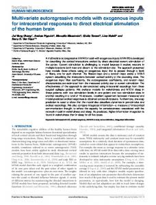
Figure 1: Method for approximating the trade-off curve between two convex objectives.

on a statistical analysis of the probability of errors in the topology (see also Yuan and Lin, 2007; Banerjee et al., 2008). Asadi et al. (2009) consider γ as a random variable and use a maximum a posteriori probability (MAP) estimation to choose γ and the covariance matrix. In the examples of this section we will use the following method for selecting γ. We first compute the entire trade-off curve between the two terms in the objective of (21), that is, between the log-likelihood and the penalty function h∞ (D(X)). The trade-off curve can be computed by solving (21) for a number of different values of γ (see below). We collect the topologies of the solutions along the trade-off curve, and solve the ML problem (16) for each of these topologies. We then rank the models using the Bayes information criterion (BIC), as discussed at the beginning of Section 3, and select the model with the lowest score. In this approach, the convex heuristic is used as a preprocessing step to reduce the number of topologies that are examined using the BIC, and to filter out topologies that are unlikely to be competitive. 4.1.2 T RACING T RADE - OFF C URVES The trade-off curves are computed by solving (21) for a sequence of values of γ. To obtain an accurate estimate of the curve with only a small number of values γ we use a method which is illustrated in Figure 1 for a generic trade-off between two convex cost functions f1 and f2 . We first solve the scalarized problem minimize

f1 (x) + γ f2 (x)

(31)

for two positive values γ1 , γ2 near the opposite ends of the trade-off curve. This gives the points labeled 1 and 2 on the trade-off curve. The values of γ1 and γ2 also define the slopes of straight lines that support the trade-off curve at points 1 and 2. Since the trade-off curve is convex, we can conclude that the curve between 1 and 2 lies somewhere in the shaded triangular region. As γ3 , we choose the value that corresponds to the slope of the straight line between 1 and 2. Solving problem (31) with γ = γ3 gives point 3 on the trade-off curve and a straight line that supports the curve at point 3. The trade-off curve between points 1 and 2 is now known to lie in the union of the two shaded triangles. Next, we solve the problem (31) for a value γ4 corresponding to the slope of the straight line between points 1 and 3, and a value γ5 corresponding to the slope of the straight line between 3 and 2. In this example, we obtain fairly accurate upper and lower bounds of the actual trade-off curve after solving five scalarized problems (31). 2683


4.1.3 T HRESHOLDING With a proper value of γ, the regularized ML problem (21) has a sparse solution Y , resulting in a sparse inverse spectrum S(ω)−1 . When solved with a limited accuracy, the entries of Y are not exactly zero. We will use the following method to determine the topology from the computed solution. We calculate the inverse spectrum S(ω)−1 and normalize it by scaling its rows and columns so that the diagonal is one: R(ω) = diag(S(ω)−1 )−1/2 S(ω)−1 diag(S(ω)−1 )−1/2 . The normalized inverse spectrum R(ω) is known as the partial coherence (Brillinger, 1981; Dahlhaus, 2000). Its entries are between 0 and 1 in magnitude, and measure the conditional dependence between the corresponding variables, after removing the linear effects from the other variables. In the static case (p = 0), R(ω) reduces to the normalized concentration matrix. To estimate the graph topology we compare the L∞ -norms of the entries of R(ω), ρi j = sup |R(ω)i j | ω

with a given threshold. This thresholding step is similar to thresholding in other sparse methods, for example the thresholded lasso and Dantzig estimators in Lounici (2008). To simplify the interpretation we will use the same threshold value (10−1 ) in all the experiments, that is, we remove edge (i, j) from the graph if ρi j ≤ 10−1 . 4.2 Experiment 1 In the first series of experiments we generate AR models with sparse inverse spectra by setting B0 = I and randomly choosing sparse lower triangular matrices Bk with entries ±0.5. The random trials are continued until a stable AR model is found. The AR process is then used to generate N samples of the time series. The model dimensions are n = 20 and p = 2. 4.2.1 T OPOLOGY S ELECTION We first illustrate the basic topology selection method outlined above using the correct model order (p = 2). The sample size is N = 512. Figure 2 shows the trade-off curve between the penalty h∞ (D(X)) and the log-likelihood L (X). We calculate the inverse spectra (10) for the computed points on the trade-off curve, and apply a threshold to them (as explained above, by setting entries with ρi j ≤ 10−1 to zero). The resulting topologies are shown in Figure 3. The patterns range from quite dense (small γ) to very sparse (large γ). The sparsity of the densest solution (γ = 10−5 ) is identical to the sparsity of the leastsquares estimate (i.e., the solution of the equations (15) with C given in (13) or, equivalently, the ML solution of (12) without the sparsity constraints). For each of the nine sparsity patterns, we solve the ML problem subject to sparsity constraints (16). We rank the nine solutions using the AICc and BIC scores defined in (20). Figure 4 shows the two scores and the negative log-likelihood as functions of γ. The models that minimize the AICc /BIC scores turn out to be the same in this example (the models for γ = 0.15) and the corresponding topology is shown in Figure 5 (left). Only seven entries are misclassified (six entries are misclassified as zeros; one as nonzero). The sparsity pattern in the middle is the topology estimated by thresholding the partial coherence spectrum of 2684


−18

−20

L (X)

−22

−24

−26

−28 0

10

20

30

40

50

60

70

h∞ (D(X)) Figure 2: Trade-off curve between the log-likelihood L (X) and h∞ (D(X)).

γ = 0.00

γ = 0.02

γ = 0.04

5

5

5

10

10

10

15

15

15

20

20 10

20

20 10

γ = 0.08

20

10

γ = 0.15

γ = 0.26

5

5

5

10

10

10

15

15

15

20

20 10

20

20 10

γ = 0.47

20

10

γ = 0.85 5

5

10

10

10

15

15

15

20 10

20

20

γ = 2.00

5

20

20

20 10

20

10

20

Figure 3: Topologies of solutions along the tradeoff curve in Figure 2 (ordered from right to left on the tradeoff curve).

2685


28

26

24

22

AICc BIC −L

20

18 0

0.5

1

γ

1.5

2

Figure 4: AICc and BIC scores, and maximized log-likelihood for solutions on the trade-off curve in Figure 2.

the least-squares solution with the correct model order (p = 2). This pattern is computed by solving the ML problem (12) without constraints, and then thresholding the partial coherence (using the same threshold value 0.1 as in the other experiments). The difference between the two patterns clearly shows the benefits of the nonsmooth regularization for estimating a sparse topology. The sparsity pattern on the right of Figure 5 is obtained from the covariance selection method with ℓ1 norm regularization (i.e., by setting p = 0 in the regularized ML problem (21)) and thresholding the partial coherence. Ignoring the model dynamics substantially increased the error in the topology selection. 4.2.2 C OMPARISON

WITH

OTHER T YPES OF R EGULARIZATION

To compare the quality of the sparse models with the models obtained from other estimation methods we evaluate the Kullback-Leibler (KL) divergence (Bach and Jordan, 2004) between the true and the estimated spectra as a function of the sample size N for the following six methods. 1. ML estimation without conditional independence constraints (or least-squares estimate). This is the solution of (12) without the constraints, and it can be computed by solving the normal equations (15). 2. ML estimation with conditional independence constraints determined by thresholding the partial coherence matrix of the least-squares estimate (solution 1). 3. ML estimation with Tikhonov regularization and without conditional independence constraints. Tikhonov regularization (also known as ridge regression or ℓ2 -regularization) is widely used in statistics and estimation (Hastie et al., 2009, §3.4). A Tikhonov-regularized ML estimate 2686


0

0

0

2

2

2

4

4

4

6

6

6

8

8

8

10

10

10

12

12

12

14

14

14

16

16

16

18

18

18

20

20

0

2

4

6

8

10 12 14 16 18 20

0

20 2

4

6

8

10 12 14 16 18 20

0

2

4

6

8

10 12 14 16 18 20

Figure 5: Left. The sparsity pattern from the regularized ML problem with γ = 0.15. Middle. The sparsity pattern estimated from the least-squares solution. Right. The sparsity pattern from the regularized ML problem for a static model (p = 0). The blue squares are the correctly identified nonzero entries (true positives). The red circles are the entries that are misclassified as nonzero (false positives). The black crosses are entries that are misclassified as zeros (false negatives).

is the solution of minimize −2 log det B0 + tr(CBT B) + γkBk2F . The solution can be computed from the normal equations (15) with C replaced by C + γI. The solution of this problem can therefore also be viewed as a ML estimate using a perturbed sample covariance matrix C + γI. In the experiment, the value of γ is determined by performing a five-fold cross-validation (Hastie et al., 2009, §7.10). 4. ML estimation with conditional independence constraints determined by thresholding the inverse spectral density for the Tikhonov estimate (solution 3). 5. Regularized ML estimation with h∞ -penalty. This is the solution of problem (21) with penalty function (22). 6. ML estimation with conditional independence constraints determined by thresholding the inverse spectral density for the h∞ -regularized ML estimate (solution 5). The total number of variables in this example is n(n + 1)/2 + pn2 = 1010 variables. We show the results in Figure 6 in two different settings: with small sample sizes (N < 1010) and with moderate to large sample sizes (N ≥ 1010). We can note that for small sample sizes N the constrained ML estimates (models 2,4,6) are not better than the unconstrained estimates (models 1,3,5), and much worse in the case of the Tikhonov-regularized estimates. This can be explained by large errors in the estimated topology. For larger N the constrained estimates are consistently better than the unconstrained models, and for very large N the three constrained ML estimates give the same accuracy. For small and moderate N we also see that model 6 (ML estimate for the topology selected via nonsmooth regularization) is much more accurate than the other methods. 2687


Small sample sizes 7

1 2

(1) LS (2) LS+Constrained MLE (3) Tikhonov (4) Tikhonov+Constrained MLE (5) L1 Regularization (6) L1+Constrained MLE

6

KL divergence

5

4

4 3 2 3

1 0

6

5

128

256

512

N Moderate to large sample sizes 0.35

1

(1) LS (2) LS+Constrained MLE (3) Tikhonov (4) Tikhonov+Constrained MLE (5) L1 Regularization (6) L1+Constrained MLE

0.3 3

KL divergence

0.25 0.2 0.15

2

4 5

0.1 6

0.05 0

1024

2048

4096

8192

16384

N Figure 6: KL divergence between estimated AR models and the true model (n = 20, p = 2) versus the number of samples N. We compare six methods: (1) least-squares estimate, (2) constrained ML estimate with topology estimated by thresholding solution 1, (3) ML estimate with Tikhonov regularization, (4) constrained ML estimate with topology estimated by thresholding solution 3, (5) regularized ML estimate with h∞ -penalty, (6) constrained ML estimate with topology estimated by thresholding solution 5. 2688


4.2.3 E RRORS IN T OPOLOGY AS A F UNCTION OF S AMPLE S IZE In the last figure (Figure 7) we examine how fast the error in the topology selection decreases with increasing sample length N for three topology selection methods: LS estimation followed by thresholding, ML estimation with Tikhonov regularization followed by thresholding, and ML estimation with nonsmooth regularization followed by thresholding. For each sample size N we show the errors averaged over 50 sample sequences (i.e., 50 different sample covariance matrices C). “False positives” refers to entries that are incorrectly classified as nonzeros (i.e., incorrectly added edges in the graphical model). “False negatives” are entries that are incorrectly classified as zeros (i.e., incorrectly deleted edges). The top graphs in Figure 7 show the fraction of false positives and false negatives versus the sample size. The bottom graphs show the total fraction of misclassified entries. We compare the three methods listed above. As can be seen, the total error in the estimated topology is reduced in the regularized estimates, and the errors decrease more rapidly when we regularize with the sum-of-norms penalty h∞ . 4.3 Experiment 2 In the second experiment we compare different penalty functions h for the regularized ML problem (21): the ‘sum-of-ℓ∞ -norms’ penalty h∞ defined in (22), the ‘sum-of-ℓ2 -norms’ penalty h2 defined in (28) with α = 2, and the ‘sum-of-ℓ1 -norms’ penalty h1 defined in (28) with α = 1. These penalty functions all yield models with a sparse inverse spectrum S(ω)−1 = Y0 +

1 p −jkω ∑ (e Yk + ejkωYkT ), 2 k=1

but have different degrees of sparsity for the entries (Yk )i j within each group i, j. The data are generated by randomly choosing sparse coefficients Yk of an inverse spectrum (10). For each (i, j) of nonzero locations in S(ω)−1 , we select random values (Yk )i j with about the same magnitude for all k. If necessary, a multiple of the identity matrix is added to Y0 to guarantee the positiveness of the spectrum. An AR realization of the spectrum is then computed by spectral factorization and used to generate sample time series. The model dimensions are n = 5, p = 7. Figure 8 shows typical values for the estimated coefficients (Yk )i j . The three penalty functions all give the same topology, but a different sparsity with the same group i, j of coefficients. The sparsity within each group is largest for the h1 -penalty and smallest for the h∞ -penalty. Table 1 shows the results of topology selection with the three penalties, for sample size N = 512 and averaged over 50 sample sequences. The h∞ -penalty gives the models with the smallest KL divergence and smallest error in topology. This is to be expected, given the distribution of the nonzero coefficients (Yk )i j in the AR models that were used to generate the data. The results also agree with a comparison of different norms in a composite penalty function (Zhao et al., 2009). In general the best choice of norm will depend on how the coefficients are distributed within each group.

5. Applications This section presents two examples of real data sets to demonstrate how topology selection can facilitate studies of relationship in multivariate time series. 2689


Fraction of false positives

Fraction of false negatives

1

0.35

L1 LS Tikhonov

0.8

0.3

L1 LS Tikhonov

0.25

0.6

0.2 0.15

0.4

0.1

0.2 0.05

0

128

256

512

1024

2048

0

4096

N

128

256

512

1024

2048

4096

N Total error

0.9 0.8

L1 LS Tikhonov

0.7 0.6 0.5 0.4 0.3 0.2 0.1 0

128

256

512

1024

2048

4096

N Figure 7: Top left. Fraction of incorrectly added edges in the estimated graph (number of upper triangular nonzeros in the estimated pattern that are incorrect, divided by the number of upper triangular zeros in the correct pattern). Top right. Fraction of incorrectly removed edges in the estimated graph (number of upper triangular zeros in the estimated pattern that are incorrect, divided by the number of upper triangular nonzeros in the correct pattern). Bottom. The combined classification error computed as the sum of the false positives and false negatives divided by the number of upper triangular entries in the pattern.

5.1 Functional Magnetic Resonance Imaging (fMRI) Data In this section we apply the topology selection method to a functional magnetic resonance imaging (fMRI) time series. We use the StarPlus fMRI data set1 (Mitchell et al., 2004), which was analyzed 1. StarPlus data can be found at www.cs.cmu.edu/afs/cs.cmu.edu/project/theo-81/www/.

2690


(i, j) = (4, 1)

|(Yk )i j | (h1 )

(i, j) = (2, 1) 0.4

0.4

0.4

0.4

0.2

0.2

0.2

0.2

0

0

k

1 2

0

k

k

1.5

1.5

1

1

1

1

0.5

0.5

0.5

0.5

3

0

0

k |(Yk )i j | (h∞ )

4

0

k 1.5

|(Yk )i j | (h2 )

1.5

5

(i, j) = (5, 4)

(i, j) = (5, 2)

0

k

0

k

k

0.4

0.4

0.4

0.4

0.3

0.3

0.3

0.3

0.2

0.2

0.2

0.2

0.1

0.1

0.1

0.1

0

0

0

k

k

0

k

k

Figure 8: Nonzero coefficients |(Yk )i j | for regularized ML estimates with penalty hα , for α = 1, 2, ∞.

Dimensions n = 20, n = 20, n = 30, n = 30,

p=2 p=4 p=2 p=4

KL divergence h1 h2 h∞ 0.24 0.22 0.21 0.33 0.24 0.19 0.40 0.35 0.30 0.59 0.46 0.40

Error in topology (%) h1 h2 h∞ 11.8 11.9 11.6 1.65 1.19 0.51 9.95 8.83 7.96 5.18 3.97 3.53

Table 1: Accuracy of topology selection methods with penalty hα for α = 1, 2, ∞. The table shows the average KL divergence with respect to the true model and the average percentage error in the estimated topology (defined as the sum of the false positives and false negatives divided by the number of upper triangular entries in the pattern), averaged over 50 instances.

using covariance selection in Scheinberg and Rish (2009). The data consists of 80 time series (runs) of brain image scans. In half of the 80 runs the input stimulus shown to the subject is a picture; in the other half it is a sentence. Each run contains 16 images, resulting in 640 images for each input. Mitchell et al. (2004) suggest a region of interest (ROI) of 1718 voxels. To reduce the dimension we took averages over groups of voxels in the ROI and considered four reduced graphs with n = 7, 50, 100, and 190 nodes, respectively. We fit two different AR models, one for each input. The AR model orders selected by the BIC are shown in Table 2. As the problem size (n) becomes larger, the BIC tends to pick a static model 2691


Input Picture Sentence

n=7 p=1 p=1

n = 50 p=1 p=1

n = 100 p=0 p=0

n = 190 p=0 p=0

Table 2: AR model orders for the fMRI data set. Input Picture Sentence

Static models (p = 0) ℓ1 Tikhonov LS 991 4116 4203 922 4021 4131

Time series models (p = 1) ℓ1 Tikhonov LS 0 13467 13465 0 13240 13238

Table 3: Relative BIC scores of six models fitted to two fMRI time series of size n = 50. The ‘static’ models are Gaussian graphical models (i.e., AR models of order p = 0), the time series models are AR models of order p = 1. The models are constrained ML estimates with topologies estimated using three different methods: Regularized ML estimate with hα -penalty, Tikhonov-regularized ML estimate, and the least-squares estimate. The BIC scores are relative to the score of the best model (time series models of regularized ML estimate with hα -penalty).

1

1

0.9

0.9

0.8

0.8

0.7

0.7 L1−static

0.6

Density

Density

L1−static L1−ts

0.5

Tikhonov−static

0.4

Tikhonov−ts

0.6

L1−ts

0.5

Tikhonov−static Tikhonov−ts

0.4

LS−static

LS−static 0.3

0.3

LS−ts

0.2

0.2

0.1

0.1

0

7

50

100

n

190

0

LS−ts

7

50

100

n

190

Figure 9: Density of the graphical models of fMRI data for ‘picture’ stimulus (left) and for ‘sentence’ stimulus (right). The density is computed as the number of nonzero entries in the estimated inverse spectrum divided by n2 .

(p = 0). Table 3 shows the BIC scores of different models for the experiment with size n = 50. The topologies selected by the BIC are the regularized ML estimates with h∞ -penalty. Figure 9 shows the sparsity of the estimated graphs from the least-squares, Tikhonov-regularized ML, and h∞ -regularized ML methods. The plots show that the h∞ -regularization produces much sparser graphs than the other two methods. To get an idea of the accuracy of the estimated network structure, we validated the result with a simple classification experiment. For each input we keep one fMRI run as a test problem and use 2692


model order p=0 p=1

n=7 0.21 0.20

n = 50 0.16 0.16

n = 100 0.11 0.16

n = 190 0.06 0.11

Table 4: Classification error of fMRI data versus model size. The error is the number of runs for which the stimulus input is correctly identified divided by the total number of runs (40).

the 39 remaining runs to estimate a sparse AR model. The two models are then used to guess the inputs shown to the subject during the test run. The classification algorithm computes the likelihood of each input, based on the two models, and selects the input with the highest likelihood. We repeat this for each of the 40 choices of test run. Table 4 shows the classification error versus the number of nodes in the graph. We see that the classification is quite successful and achieves an error in the range 6–20%. The error tends to be smaller if we use less averaging (larger n). We also note that for each n, the AR model of order p chosen in Table 2 also performs slightly better in the classification experiment. 5.2 International Stock Market Data We consider a multivariate time series of 17 stock market indices: the S&P 5000 composite index (U.S.), Toronto stock exchange 300 index (Canada), the All ordinary composite stock index (Australia), the Nikkei 225 stock index (Japan), the Hang Seng stock composite index (Hong Kong), the FTSE 100 share index (United Kingdom), the Frankfurt DAX 30 composite index (German), the CAC 40 stock composite index (France), MIBTEL index (Italy), the Zurich Swiss Market composite index (Switzerland), the Amsterdam exchange index (Netherlands), the Austrian traded index (Austria), IBEX 35 (Spain), BEL 20 (Belgium), the OMX Helsinki 25 index (Finland), the Portugese stock index (Portugal), the Irish stock exchange index (Ireland). The data were stock index closing prices recorded from June 3, 1997 to June 30, 1999 and obtained from www.globalfinancialdata.com. The data were converted to US dollars. Missing data due to national holidays were replaced by the most recent values. For each market we use as variable the return between trading day k − 1 and k, defined as rk = 100 log(πk /πk−1 ), where πk is the closing price on day k. This results in 17-dimensional time series of length 540. Similar time series for a smaller number of markets were analyzed in Bessler and Yang (2003) and Abdelwahab et al. (2008). We solve the h∞ -regularized ML problem with model orders ranging from p = 0 to p = 3, and for each value collect the topologies along the trade-off curve, as in the previous examples. The AICc and BIC criteria were then used to select a model. Both criteria selected a model of order p = 1 and the same sparsity pattern (corresponding to a value γ = 0.34). Figure 10 (right) shows ρi j , the maximum magnitude of the partial coherence of the model, and compares it with a thresholded nonparametric estimate obtained with Welch’s method (Proakis, 2001) and the constrained ML model with topology obtained by thresholding the least-squares estimate. We note that the graph topologies suggested by the nonparametric and least-squares estimates are much denser than the regularized ML estimate. 2693


2

2

2

4

4

4

6

6

6

8

8

8

10

10

10

12

12

12

14

14

14

16

16

2

4

6

8

10

12

14

16

16

2

4

6

8

10

12

14

16

2

4

6

8

10

12

14

16

Figure 10: The maximum magnitude ρi j of the partial coherence for three models of the stock exchange data. Left: Thresholded nonparametric sample estimate using Welch’s method. Middle: Constrained ML estimate with topology determined from the LS solution. Right: Constrained ML estimate with topology determined from the h∞ -regularized ML estimate.

Figure 11 shows the graphical model estimated by the h∞ -regularized ML problem. The thickness of the edges is proportional to ρi j . We recognize many connections that can be explained from geographic proximity or economic ties between the countries. For example, we see strong connections between the U.S. and Canada, between Australia, Japan, and Hong Kong, between Hong Kong and U.K., between the southern European countries, et cetera. Overall the graphical model seems plausible, and the experiment suggests that the topology selection method is quite effective.

6. First-order Optimization Algorithms In the preceding sections we have considered four convex optimization problems. The constrained ML estimation problem (16) and its dual (17) have differentiable objectives and linear equality and matrix inequality constraints. The regularized ML problem (21) also includes a nondifferentiable term in the objective, and its dual (27) has a differentiable objective but constraints that involve nondifferentiable functions. These optimization problems can be solved by interior-point methods, for example, the path-following methods developed for convex determinant maximization problems (Toh, 1999; Vandenberghe et al., 1998). In practice, however, the problems are often too large for interior-point methods because they involve matrix variables (X or Z) of high dimension. In this section we therefore investigate less expensive first-order algorithms applied to a reformulation of the dual problems (17) and (27). The dual approach avoids several difficulties that arise in first-order methods applied to the primal problems: the complicated constraints in the constrained ML problem (16), the fact that its objective, which is also the first term in the objective of the regularized ML problem (21), is not strictly convex, the nondifferentiability of the penalty term in (21), and, most important, the fact the solution X has low rank and therefore lies on the boundary of the feasible set. (For the regularized ML problem (21), these difficulties could be addressed as in the covariance selection method of Banerjee et al. (2008), by applying Nesterov’s fast gradient method to an approximation of the primal problem with a smoothed objective and a closed bounded constraint set (Nesterov, 2005). In our limited experience, with a fixed and conservative choice of 2694


AU

JP

US CA IR

AT

HK UK

FN FR

ρi j (0, 0.15) [0.15 , 0.25) [0.25 , 0.35) [0.35 , 0.45) [0.45 , 0.55) [0.55 , 0.65) [0.65 , 0.75)

BE

PO

GE NE CH

IT SP

Figure 11: A graphical model of stock market data. The strength of connections is represented by the width of the blue links, which is proportional to ρi j = supω |R(ω)i j | if it is greater than 0.15.

the smoothing and bounding parameters, this algorithm was slower than the dual gradient projection method described in this section, so we will not pursue it here.) 6.1 Reformulated Dual Problems To reformulate the dual problems we eliminate the variable W in (17) and (27). Let V = C + T(P(Z)), respectively, V = C + T(Z). The inequality V−

W 0

0 0

=

T V00 −W V1:p,0 V1:p,0 V1:p,1:p

0,

is equivalent to V1:p,1:p 0,

range(V1:p,0 ) ⊆ range(V1:p,1:p ),

† T V1:p,1:p V1:p,0 W, V00 −V1:p,0

(32)

† where V1:p,1:p is the pseudo-inverse of V1:p,1:p . If V 0, then the matrix W with maximum deterT V† minant that satisfies (32) is equal to V00 −V1:p,0 1:p,1:pV1:p,0 , the Schur complement of V1:p,1:p in V . This observation allows us to eliminate W from (17) and (27). Problem (17) can be written as an unconstrained problem maximize −φ(C + T(P(Z))), (33)

2695


and problem (27) as a problem with simple constraints maximize −φ(C + T(Z)) p

∑ (|(Zk )i j | + |(Zk ) ji |) ≤ γ,

subject to

i 6= j

k=0

diag(Zk ) = 0,

(34)

k = 0, . . . , p.

Here φ : Sn(p+1) → R is defined as † T φ(V ) = − log det V00 −V1:p,0 V1:p,1:p V1:p,0 − n, n(p+1)

with domain dom φ = {V ∈ S+ can be expressed as

T V† | V00 −V1:p,0 1:p,1:pV1:p,0 ≻ 0}. This function is convex, since it

φ(V ) = inf − log detW

W 0

0 0

V

− n,

and convexity of this expression follows from results in convex analysis (Boyd and Vandenberghe, 2004, §3.2.5). It is also a smooth function on the interior of its domain and its gradient at a positive definite V can be expressed as 0 0 −1 ∇φ(V ) = −V + . (35) −1 0 V1:p,1:p T V −1 V This can be seen, for example, from the identity detV = detV1:p,1:p det(V00 − V1:p,0 1:p,1:p 1:p,0 ), which gives φ(V ) = − log detV + log detV1:p,1:p − n, and the fact that the gradient of log det X is X −1 . If V = C +T(P(Z)) ≻ 0 at the optimum of (33) then the primal optimal solution can be computed from Z via the expressions

X =V

−1

−

0 0 −1 0 V1:p,1:p

=

−I −1 V1:p,1:p V1:p,0

W

−1

−I −1 V1:p,1:p V1:p,0

T

(36)

T V −1 V where V = C + T(P(Z)) and W = V00 − V1:p,0 1:p,1:p 1:p,0 . The expression for X follows from the optimality condition (18) and the identities

V=

V

−1

=

T V −1 V V00 −V1:p,0 1:p,1:p 1:p,0 0 0 0

0 0 −1 0 V1:p,1:p

+

−I −1 V1:p,1:pV1:p,0

T V −1 V1:p,0 1:p,1:p I

+

−1 T (V00 −V1:p,0 V1:p,1:p V1:p,0 )−1

V1:p,1:p

T V −1 V1:p,0 1:p,1:p I

T

−I −1 V1:p,1:pV1:p,0

,

T

.

(37)

The formula for V −1 also provides an alternative form of the gradient (35). Similarly, if C + T(Z) ≻ 0 at the optimum of (34) then the primal optimal X can be computed from (36) with V = C + T(Z). The reformulated dual problems are interesting because they can often be solved by gradient algorithms for unconstrained optimization or gradient projection algorithms for problems with simple constraints. To explain this, we again distinguish between Toeplitz and non-Toeplitz C. If C is 2696


block-Toeplitz, then it can be shown that the functions φ(C + T(P(Z))) and φ(C + T(Z)) are closed convex functions (i.e., with closed sublevel sets) and that their domains are open. Consider the function φ restricted to the set of block-Toeplitz matrices, that is, φ(T(R)), where R ∈ Mn,p . By definition, R is in the domain of φ(T(R)) if T(R) 0 and there exists a positive definite W with W 0 T(R) . 0 0 From the property of block-Toeplitz matrices mentioned in Section 2.3, this implies T(R) ≻ 0. In other words, the domain of φ(T(R)) is the open set {R | T(R) ≻ 0}. By a similar argument, if a sequence of matrices R in the domain of φ(T(R)) converges to a point R¯ in the boundary of the ¯ 1:p,1:p in T(R) ¯ must be singular, and hence φ(T(R)) → domain, then the Schur complement of T(R) ∞. For a continuous function with an open domain this is equivalent to closedness (Boyd and Vandenberghe, 2004, p.639). If C is not block-Toeplitz, then the functions φ(C +T(P(Z))) and φ(C +T(Z)) are not necessarily closed, and their domains not necessarily open. One implication is that it is possible that the optimal solution of (33) or (34) is at a point in the boundary of the domain of the cost function, that is, a point where C + T(P(Z)) or C + T(Z) are singular. However in practice, C is usually approximately block-Toeplitz and one can expect that the functions are often closed. Moreover, in order to apply unconstrained minimization algorithms it is sufficient that the algorithm is started at a point Z (0) for which the sublevel set {Z | φ(C + T(P(Z))) ≤ φ(C + T(P(Z (0) )))} is closed. This condition is considerably weaker than the requirement that all sublevel sets are closed. 6.2 Gradient Projection Algorithms We now present some details on first-order algorithms for the reformulated dual problems. We focus on the constrained problem (34) since the unconstrained problem (33) can be handled as a special case. We first describe a version of the classical gradient projection with a backtracking line search (Polyak, 1987; Bertsekas, 1999). To simplify the notation we will use a generic problem format minimize f (x) subject to x ∈ C where f : Rn → R is convex and continuously differentiable with an open domain, and C is a closed convex set. We assume that a feasible point x(0) is known and that the sublevel set

S = {x ∈ dom f ∩ C | f (x) ≤ f (x(0) )} is closed and bounded. The closedness assumption is satisfied if f is a closed function. (See the previous paragraph on the validity of this assumption for problems (33) and (34).) We assume that projections on C are inexpensive and we denote the projection operator by P :

P (y) = argmin kx − yk2 . x∈C

The gradient map associated with f and C is defined as Gt (x) =

1 (x − P (x − t∇ f (x))) t

for t > 0. For an unconstrained problem, the gradient map is Gt (x) = ∇ f (x), independent of t. 2697


6.2.1 BASIC G RADIENT P ROJECTION The basic gradient projection method starts at x(0) and continues the iteration x(k) = P x(k−1) − tk ∇ f (x(k−1) ) = x(k−1) − tk Gtk (x(k−1) )

(38)

until a stopping criterion is satisfied. A classical convergence result states that x(k) converges to an optimal solution if tk is fixed and equal to 1/L, where L is a constant that satisfies k∇ f (u) − ∇ f (v)k2 ≤ Lku − vk2

∀u, v ∈ S ,

(39)

(Polyak, 1987, §7.2.1). Although our assumptions (S is closed and bounded, and dom f is open) imply that the Lipschitz condition (39) holds for some constant L > 0, its value is not known in practice, so the fixed step size rule tk = 1/L cannot be used. We therefore determine tk using a backtracking search (Beck and Teboulle, 2009). The step size search algorithm in iteration k starts at a value tk := t¯k where T s s t¯k = min T ,tmax , (40) s y where s = x(k−1) − x(k−2) ,

y = ∇ f (x(k−1) ) − ∇ f (x(k−2) ),

and tmax is a positive constant. (In the first iteration we initialize the step size as t1 = tmax .) The search then repeats the update tk := βtk (where β ∈ (0, 1) is an algorithm parameter) until x(k−1) − tk Gtk (x(k−1) ) ∈ dom f and tk f (x(k−1) − tk Gtk (x(k−1) )) ≤ f (x(k−1) ) − tk ∇ f (x(k−1) )T Gtk (x(k−1) ) + kGtk (x(k−1) )k22 . 2

(41)

The resulting step size tk is used in the update to x(k) in (38). Note that the trial points x(k−1) − tk Gtk (x(k−1) ) = P x(k−1) − tk ∇ f (x(k−1) )

generated during the step size search are not necessarily on a straight line. The trajectory is sometimes referred to as the projection arc (Bertsekas, 1999, §2.3). The step length ksk22 /sT y is known as the Barzilai-Borwein step size and forms the basis of spectral gradient methods (Barzilai and Borwein, 1988; Birgin et al., 2003; Figueiredo et al., 2007; Wright et al., 2009). It can be motivated by the easily established fact that ksk22 /sT y ≥ 1/L if f satisfies (39), so it is a readily computed upper bound for 1/L. 6.2.2 VARIATIONS The basic gradient projection method can be varied in several ways, some of which will be compared in the numerical experiments below. To avoid computing a projection for each trial step size tk in the step size search, we can replace the gradient update with x(k) = x(k−1) − tk Gt¯k (x(k−1) ) 2698

(42)


where t¯k is held fixed at the value (40) and tk is determined by a backtracking search: we take tk := t¯k and then backtrack (tk := βtk ) until x(k−1) − tk Gt¯k (x(k−1) ) ∈ dom f and tk f (x(k−1) − tk Gt¯k (x(k−1) )) ≤ f (x(k−1) ) − tk ∇ f (x(k−1) )T Gt¯k (x(k−1) ) + kGt¯k (x(k−1) )k22 . 2

(43)

In this method the trial points during the step size selection follow a straight line, and each step only requires a function evaluation. Many alternatives to the step size rules (38) and (42) are available in the literature, for example, the Armijo rule (Bertsekas, 1999, §2.3), and conditions that allow non-monotone convergence (Birgin et al., 2000; Lu and Zhang, 2009). In our experiments these variations gave similar results as the step size rules outlined above. Another attractive class of gradient projection algorithms are the optimal first-order methods originated by Nesterov (Nesterov, 2004; Tseng, 2008; Beck and Teboulle, 2009). For functions whose gradient is Lipschitz continuous on C , these p algorithms have a better complexity than the classical gradient projection method (at most O( 1/ε) iterations are needed to reach an accuracy ε, as opposed to O(1/ε) for the gradient projection method). These theoretical complexity results are valid if a constant step size tk = 1/L is used where L is the Lipschitz constant for the gradient, or if the step sizes form an nonincreasing sequence (tk+1 ≤ tk ) determined by a backtracking line search (Beck and Teboulle, 2009; Tseng, 2008). The assumption that the gradient is Lipschitz continuous on C does not hold for the problem considered here, and it is not clear if the convergence analysis can be extended to the case when the gradient is Lipschitz continuous only on the initial sublevel set. Nevertheless, an implementation with a backtracking line search worked well in our experiments (see next section). 6.2.3 I MPLEMENTATION D ETAILS The most important steps in the gradient projection algorithms applied to (33) are the evaluations of the gradient of the objective function and the projections on the set defined by the constraints. We now explain these two steps and the stopping criterion in more detail. The gradient (35) of φ at a point V can be evaluated from a Cholesky factorization V = LT L with L lower triangular. If we partition L as L00 0 L= L1:p,0 L1:p,1:p then ∇φ(V ) =

I −1 −L1:p,1:p L1:p,0

−1 −T L00 L00

I −1 −L1:p,1:p L1:p,0

T

.

The projection P (U) of a matrix U ∈ M p,n on the set defined by the constraints in (34) can be efficiently computed as follows. Clearly, the diagonal entries of P (U)k are zero for k = 0, . . . , p. To find the off-diagonal entries we can solve an independent problem p

minimize 2((Z0 )i j − (U0 )i j )2 + ∑ ((Zk )i j − (Uk )i j )2 + ((Zk ) ji − (Uk ) ji )2 p

subject to

k=1

∑ (|(Zk )i j | + |(Zk ) ji |) ≤ γ

k=0

2699


0

4

10

10 GP−line search GP−arc search Exact FISTA Modified FISTA

Relative error

10

10

−4

10

−6

0

10

−2

10

0

GP−line search GP−arc search Exact FISTA Modified FISTA

2

Duality gap

−2

10

200

400

600

800

1000

0

200

400

k

600

800

1000

k

Figure 12: Convergence of gradient projection algorithms. Left: Relative error ( f (Z (k) ) − f ⋆ )/| f ⋆ | versus the number of iterations. Right: Duality gap versus the number of iterations.

for each i, j with j > i. This is the problem of projecting a vector on the ℓ1 -norm ball. The solution is easily derived from duality and can be calculated by applying to the entries (Uk )i j the shrinkage operation familiar in sparse optimization (see, for example, Tibshirani, 1996). The following stopping criterion will be used in the experiments. At each iteration, we compute X in (36) from the current iterate Z. This matrix X is primal feasible, as can be seen from the identity (37) and the fact that C + T(Z) ≻ 0. By taking the Schur complement of (C + T(Z))1:p,1:p we also find a dual feasible W in (27). The duality gap between this primal feasible X and the dual feasible Z, W is η = − log det X00 + tr(CX) + γh(D(X)) − log detW − n = tr(CX) − n + γh(D(X))

= tr((C + T(Z))X) − n − tr(X T(Z)) + γh(D(X)) = − tr(X T(Z)) + γh(D(X)).

We terminate when the duality gap is below a given tolerance. 6.3 Numerical Example We generate AR models as in the experiment described in Section 4.2. In the first experiment, the model dimensions are n = 300, p = 2, N = 2n(p + 1). The true inverse spectrum has 10428 nonzero entries in the upper triangular part (a density of about 12%). The penalty parameter γ is set at γ = 0.1. The variable Z in the reformulated dual problem (34) is a matrix in M300,2 , so the problem has n(n + 1)/2 + pn2 = 225150 optimization variables. We start the gradient projection algorithm at a strictly feasible Z (0) = 0, and terminate when the duality gap is below 10−2 (the optimal value is on the order of hundreds). Figure 12 shows the relative error ( f (Z (k) ) − f ⋆ )/| f ⋆ | where f (Z) = φ(C + T(P(Z))) and f ⋆ is the optimal value. It also shows the duality gap η(k) versus the iteration number for a typical instance. ‘GP with arc search’ refers to the gradient projection method (38) with step size rule (41). 2700


4

Average CPU time (seconds)

10

3

10

2

10

1

GP with arc search

10

GP with line search

0

10

300

600

900

1200

1500

n(p + 1) Figure 13: Average CPU times (averaged over 10 runs) of the gradient projection algorithm versus the problem size. The algorithm stops when the duality gap is less than 10−1 . The red squares correspond to ‘GP with line search’ and the blue squares correspond to ‘GP with arc search’.

‘GP with line search’ refers to the gradient projection method (42) with step size rule (43). The step size searches required at most 15 backtracking steps to find an acceptable step size. As can be seen, a solution with a moderate accuracy (relative error in the range 10−4 –10−3 ) is obtained after a number of iterations that is only a fraction of the problem size. The convergence of the ‘arc search’ method is slightly faster, but it should be kept in mind that this method is more expensive than the ‘line search’. The ‘Exact FISTA’ method is the gradient projection algorithm with backtracking line search from Beck and Teboulle (2009) using monotonically decreasing step sizes (tk ≤ tk−1 , as required by the theory in Beck and Teboulle 2009). As can be seen the convergence was not faster than the classical gradient projection method. A heuristic modification in which the step sizes are not forced to be nonincreasing, but at each iteration the line searche is initialized at the Barzilai and Borwein steplength (40), was often about five times faster. This algorithm is referred to as ‘Modified FISTA’ in the figure. Figure 13 shows the CPU time versus problem size on a 3GHz Intel Pentium(R) 4 processor with 2.94 GB of RAM, for the ‘GP with arc search’ and ‘GP with line search’ algorithms. The test problems are generated as in the previous experiment, with p = 2 and varying n. The algorithms stop when it achieves a duality gap less than ε = 0.1. This yields a solution with a moderate accuracy (relative gap in the range 10−4 –10−3 ). The plot shows that the times needed to solving the regularized ML estimation using both algorithms are fairly comparable with a slight advantage for ‘GP with arc search’ when n is large. Although the backtracking steps in the arc search method are more expensive, the gradient projection method with this step size selection required fewer iterations in most cases. 2701


7. Conclusion We have presented a convex optimization method for topology selection in graphical models of autoregressive Gaussian processes. The method is based on augmenting the maximum likelihood estimation problem with an ℓ1 -type penalty function, chosen to promote sparsity in the inverse spectrum. By tracing the trade-off curve between the log-likelihood and the penalty function, we obtain a small set of sparse graph topologies, that can then be ranked according to information-theoretic criteria such as the AIC or BIC. This procedure avoids the combinatorial complexity of enumerating all possible topologies, and produces accurate results for smaller sample sizes than methods based on empirical or least-squares estimates. To solve the large, nonsmooth convex optimization problems that result from this formulation, we have investigated a gradient projection method applied to a reformulated dual problem. Experiments with randomly generated examples, and an analysis of an fMRI time series and a time series of international stock market indices were included to confirm the effectiveness of this approach.

Acknowledgments The authors thank Zhaosong Lu for interesting discussions on algorithms for the penalized ML problem. This research was supported by NSF under grant ECCS-0824003 and by a Royal Thai government scholarship.

References A. Abdelwahab, O. Amor, and T. Abdelwahed. The analysis of the interdependence structure in international financial markets by graphical models. International Research Journal of Finance and Economics, 15:291–306, 2008. N. Bani Asadi, I. Rish, K. Scheinberg, D. Kanevsky, and B. Ramabhadran. A MAP approach to learning sparse Gaussian markov networks. In IEEE International Conference on Acoustics, Speech and Signal Processing, pages 1721–1724, 2009. F. R. Bach and M. I. Jordan. Learning graphical models for stationary time series. IEEE Transactions on Signal Processing, 32:2189–2199, 2004. O. Banerjee, L. El Ghaoui, and A. d’Aspremont. Model selection through sparse maximum likelihood estimation for multivariate Gaussian or binary data. Journal of Machine Learning Research, 9:485–516, 2008. J. Barzilai and J. M. Borwein. Two-point step size gradient methods. IMA Journal of Numerical Analysis, 8:141–148, 1988. A. Beck and M. Teboulle. A fast iterative shrinkage-thresholding algorithm for linear inverse problems. SIAM Journal on Imaging Sciences, 2(1):183–202, 2009. D. P. Bertsekas. Nonlinear Programming. Athena Scientific, Nashua, New Hampshire, second edition, 1999. 2702


D.A. Bessler and J. Yang. The structure of interdependence in international stock markets. Journal of International Money and Finance, 22(2):261–287, 2003. E. G. Birgin, J. M. Mart´ınez, and M. Raydan. Nonmonotone spectral projected gradient methods on convex sets. SIAM J. on Optimization, 10(4):1196–1211, 2000. E. G. Birgin, J. M. Mart´ınez, and M. Raydan. Inexact spectral projected gradient methods on convex sets. IMA Journal of Numerical Analysis, 23:539–559, 2003. S. Boyd and L. Vandenberghe. Convex Optimization. Cambridge University Press, Cambridge, 2004. www.stanford.edu/˜boyd/cvxbook. D. R. Brillinger. Time series: Data analysis and theory. Holden-Day, San Francisco, California, expanded edition, 1981. J. Dahl, V. Roychowdhury, and L. Vandenberghe. Maximum-likelihood estimation of multivariate normal graphical models: large-scale numerical implementation and topology selection. Technical report, Electrical Engineering Department, UCLA, 2005. R. Dahlhaus. Graphical interaction models for multivariate time series. Metrika, 51(2):157–172, 2000. R. Dahlhaus, M. Eichler, and J. Sandkühler. Identification of synaptic connections in neural ensembles by graphical models. Journal of Neuroscience Methods, 77(1):93–107, 1997. A. P. Dempster. Covariance selection. Biometrics, 28:157–175, 1972. J. Duchi, S. Gould, and D. Koller. Projected subgradient methods for learning sparse Gaussians. In Proceeding of the Conference on Uncertainty in AI, 2008. M. Eichler. Fitting graphical interaction models to multivariate time serie. In Proceedings of the 22nd Conference on Uncertainty in Artificial Intelligence, 2006. M. Eichler. Testing nonparametric and semiparametric hypotheses in vector stationary processes. Journal of Multivariate Analysis, 99(5):968–1009, 2008. M. Eichler, R. Dahlhaus, and J. Sandkühler. Partial correlation analysis for the identification of synaptic connections. Biological Cybernetics, 89(4):289–302, 2003. S. Feiler, K.G. Müller, A. Müller, R. Dahlhaus, and W. Eich. Using interaction graphs for analysing the therapy process. Psychother Psychosom, 74(2):93–99, 2005. M. A. T. Figueiredo, R. D. Nowak, and S. J. Wright. Gradient projection for sparse reconstruction: Application to compressed sensing and other inverse problems. IEEE Journal of Selected Topics in Signal Processing, 1(4):586–597, 2007. R. Fried and V. Didelez. Decomposability and selection of graphical models for multivariate time series. Biometrika, 90(2):251–267, 2003. J. Friedman, T. Hastie, and R. Tibshirani. Sparse inverse covariance estimation with the graphical lasso. Biostatistics, 9(3):432, 2008. 2703


U. Gather, M. Imhoff, and R. Fried. Graphical models for multivariate time series from intensive care monitoring. Statistics in Medicine, 21(18):2685–2701, 2002. T. Hastie, R. Tibshirani, and J. Friedman. The Elements of Statistical Learning: Data Mining, Inference and Prediction. Springer, New York, 2nd edition, 2009. J. Z. Huang, N. Liu, M. Pourahmadi, and L. Liu. Covariance matrix selection and estimation via penalised normal likelihood. Biometrika, 93(1):85–98, 2006. Y. Kim, J. Kim, and Y. Kim. Blockwise sparse regression. Statistica Sinica, 16(2):375–390, 2006. S. L. Lauritzen. Graphical Models. Oxford University Press, Oxford, 1996. K. Lounici. Sup-norm convergence rate and sign concentration property of Lasso and Dantzig estimators. Electronic Journal of Statistics, 2:90–102, 2008. Z. Lu. Smooth optimization approach for sparse covariance selection. SIAM Journal on Optimization, 19:1807, 2009. Z. Lu. Adaptive first-order methods for general sparse inverse covariance selection. SIAM Journal on Matrix Analysis and Applications, 2010. forthcoming. Z. Lu and Y. Zhang. An augmented lagrangian approach for sparse principal component analysis. 2009. Submitted. N. Meinshausen and P. Bühlmann. High-dimensional graphs and variable selection with the Lasso. Annals of Statistics, 34(3):1436–1462, 2006. T.M. Mitchell, R. Hutchinson, R.S. Niculescu, F. Pereira, and X. Wang. Learning to decode cognitive states from brain images. Machine Learning, 57(1):145–175, 2004. Y. Nesterov. Introductory Lectures on Convex Optimization. Kluwer Academic Publishers, Dordrecht, The Netherlands, 2004. Y. Nesterov. Smooth minimization of non-smooth functions. Mathematical Programming Series A, 103:127–152, 2005. B. T. Polyak. Introduction to Optimization. Optimization Software, Inc., New York, 1987. J. Proakis. Digital Communications. McGraw-Hill, New York, fourth edition, 2001. R. Ravikumar, M. J. Wainwright, G. Raskutti, and B. Yu. High-dimensional covariance estimation by minimizing ℓ1 -penalized log-determinant divergence, 2008. URL http://www.citebase. org/abstract?id=oai:arXiv.org:0811.3628. Available from arxiv.org/abs/0811.3628. A. J. Rothman, P. J. Bickel, E. Levina, and J. Zhu. Sparse permutation invariant covariance estimation. Electronic Journal of Statistics, 2:494–515, 2008. R. Salvador, J. Suckling, C. Schwarzbauer, and E. Bullmore. Undirected graphs of frequencydependent functional connectivity in whole brain networks. Philosophical Transactions of the Royal Society B: Biological Sciences, 360(1457):937–946, 2005. 2704


K. Scheinberg and I. Rish. SINCO - a greedy coordinate ascent method for sparse inverse covariance selection problem. 2009. Submitted. J. Songsiri, J. Dahl, and L. Vandenberghe. Graphical models of autoregressive processes. In Y. Eldar and D. Palomar, editors, Convex Optimization in Signal Processing and Communications. Cambridge University Press, Cambridge, 2009. P. Stoica and R. L. Moses. Introduction to Spectral Analysis. Prentice Hall, London, 1997. R. Tibshirani. Regression shrinkage and selection via the Lasso. Journal of the Royal Statistical Society. Series B (Methodological), 58(1):267–288, 1996. J. Timmer, M. Lauk, S. Häußler, V. Radt, B. Köster, B. Hellwig, B. Guschlbauer, C.H. Lücking, M. Eichler, and G. Deuschl. Cross-spectral analysis of tremor time series. Internation Journal of Bifurcation and Chaos in applied Sciences and Engineering, 10(11):2595–2610, 2000. K.-C. Toh. Primal-dual path-following algorithms for determinant maximization problems with linear matrix inequalities. Computational Optimization and Applications, 14:309–330, 1999. P. Tseng. On accelerated proximal gradient methods for convex-concave optimization. SIAM Journal on Optimization, 2008. Submitted. L. Vandenberghe, S. Boyd, and S.-P. Wu. Determinant maximization with linear matrix inequality constraints. SIAM J. on Matrix Analysis and Applications, 19(2):499–533, April 1998. S.J. Wright, R.D. Nowak, and M.A.T. Figueiredo. Sparse reconstruction by separable approximation. IEEE Transactions on Signal Processing, 57(7):2479–2493, 2009. M. Yuan and Y. Lin. Model selection and estimation in regression with grouped variables. Journal of the Royal Statistical Society: Series B Statistical Methodology, 68(1):49–67, 2006. M. Yuan and Y. Lin. Model selection and estimation in the Gaussian graphical model. Biometrika, 94(1):19, 2007. P. Zhao, G. Rocha, and B. Yu. The composite absolute penalties family for grouped and hierarchical variable selection. The Annals of Statistics, 37(6A):3468–3497, 2009.

2705

Topology Selection in Graphical Models of Autoregressive Processes

Topology Selection in Graphical Models of Autoregressive Processes

Suggest Documents

1 Graphical models of autoregressive processes

1 Graphical models of autoregressive processes

Bayesian Model Selection for Beta Autoregressive Processes

Order selection for vector autoregressive models

MULTISTEP PREDICTION IN AUTOREGRESSIVE PROCESSES

Order Selection of Autoregressive Processes using Bridge Criterion

Conditional Autoregressive Hilbertian processes

Conditional Autoregressive Hilbertian processes

Duality in Graphical Models

Graphical models in Macaulay2

Joint Graphical Models for Date Selection in Timeline Summarization

Multivariate autoregressive models with

Copula selection for graphical models in ... - Semantic Scholar

Spatially Varying Autoregressive Processes

Autoregressive Negative Binomial Processes - CiteSeerX

Phasetype distributions, autoregressive processes and

Graphical Models

Estimation and Simulation of Autoregressive Hilbertian Processes ...

recurrence properties of autoregressive processes ... - Project Euclid

Estimation in autoregressive models with Markov regime

Graphical models for composable finite Markov processes 1 ... - UCL

AUTOREGRESSIVE MODELS AND SYSTEM ...

Model Uncertainty in Panel Vector Autoregressive Models

Multivariate Threshold Autoregressive Models in Geodesy