Total Recall: Automatic Query Expansion with a Generative Feature ...

Total Recall: Automatic Query Expansion with a Generative Feature Model for Object Retrieval Ondˇrej Chum1 , James Philbin1 , Josef Sivic1 , Michael Isard2 and Andrew Zisserman1 1 Visual Geometry Group, Department of Engineering Science, University of Oxford 2 Microsoft Research, Silicon Valley {ondra,james,josef,az}@robots.ox.ac.uk

Abstract

[email protected]

?

Given a query image of an object, our objective is to retrieve all instances of that object in a large (1M+) image database. We adopt the bag-of-visual-words architecture which has proven successful in achieving high precision at low recall. Unfortunately, feature detection and quantization are noisy processes and this can result in variation in the particular visual words that appear in different images of the same object, leading to missed results. In the text retrieval literature a standard method for improving performance is query expansion. A number of the highly ranked documents from the original query are reissued as a new query. In this way, additional relevant terms can be added to the query. This is a form of blind relevance feedback and it can fail if ‘outlier’ (false positive) documents are included in the reissued query. In this paper we bring query expansion into the visual domain via two novel contributions. Firstly, strong spatial constraints between the query image and each result allow us to accurately verify each return, suppressing the false positives which typically ruin text-based query expansion. Secondly, the verified images can be used to learn a latent feature model to enable the controlled construction of expanded queries. We illustrate these ideas on the 5000 annotated image Oxford building database together with more than 1M Flickr images. We show that the precision is substantially boosted, achieving total recall in many cases.

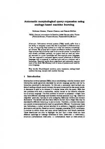
Figure 1. A sample of challenging results returned by our method in answer to a visual query for the Tom Tower, Christ Church College, Oxford (top left), which weren’t found by a simple bag-ofvisual-words method. This query was performed on a large dataset of 1,145,645 images.

vocabulary. The corpus is then summarized using an index where each image is represented by the visual words that it contains. At query time the system is presented with a query in the form of an image region. This region is itself processed to extract feature descriptors that are mapped onto the visual word vocabulary, and these words are used to query the index. The response set of the query is a set of images from the corpus that contain a large number of visual words in common with the query region. These response images may subsequently be ranked using spatial information to ensure that the response and the query not only contain similar features, but that the features occur in compatible spatial configurations [14, 17, 18, 20]. This procedure can be interpreted probabilistically as follows: the system extracts a generative model of an object from the query region; then forms the response set from those images in the corpus that are likely to have been gen-

1. Introduction The leading methods for object retrieval from large image corpora all rely on variants of the same technique [11, 12, 18]. First, each image in the corpus is processed to extract features in some high-dimensional descriptor space. These descriptors are quantized or clustered to map every feature to a “visual word” in some much smaller discrete 1

erated from that model. The generative model in this case is a spatial configuration of visual words extracted from the query region, together with a “background” distribution of words that encodes the overall frequency statistics of the corpus. In this paper we explore ways to derive better object models given the query region, in order to improve retrieval performance. We keep the form of the model fixed: it is still a configuration of visual words. However, rather than simply extracting the model from the single input query region, we enrich it with additional information from the corpus; we refer to this as a latent model of the object. This richer model achieves substantially better retrieval performance than the state of the art [12] on the Oxford Buildings dataset [2]. The latent model is a generalization of the idea of query expansion, a well-known technique from the field of textbased information retrieval [4, 16]. In text-based query expansion a number of the high ranked documents from the original response set are used to generate a new query that can be used to obtain a new response set. This is a form of blind relevance feedback [16] in that it allows additional relevant terms to be added to the query. It is particularly well suited to our problem domain for two reasons. First, the spatial structure of images allows us to be very robust to false positives. In text retrieval, relevance feedback attempts to construct a topic model of relevance based on terms in the documents. Due to the complexities of natural language, the relevant terms may be spread arbitrarily throughout the returned documents, and the task is complicated by the dramatic changes in meaning that can arise from subtle rearrangement of language terms. Consequently there is substantial danger of topic drift, where an incorrect model is inferred from the initial result set, leading to divergence as the process is iterated. In the image retrieval case we are greatly assisted by the fact that we can construct a model of a region rather than the whole image, and that the image data within the region is very likely to correspond to the object of interest. While there may be occlusions obscuring parts of some matching regions, it is reasonable to expect them to be independent in different response images, simplifying the task of inferring the latent model. Second, the baseline image search without query expansion suffers more acutely from false negatives than most text retrieval systems. Because the “visual words” used to index images are a synthetic projection from a highdimensional descriptor space, they suffer from substantial noise and drop-outs. Two very similar image instances of the same object typically have only partial overlap of their visual words, especially when the features are sampled sparsely as is common to many systems for performance reasons [11, 18]. Consequently, as we show in section 5,

we can substantially improve recall at a given threshold of precision simply by forming the union of features common to a transitive closure of the response images. An outline of our approach is as follows: 1. Given a query region, search the corpus and retrieve a set of image regions that match the query object. We use bag-of-visual-words retrieval together with spatial verification, however the approach would apply to retrieval systems that use different object models. 2. Combine the retrieved regions, along with the original query, to form a richer latent model of the object of interest. 3. Re-query the corpus using this expanded model to retrieve an expanded set of matching regions. 4. Repeat the process as necessary, alternating between model refinement and re-querying. In the following we briefly outline our implementation of the bag-of-visual-words retrieval in section 2 and spatial verification in section 3. Section 4 then describes several alternative mechanisms for constructing latent models in the iterative framework described above. In section 5, the performance of these mechanisms is assessed on a very challenging dataset of over 1M Flickr images. Since our “generative model” outputs only visual words, our system presents the results to the user as a set of matching image regions from the corpus. However, as we argue in section 6, there is a natural avenue of extensions to this work that lead toward more complex models that might include detailed intensity or structural information about the object. With these more sophisticated models we could imagine returning a synthesis of the queried object directly rather than a set of matching images [19].

2. Real-time Object Retrieval This section overviews our bag-of-visual-words realtime object retrieval engine. Further details can be found in [12]. Image description. For each image in the dataset (see section 5), we find multi-scale Hessian interest points and fit an affine invariant region to each using the semi-local second moment matrix [10]. On average, there are 3,300 regions detected on an image of size 1024 × 768. For each of these affine regions, we compute 128-dimensional SIFT descriptors [9]. The number of descriptors generated for each of our datasets is shown in table 1. Quantization. A visual vocabulary of 1M words is generated using an approximate K-means clustering method [12] based on randomized trees. This produces visual vocabularies which perform as well as those generated by exact Kmeans at a fraction of the computational cost. Each visual descriptor is assigned, via approximate nearest neighbour search, to a single cluster centre, giving a standard bag-of-

Cornmarket Hertford Keble Magdalen

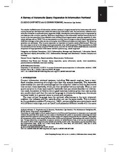
Figure 2. Sample of 20 query images used in the ground truth evaluation. For all query images see [12].

visual-words model. These quantized visual features are then used to index the images for the search engine. Search Engine. Our search engine uses the vector-space model of information-retrieval. The query and each document in the corpus is represented as a sparse vector of term (visual word) occurrences and search then proceeds by calculating the similarity between the query vector and each document vector. We use the standard tf-idf weighting scheme [3], which down-weights the contribution that commonly occurring, and therefore less discriminative, words make to the relevance score. For computational speed, the engine stores word occurrences in an index, which maps individual words to the documents in which they occur. For sparse queries, this can result in a substantial speedup over examining every document vector, as only documents which contain common (to the query) words need to be examined. The scores for each document are accumulated so that they are identical to explicitly computing the similarity. With large corpora of images, memory usage becomes a major concern. To help ameliorate this problem, the inverted file is stored in a space-efficient binary-packed structure. Additionally, when main memory is exhausted, the engine can be switched to use an inverted file flattened to disk, which caches the data for the most frequently requested words.

3. Spatial Verification The output from performing a query on the inverted file described previously is a ranked list of images for a significant section of the corpus. Until now, we have considered the features in each image as a visual bag-of-words and have ignored their spatial configurations. It is vital for query-expansion that we do not expand using false positives or use features which occur in the result image, but not on

the object of interest. To achieve this, we use a fast, robust, hypothesize and verify procedure to estimate an affine homography between a query region and target image. Each interest point has an affine invariant semi-local region associated with it and we use this extra information to hypothesize transformations using single correspondences. This makes our procedure both fast (the number of hypotheses to test is simply the number of putative correspondences) and deterministic (we examine every possible hypothesis). A RANSAC-like scoring mechanism is used to select the hypothesis with the greatest number of inliers. Each single correspondence hypothesizes a three degree of freedom (dof) transformation (isotropic scale & translation). For a typical query of 1000 features, with a discriminative vocabulary, the number of correspondences and hence hypotheses to test will be of the order of a few thousand. The number of inliers to this transformation is found using a symmetric transfer error [7] coupled with a scale threshold which prevents mis-sized regions from scoring as inliers. Each hypothesis is stored in a priority queue, keyed by the number of inliers. For the top 10 hypotheses found, we iteratively use a least-squares re-estimation method on the initially found inliers to generate a full 6 dof affine transformation, returning the best hypothesis as the one with the most inliers after re-estimation [5]. Empirically, we find that results with more than 20 inliers reliably contain the object being sought for. We call such results spatially verified. The spatial verification is applied up to a maximum of the top 1000 results returned from the search engine. At each result, a decision is made about whether to proceed with the verification further down the ranked list based on how recently a verified image has been seen. If no verified result has been seen in the last 20 ranked images, then we stop, returning the verified images seen so far. Empirically, we find that increasing this threshold further does not significantly increase the number of positively verified results. This prevents us from needlessly verifying images for results where all the true positive images have already been seen, or from prematurely bailing out of verification when there are more true positives waiting to be found. The output is a list of images ranked in non-increasing order of the number of inliers. The threshold of 20 inliers is used to produce a list of verified results and their associated transformations. This list of known good results is essential for the query expansion.

4. Generative Model In this section, we describe several methods for computing latent object models. These are based on generative models of the features and their configuration, with different levels of complexity. We account for quantization and detection noise, and the effect of different image resolutions.

Each method starts by evaluating the original query Q0 composed of all the visual words which fall inside the query region. A latent model is then constructed from the verified images returned from Q0 , and a new query Q1 , or several new queries, issued. This immediately raises two issues: (i) how far should this sequence extend – should a new latent model be built from the returns of Q1 and another query issued, etc? (ii) how should the ranked lists returned from Q0 , Q1 , . . . be combined? We explore both these questions. Note that the bag-of-visual-word result set from Q1 must be verified against Q1 – for example Q0 cannot be used for verification since we are aiming to obtain images that were not verified against Q0 .

4.1. Methods The methods can be divided into those that issue a single new query and those that issue multiple queries. In the latter case it is necessary to combine the returned ranked lists for each query. Query expansion baseline. This method is a straight forward na¨ıve application of query expansion as is used in textretrieval. We take the top m = 5 results from the original query (without spatial verification), average the termfrequency vectors computed from the entire result image and requery once. The results of Q1 are appended to those of Q0 (the top 5). Transitive closure expansion. A priority queue of verified images is keyed by the number of inliers. Then, an image is taken from the top of the queue and the region corresponding to the original query region is used to issue a new query. Verified results of the expanded query that have not been inserted to the queue before are inserted (again in the order of the number of inliers). The procedure repeats until the queue is empty. The images in the final result are in the same order in which they entered the queue. Average query expansion. A new query is constructed by averaging verified results of the original query. First, the top m < 50 verified results returned by the search engine are selected. A new query Qavg is then formed by taking the average of the original query Q0 and the m results ! m X 1 davg = d0 + di , m+1 i=1 where d0 is the normalized tf vector of the query region, and di is the normalized tf vector of the i-th result. For this average, we take the union of features of the original query, combined with regions back-projected into the query region by Hi – the estimated transformation. This is the simplest form of latent model since no account is taken of the stability of the features or the resolution of the images. Again we requery once, and the results of Qavg are appended to those (top m) of Q0 .

Recursive average query expansion. This method improves on the average query expansion method, by recursively generating queries Qi from all spatially verified results returned so far. The method stops once more than 30 verified images have been found, or after no new images have been positively verified. Multiple image resolution expansion. The generative model in this case also takes account of the probability of observing a feature given an image of an object and its resolution. Features covering a small area of the object are seen only in close-up images or images with high resolution. Similarly, features covering the whole object are not seen on detailed views. The latent image is constructed as before by back projecting verified regions of Q0 using the Hi transformations. The number of pixels of the projected region defines the resolution of each result image. An image with median resolution is chosen as a resolution reference image and a relative change of the resolution (with respect to the resolution reference image) is computed for each result image. The resolution bands are given by the relative resolution change as (0, 4/5), (2/3, 3/2), and (5/4, ∞). We construct an average query for each of the three different resolution bands, using only images that have resolution within that scale band. The queries are executed independently and the results are merged. Verified images from Q0 are returned first. Results from expanded queries follow in order of the number of inliers (the maximum is taken if an image is retrieved in more than one resolution band).

5. Experiments To evaluate our system, we use the Oxford dataset available from [2]. This is a relatively small set of 5K images with an extensive associated ground truth. We also use two additional unlabeled datasets, Flickr1 and Flickr2, which are assumed not to contain images of the ground truth landmarks. These additional datasets are used as “distractors” for the system and provide an important test for the scalability of our method. These three datasets are described below and compared in table 1. The set of images downloaded from two or more of Flickr’s tags will not in general be disjoint, so we remove exact duplicate images from all our datasets. The Oxford dataset. This dataset [2] was crawled from Flickr using queries for famous Oxford landmarks, such as “Oxford Christ Church” and “Oxford Radcliffe Camera”. It consists of 5,062 high resolution (1024 × 768) images. Ground truth labelling is provided for 11 landmarks with four possible labels as follows: (1) Good – a nice, clear picture of the object/building. (2) OK – more than 25% of the object is clearly visible. (3) Bad – the object is not present. (4) Junk – less than 25% of the object is visible, or there is a very high level of occlusion or distortion. For each

Number of images 5,062 99,782 1,040,801 1,145,645

Number of features 16,334,970 277,770,833 1,186,469,709 1,480,575,512

All Souls

Dataset Oxford Flickr1 Flickr2 Total

Table 1. The number of descriptors for each dataset.

To evaluate performance we use Average Precision (AP) computed as the area under the precision-recall curve. Precision is the number of retrieved positive images relative to the total number of images retrieved. Recall is the number of retrieved positive images relative to the total number of positives in the corpus. An ideal precision-recall curve has precision 1 over all recall levels, which corresponds to an Average Precision of 1. Note, a precision-recall curve does not have to be monotonically decreasing. To illustrate this, say there are 3 positives out of the first 4 retrieved, which corresponds to precision 3/4 = 0.75. Then, if the next image is positive the precision increases to 4/5 = 0.8. We compute an Average Precision score for each of the 5 queries for a landmark, and then average these to obtain a Mean Average Precision (MAP) for the landmark. For some experiments, in addition to the MAP, we also display precision-recall curves which can sometimes better illustrate the success of our system in improving recall. In the evaluation the “Good” and “Ok” images are treated as positives, “Bad” images as negative and “Junk” images as “don’t care”. The “don’t care” images are handled as if they were not present in the corpus, so that if our system returns them, the score is not affected. We evaluate our system on two databases – D1 composed of Oxford + Flickr1 datasets (104,844 images) and D2 Oxford + Flickr1 + Flickr2 datasets (1,040,801 images). The effect of the size of the database on the performance is discussed in section 5.4.

0.6

0.6

0.4

0.4

0.2

0.2

Ashmolean Hertford

0.4

0.6

0.8

1

0 0 1

0.8

0.6

0.6

0.4

0.4

0.2

0.2

0.2

0.4

0.6

0.8

1

0 0 1

0.8

0.8

0.6

0.6

0.4

0.4

0.2

0.2

0 0 1

Keble

0.2

0.8

0 0 1

0.2

0.4

0.6

0.8

1

0 0 1

0.8

0.8

0.6

0.6

0.4

0.4

0.2

0.2

0 0 1

Magdalen

5.1. Evaluation procedure

1

0.8

0 0 1

0.2

0.4

0.6

0.8

1

0 0 1

0.8

0.8

0.6

0.6

0.4

0.4

0.2

0.2

0 0 1

Radcliffe camera

landmark five standard queries are defined for evaluation. A sample of 20 query images is shown in figure 2, for the rest see [2]. Flickr1 dataset. This dataset was crawled from Flickr’s 145 most popular tags and consists of 99,782 high resolution images. Our search engine can query the combined datasets of Oxford and Flickr, consisting of 104,844 images, in around 0.1s for a typical query and the index consumes 1GB of main memory. Flickr2 dataset. This dataset consists of 1,040,801 medium resolution (500 × 333) downloaded from Flickr’s 450 most popular tags. The index for the combined Oxford, Flickr1 and Flickr2 corpus is 4.3GB, so we use an offline version of the index which does not have to sit in main memory. Querying this corpus from disk takes around 15s – 35s for a typical query.

1

0.8

0.2

0.4

0.6

0.8

1

0 0 1

0.8

0.8

0.6

0.6

0.4

0.4

0.2

0.2

0 0

0.2

0.4

0.6

0.8

1

0 0

0.2

0.4

0.6

0.8

1

0.2

0.4

0.6

0.8

1

0.2

0.4

0.6

0.8

1

0.2

0.4

0.6

0.8

1

0.2

0.4

0.6

0.8

1

0.2

0.4

0.6

0.8

1

Figure 3. Precision recall curves before (left) and after (right) query expansion on experiment D1. These results are for resolution expansion, our best method. In each case the five curves correspond to the five queries for that landmark.

5.2. Retrieval performance In this section, we discuss some quantitative results of our method evaluated against the ground truth gathered from the Oxford dataset. Table 2 summarizes the results of using our different query expansion methods, measuring their relative performance in terms of the MAP score. From the table, we can

Ground truth OK Junk All Souls 78 111 Ashmolean 25 31 Balliol 12 18 Bodleian 24 30 Christ Church 78 133 Cornmarket 9 13 Hertford 24 31 Keble 7 11 Magdalen 54 103 Pitt Rivers 7 9 Radcliffe Cam. 221 348 Total 539 838

ori 41.9 53.8 50.4 42.3 53.7 54.1 69.8 79.3 9.5 100 50.5 55.0

Oxford + Flickr1 dataset qeb trc avg rec 49.7 85.0 76.1 85.9 35.4 51.4 66.4 74.6 52.4 44.2 63.9 74.5 47.4 49.3 57.6 48.6 36.3 56.2 63.1 63.3 60.4 58.2 74.7 74.9 74.4 77.4 89.9 90.3 59.6 64.1 90.2 100 6.9 25.2 28.3 41.5 100 100 100 100 59.7 88.0 71.3 73.4 52.9 63.5 71.1 75.2

sca 94.1 75.7 71.2 53.3 63.1 83.1 97.9 97.2 33.2 100 91.9 78.2

Oxford + Flickr1 + Flickr2 dataset ori qeb trc avg rec sca 32.8 36.9 80.5 66.3 73.9 84.9 41.8 25.9 45.4 57.6 68.2 65.5 40.1 39.4 39.6 55.5 67.6 60.0 32.3 36.9 43.5 46.8 43.8 44.9 52.6 18.9 55.2 61.0 57.4 57.7 42.2 53.4 56.0 65.2 68.1 74.9 64.7 70.7 75.8 87.7 87.7 94.9 55.0 15.6 57.3 67.4 65.8 65.0 5.4 0.2 16.9 15.7 31.3 26.1 100 90.2 100 100 100 100 44.2 56.8 86.8 70.5 72.5 91.3 46.5 40.5 59.7 63.1 67.0 69.6

Table 2. Summary of ground truth, and the relative performance of the different expansion methods. The methods are as follows: ori – original query, qeb – query expansion baseline, trc - transitive closure, avg – average query expansion, rec – recursive average query expansion, sca – resolution expansion. The shade of each cell shows relative performance to the worst (dark) and the best (white) result for a particular query (row).

original query

6

4

2

0

0.2

0.4

0.6

0.8

1

0.2

0.4

0.6

0.8

1

resolution expansion

6

4

2

0

AP Figure 4. Histograms of the average precision for all 55 queries in experiment D2. Note, that the query expansion moves the mass of the histogram towards the right-hand side, i.e. towards total recall.

Figure 5. Some false positive images for Magdalen Tower query. The tower shown is actually part of Merton College chapel.

see that all proposed query expansion (with the exception of the query expansion baseline) methods perform much better than the original bag-of-visual-words method, showing a gain in the MAP from 55.0% to 78.2% on D1 and from 46.5% to 69.6% on D2 with the best method. Figure 3 shows selected precision recall curves for the

plain bag-of-words method on the left, with the curves from the resolution-based query expansion shown on the right. In almost all cases, the precision recall curve hugs to the right of the graph much more after the query expansion, demonstrating the method’s power in dramatically improving the recall of a query. Additionally, in the original bag-of-words query, each individual query for the landmarks shows considerable variance in the precision-recall plots, whereas after query expansion has been applied, in most cases, this variance has been reduced, improving all the component queries to a similar level of retrieval performance. The plot for Magdalen in figure 3, shows failure in achieving total recall. If the initial results returned from the bag-of-words method are too bad, so that there are no verified images with which to query expand, our method is unable to improve the performance. This occurs for two of the Magdalen queries. Note, that since we are measuring the MAP over all queries, the average result in table 2 is lowered by such non-expandable queries. To eliminate the averaging effect we study each query independently. Figure 4 compares two histograms of AP for each of the 55 queries on experiment D2. The top histogram displays results of the original query and the bottom results of the best query expansion method. The plot clearly shows the significant improvement brought by the query expansion. The performance of the system is hurt by incorrectly verified retrievals. No verification method is perfect, especially when one has to deal with partial occlusions. Some of the false positives are indeed difficult to distinguish, even for a human, as demonstrated in figure 5. Figure 6 shows some example images returned by our method, which were not found in the original bag-of-words query. After query expansion, we get many more examples

Figure 6. Demonstrating the performance of the method on a number of different queries. The image to the left shows the original query image. The four images in the middle show the first four results returned by the original query before query expansion. The images to the right show true positive images returned after query expansion which were not found from the bag-of-words method.

of the object, some of which would be extremely challenging to the traditional method, with, in some cases, very high levels of occlusion or large scale changes.

5.3. Method comparison We now compare our different query expansion methods, referring to table 2 for the relative performances. Query expansion baseline (qeb). This method does worse than not using query expansion at all, as expected. Blindly choosing the top m documents for expansion does not take into account whether or not any of the top m are correct, so the method suffers from serious drift. We can see this by noting that queries which return lots of true positives from the initial query, such as Radcliffe Camera and Hertford perform much better than those with fewer initial true

positives, such as Ashmolean and Keble. Transitive closure (trc). The method uses a single image to query with each time. Since both the feature detection and vocabulary generation are noisy processes, transitive closure has lower performance than methods constructing latent image representation from several images. This method the slowest since it generates by far the highest number of query reissues. Average query expansion (avg). This method performs significantly better than just using the results from the standard bag-of-words methods, scoring on average 71.1% as opposed to 55.0% in the case of D1. Additionally, the method improves the results for every query in our scoring. This method performs so much better mainly because the spatial verification allows us to exclude false positives from

results to the original query, preventing the “drift” which ruined the baseline method. Recursive average query expansion (rec). This method improves on the avg method, by recursively generating and querying the system with spatially verified results. By querying recursively, we can more thoroughly explore the space of object features, giving us instances of the object whose visual appearance can differ greatly from the original query. Resolution expansion (sca). The resolution expansion method performs the best on our data. By grouping results based on the resolution of the object of interest, we query expand using only features which reliably fire on the object at a particular resolution. This prevents us from including features which fire at different scales, which can raise the chance of a false positive image being verified. This method gets an MAP score of 78.2% on D1 and 69.6% on D2 and most of the 55 queries exhibit near total recall, see figure 4. The percentage is brought down by a few queries, which due to the initial bad performance of the bag-of-words method are unable to be successfully expanded. Such queries lie on the left-hand side of the lower histogram in figure 4. Also, note that the merging strategy does not rank all images in the database. This can be observed on the precision recall (figure 3) where the curve does not reach the right side of the plot.

5.4. Dataset comparison D1 vs. D2 The average precision measure is designed to capture quality of retrieval with strong emphasis on the top ranked results. Note, that additional negative images can only decrease (or leave unchanged) the average precision measure. In the best case, if all of the additional negative images were correctly classified, they could be appended at the tail of the results which would leave average precision unchanged. However, correct classification of all images rarely happens. Our experiments show varying drop of performance after increasing the size of the database (negative images) 10 times. The decrease in performance (relative and absolute) is lower for query expansion methods than for the original method.

6. Discussion Given the set of retrieved images, which often cover a variety of viewpoints, we now have the potential to construct much richer latent feature models of the query region. Much previous work – Ferrari et al. [6], Lowe [8], Rothganger et al. [15] – has explored combining features from multiple views and this can now be harnessed for latent model construction. It is also possible to move from features to surfaces – where the latent model would consist of a textured 3D surface reconstruction, which can be built

using standard methods [7, 13]. We view image-retrieval systems such as Video Google as one extreme, and the “Photo Tourism” system [19] as another, of examples drawn from a spectrum of possible image-based object retrieval techniques. The common feature unifying this family of methods is that they construct a “latent model” of the query object with the aid of the image corpus, and return to the user some representation of that latent model. The work of this paper defines another point on the spectrum. Acknowledgements We are grateful for support from an EPSRC Platform grant, the Royal Academy of Engineering, EU project C LASS and Microsoft.

References [1] http://www.flickr.com/. [2] http://www.robots.ox.ac.uk/∼vgg/data/oxbuildings/. [3] R. Baeza-Yates and B. Ribeiro-Neto. Modern Information Retrieval. ACM Press, ISBN: 020139829, 1999. [4] C. Buckley, G. Salton, J. Allan, and A. Singhal. Automatic query expansion using smart. In TREC-3 Proc., 1995. [5] O. Chum, J. Matas, and J. Kittler. Locally optimized RANSAC. In DAGM, 2003. [6] V. Ferrari, T. Tuytelaars, and L. Van Gool. Simultaneous object recognition and segmentation by image exploration. In Proc. ECCV, 2004. [7] R. I. Hartley and A. Zisserman. Multiple View Geometry in Computer Vision. Cambridge University Press, ISBN: 0521540518, second edition, 2004. [8] D. Lowe. Local feature view clustering for 3D object recognition. In Proc. CVPR, pages 682–688. Springer, 2001. [9] D. Lowe. Distinctive image features from scale-invariant keypoints. IJCV, 60(2):91–110, 2004. [10] K. Mikolajczyk and C. Schmid. Scale & affine invariant interest point detectors. IJCV, 1(60):63–86, 2004. [11] D. Nister and H. Stewenius. Scalable recognition with a vocabulary tree. In Proc. CVPR, 2006. [12] J. Philbin, O. Chum, M. Isard, J. Sivic, and A. Zisserman. Object retrieval with large vocabularies and fast spatial matching. In Proc. CVPR, 2007. [13] M. Pollefeys, L. Van Gool, and M. Proesmans. Euclidean 3D reconstruction from image sequences with variable focal lengths. In Proc. ECCV, LNCS 1064/1065. Springer-Verlag, 1996. [14] T. Quack, V. Ferrari, and L. Van Gool. Video mining with frequent itemset configurations. In Proc. CIVR, 2006. [15] F. Rothganger, S. Lazebnik, C. Schmid, and J. Ponce. 3D object modeling and recognition using affine-invariant patches and multiview spatial constraints. In Proc. CVPR, 2003. [16] G. Salton and C. Buckley. Improving retrieval performance by relevance feedback. Journal of the American Society for Information Science, 41(4):288–297, 1999. [17] C. Schmid and R. Mohr. Combining greyvalue invariants with local constraints for object recognition. In Proc. CVPR, pages 872–877, 1996. [18] J. Sivic and A. Zisserman. Video Google: A text retrieval approach to object matching in videos. In Proc. ICCV, Oct 2003. [19] N. Snavely, S. Seitz, and R. Szeliski. Photo tourism: exploring photo collections in 3d. In Proc. ACM SIGGRAPH, pages 835–846, 2006. [20] D. Tell and S. Carlsson. Combining appearance and topology for wide baseline matching. In Proc. ECCV, LNCS 2350, pages 68–81. Springer-Verlag, May 2002.