Feb 23, 2017 - atively little success in high-throughput identification of the intercellular ... dom forest and other classical machine learning approaches that are ...
Toward Streaming Synapse Detection with Compositional ConvNets Shibani Santurkar David Budden Alexander Matveev Heather Berlin Hayk Saribekyan Yaron Meirovitch Nir Shavit Massachusetts Institute of Technology
arXiv:1702.07386v1 [cs.CV] 23 Feb 2017
{shibani,budden,amatveev,hberlin,hayks,yaronm,shanir}@mit.edu
Abstract
largely replaced by high-throughput pipelines responsible for automated segmentation and morphological reconstruction of neurons from nanometer-scale electron microscopy (EM) [8, 9, 10, 11, 12]. Automation is critical for any largescale investigation of neuron organization, as even a humble 1 mm3 volume of tissue contains many petabytes of EM data at the necessary resolution. Of course, reconstructing 3-dimensional models of neuron “skeletons” is only a partial solution to the larger goal of constructing neuron connectivity maps. Individual neurons are very densely packed but their connectivity is comparatively sparse, thus deriving connectivity is more complex than simply identifying the cell membranes of adjacent neurons. In recent years, several frameworks have been published that segment neurons with near-human accuracy [8, 9, 10, 11, 12]. However, there has been substantially less success in identifying synapses – the junctions whereby neurons connect and communicate. In the context of a neural connectivity graph, this is equivalent to identifying nodes but ignoring the edges between them. Synapses are inherently compositional, identifiable in EM by a darkened cleft between adjacent neurons flanked by an asymmetric density of vesicles (neurotransmittercarrying organelles). Accordingly, most previous approaches to synapse detection have used classifiers (typically random forests) with hand-crafted features to leverage this prior knowledge. Early examples include the work of Kreshuk et al., which captured voxel geometry and texture [13]; and Becker et al., who extended this work to capture 3-dimensional contextual cues [14]. Although these approaches worked well on the datasets for which they were trained, they failed to generalize beyond the specific contrast and anisotropy (4 × 4 × 45 nm) of that dataset [15].
Connectomics is an emerging field in neuroscience that aims to reconstruct the 3−dimensional morphology of neurons from electron microscopy (EM) images. Recent studies have successfully demonstrated the use of convolutional neural networks (ConvNets) for segmenting cell membranes to individuate neurons. However, there has been comparatively little success in high-throughput identification of the intercellular synaptic connections required for deriving connectivity graphs. In this study, we take a compositional approach to segmenting synapses, modeling them explicitly as an intercellular cleft co-located with an asymmetric vesicle density along a cell membrane. Instead of requiring a deep network to learn all natural combinations of this compositionality, we train lighter networks to model the simpler marginal distributions of membranes, clefts and vesicles from just 100 electron microscopy samples. These feature maps are then combined with simple rules-based heuristics derived from prior biological knowledge. Our approach to synapse detection is both more accurate than previous state-of-the-art (7% higher recall and 5% higher F1-score) and yields a 20-fold speed-up compared to the previous fastest implementations. We demonstrate by reconstructing the first complete, directed connectome from the largest available anisotropic microscopy dataset (245 GB) of mouse somatosensory cortex (S1) in just 9.7 hours on a single shared-memory CPU system. We believe that this work marks an important step toward the goal of a microscope-pace streaming connectomics pipeline.
1. Introduction Rigorous studies of neural circuits in mammals could uncover motifs underlying information processing and neuropathies at the core of disease [1, 2, 3, 4]. Traditionally these studies involved the painstaking manual tracing of individual neurons through microscopy data [5, 6, 7]. In the modern connectomics field, this manual effort has been
In recent years, deep convolutional networks (ConvNets) have become a de facto standard for image classification [16] and semantic segmentation [17]. When provided with sufficient training data, ConvNets typically outperform random forest and other classical machine learning approaches that are dependent on hand-crafted features. It is per1
(a)
Electron Microscopy
Marginal ConvNets
Composition
neuron membrane
intercellular cleft
∫
synaptic vesicles
(b)
Output
vesicles
synapses
Figure 1: (a) Workflow summary of our synapse detection. Raw electron microscopy (EM) data is streamed into lightweight parallel ConvNets, each trained to recognize a specific feature—one of neuron membranes, intercellular clefts or synaptic vesicles. (b) The output probability maps of each of these marginal features are then composed using prior biological knowledge to identify synapses (red). The asymmetric density of vesicles (blue) can also be leveraged to infer directionality of connectivity graphs.
haps then unsurprising that the most accurate framework for synapse detection in previous literature is a ConvNet (Vesicle-CNN) by Roncal et al., which is trained to segment synapses directly from EM data without any prior knowledge of clefts, vesicles and their compositionality [18]. The authors also published a much faster yet less accurate random forest classifier (Vesicle-RF), which outperforms previous approaches by explicitly modeling properties of synaptic connections. The major issue with ConvNets (including VesicleCNN) is that they are prohibitively slow. Biologically meaningful volumes of neural tissue take months-to-years to image, thus a critical step toward the goals of connectomics is developing a computational pipeline that can process streaming data at microscope pace [12, 19]. The authors of Vesicle-CNN reported a processing time of 400 hours per GB of EM [18], i.e., several orders-ofmagnitude slower than the TB/hr pace of modern multibeam electron microscopes. Their lightweight Vesicle-RF was both substantially faster yet less accurate, making it impractical for connectomics where reliable synapse identi-
fication is needed for detecting enrichment of neural motifs. In this study we present a new synapse detection framework that attempts to distill the advantages of both accurate ConvNets and faster knowledge-driven techniques. Rather than training a deep ConvNet to segment synapses directly from EM samples, we train much lighter networks to learn the marginal distributions of neuron membranes, intercellular clefts and synaptic vesicles. These features are then explicitly composed with simple rules that follow directly from prior biological knowledge. The resulting system (see Figure 1) is both faster and more accurate compared to state-of-the art—11000× speed-up and +3% F1-score over the accurate Vesicle-CNN and 20× speed-up and +5% F1score over the faster yet less accurate Vesicle-RF. We apply our system to reconstruct the first complete, directed connectome from the largest available anisotropic EM dataset of mouse somatosensory cortex (S1 [5]). This 245 GB reconstruction took just 9.7 hours on one multicore CPU, end-to-end from EM to connectivity graphs. Compare this to the previous largest 56 GB reconstruction, which needed 3 weeks to segment neuron membranes (on a farm of 27 Titan X GPUs) and a further 39 hours to identify synapses using Vesicle-RF on a 100−core CPU cluster [20].
2. Compositional ConvNets In this section we describe our synapse detection system, which is both faster and more accurate than state-of-the-art and able to be run on a single multicore CPU server. This system is comprised of two main parts: (1) a bank of three lightweight ConvNets that can be deployed in parallel to segment membranes, clefts and synaptic vesicles; and (2) a rules-based module that integrates these three feature maps to identify synapses. The intuition behind this approach is to constrain the space in which our ConvNets are optimized by leveraging prior biological knowledge on synapse compositionality, i.e. the network simply has less to learn. This both avoids the computational burden associated with the traditional “deeper is better” ConvNet paradigm while empirically improving synapse detection accuracy across the 245 GB S1 dataset.
2.1. Marginal Segmentation Deep ConvNets of small kernels have become a de facto standard for image classification tasks, largely motivated by the success of AlexNet [16] and progressively deeper networks [21, 22, 23] in the annual ImageNet classification challenge [24]. More recently ConvNets have been used to solve semantic segmentation tasks [17], which require assigning a class label or probability to each pixel of the output feature map. There have been several successful examples of ConvNets being applied successfully to segmentation of neuron membranes from EM data [8, 9, 10, 11, 25].
(a)
input
FConv
4x4 stride 1 2
FCPool
maxout
2x2 stride 2
(b) 4 matric es
Conv Pool
16 mat
64 mat
...
...
rices
Conv Pool
...
rices
Conv Pool
membra
nes
...
(S1)
...
6 nm EM
...
(a)
Figure 2: Lightweight ConvNet architecture used to detect synapses, vesicles and membranes. (a) Each ConvPool layer consists of alternating convolution/maxpool layers combined with a maxout function. (b) The full network comprises three consecutive ConvPool layers followed by a binary softmax. Our implementation is fully convolutional using the maxpooling fragments technique [26, 27].
Figure 3: Example of synapses and vesicles detected by our system, superimposed on raw electron microscopy samples. Examples show correctly identified ground truth synapses (red), missed ground truth synapses (blue), correct predictions (green), faulty predictions (yellow), and vesicle clusters (cyan).
2.1.1 In the context of reconstructing connectivity graphs, this is akin to defining the set of nodes but not edges. In our system, we deploy lightweight ConvNets to learn the marginal distributions of (a) neuron membranes, (b) intercellular clefts and (c) synaptic vesicles. Our approach to segmenting neuron membranes is essentially equivalent to prior work in [11]. The network is presented with 1024 × 1024 EM images at 6 nm resolution and associated ground-truth segmentations, and learns to produce an output segmentation in the form of a spatial membrane probability map (normalized to the integer range [0, 255]). Synaptic clefts are treated largely the same, focusing on the darkened regions between a subset of adjacent cellular membranes. Our approach to vesicle detection is more unique. Vesicles are organelles that store the various chemicals required for neurotransmission, and are located at the pre-synaptic partner of neuron connections. Automatic detection of vesicles has previously been considered a difficult task [13] and has thus not been extensively studied. To our knowledge Vesicle-RF was the first system to attempt to identify individual vesicles (using a hand-crafted match filter) to assist with synapse identification [18]. Unlike their approach, we train a ConvNet to segment significant clusters of spatially co-located vesicles as a single feature (cyan in Figure 3). In addition to allowing us to reconstruct directed connectivity by considering vesicle density in the pre- vs. post-synaptic partners, there is also a well-established correlation between this density and the strength of synaptic connections [7] (akin to weights in an artificial neural net).
(b)
ConvNet Implementation
Each of our three marginal ConvNets adopts the same lightweight architecture (herein MaxoutNet, Figure 2) that comprises of consecutive “ConvPool” modules. Each module consists of two parallel branches aggregated with a Maxout function [11], where each branch is a convolution operation (kernel size k = 4 × 4, 32 channels) followed by a 2 × 2 maxpool of stride 2. The full network consists of three consecutive ConvPool modules followed by a final 6 × 6 kernel to output the segmented feature map. There are a number of compounding factors that allow our system to execute orders-of-substantially faster than previous state-of-the-art. First is the lightweight nature of the MaxoutNet architecture, which contains orders-ofmagnitude fewer parameters than previous popular connectomics ConvNets (i.e., ∼ 105 compared to UNet’s ∼ 107 [9]). Second is our minimally fully-convolutional implementation, inspired by fast algorithms of max-pooling fragments [26, 27]. Compared with naive patch-based methods of semantic segmentation (i.e., where the full convolutional field-of-view is reprocessed for every output pixel) this method leads to a 200−fold reduction in redundant computations. Finally is our multicore CPU-optimized implementation, which makes liberal use of SIMD instructions [28] and Cilk-based job scheduling [29] to yield 70−80% singlecore utilization and 85% multi-core scalability across our 8−core Haswell processor. The aggregate impact of these optimizations is an 11, 000−fold speed-up with respect to Vesicle-CNN [18]. It is worth noting that Vesicle-CNN reports to be based on the N3 ConvNet architecture [10] but uses stride-1 instead of stride-2 pooling, which is largely responsible for the inflation of their network size.
Figure 4: Example of neuron-level segmentation for a small sub-volume of the S1 dataset. This is reconstruction is achieved by (1) generating membrane segmentations with our lightweight marginal ConvNet, (2) producing an oversegmentation by applying the Watershed algorithm, and (3) merging adjacent segments with the Neuroproof package [30]. This segmentation is composed with intercellular clefts and synaptic vesicles to identify synapses.
2.2. Synapse Composition In recent years the ConvNet paradigm has been one of “deeper is better”, with more complex problems being solved by increasing network depth and data volume [16, 21, 22]. This is also the Vesicle-CNN approach to synapse detection [18], which segments synapses directly from EM without explicitly capturing any prior biological knowledge. Although this approach certainly has merit (as reflected in state-of-the-art performance on ImageNet and other image processing benchmarks [31]) it does not extend well to problems where real-time performance is a hard constraint. Connectomics is one such problem [19]. If a biologically meaningful volume of neural tissue already takes months-to-years to image with modern multi-beam electron microscopy, we certainly do not wish to exacerbate this problem with post-processing that is orders-of-magnitude slower. Further, producing ground-truth annotation for EM data is done manually and is highly time-consuming, taking even expert neuro-scientists hundreds of hours. As a result, the volume of training data available is extremely limited and there is need to design algorithms which are resilient to this. This motivates our choice of shallow networks, to avoid overfitting associated with deep networks in data-constrained problems.
In our system, we leverage the explicit compositionality of synapses to greatly reduce the search space within which our ConvNets are optimized (i.e. learning marginal versus joint distributions over features). This reduction in search space is explicitly captured by a lightweight network architecture, and thus able to be leveraged for substantial speedup in synapse segmentation. To accomplish this, we take motivation from the concept of compositional hierarchies, wherein low-level features are explicitly composed to perform tasks such as object recognition [32, 33, 34, 35] and scene parsing [36, 37]. It has been shown that in various recognition tasks, the use of hierarchies is more informative than non-hierarchical representations [38] and yields improved performance and generalizability, especially in the presence of occlusion or clutter [39, 40]. Such compositionality is also believed to be an intrinsic mechanism for object recognition in the visual cortex [41, 42]. A key shortcoming of traditional compositional models is the difficulty of hand-crafting feature hierarchies for the expansive domain of natural images, or building suitable models to learn these features in an unsupervised fashion. This is one of the key motivators behind recent deep learning trends, although ConvNets are likewise criticized for their absence of compositionality [43] and feature intelligibility [44]. Instead, our approach distils the advantages of both domains. Rather than capturing low-level features using Gabor filters or SIFT features, we take motivation from the work of Ullman et al. in natural image classification [35] and explicitly compose pictorial features. Unlike previous work, our pictorial features are not crops of the raw EM but instead taken from the ConvNetsegmented features maps of membranes, clefts and vesicles. Here, learning feature (membranes, clefts and vesicles) segmentation using ConvNets is easier than learning synapses because of two primary reasons—(1) relative simplicity of features as compared to synapses (2) availability of significantly more ground truth for features (for e.g., the number of membrane pixels in an annotated EM stack is a few orders of magnitude larger than the number of synaptic pixels due to the sparsity of neural connections). Neuron membranes predicted by the ConvNet are further processed to segment individual neurons in the traditional manner [20]. Specifically, we generate an oversegmentation of neurons using the popular Watershed algorithm. These segments are then agglomerated using the NeuroProof package by Parag et al., which applies a pretrained random forest classifier to determine which adjacent segments require merging [30]. In both cases we use custom implementations optimized for multicore CPU scalability [45, 46]. An example output of this process is presented in Figure 4 for a small sub-volume of the S1 dataset. Neuron segmentations are then composed with cleft and vesicle segmentations to filter putative synapse candidates. This in-
post-synaptic neurons with an inter-cellular synapse) without need for further processing or manual intervention.
3. System Evaluation
(a)
(b)
(c)
Figure 5: Automatic reconstruction of synapses from AC3 region of mouse S1. The axon/pre-synaptic neuron (green) and the dendrite/post-synaptic neuron (blue) interface via the synaptic cleft (red). The compositional nature of our system greatly simplifies the extraction of directionality. volves applying the following rules:
We chose to evaluate our system performance, both in terms of reconstruction accuracy and execution time, on the largest available connectomics dataset. Specifically, the S1 dataset by Kasthuri et al. is an anisotropic EM volume of mouse somatosensory cortex imaged at 3 × 3 × 29 nm resolution, containing an estimated 0.5 − 1 synapses/um3 [47]. This dataset is color-corrected and down-sampled to 6 × 6 × 29 nm prior to processing. We compare our performance against the two state-ofthe-art systems for synapse detection by Roncal et al. – the highly accurate ConvNet-based Vesicle-CNN and the faster but less accurate, random forest-based Vesicle-RF [18]. We select two independent 1024 × 1024 × 100 volumes of S1 for testing (AC3) and training/validation (AC4). Groundtruth annotations for these sub-volumes have been provided by expert neuroscientists [48].
3.1. Evaluation Metrics 1. Restrict candidates to membrane regions and discard intra-cellular predictions 2. Constrain predictions to be within a certain maximum distance to vesicles. We are interested in finding active synapses typically marked by the presence of vesicles 3. Threshold (binary) synapse probabilities with an empirically tuned parameter. 4. Break large synapse predictions that cover many true and false synapses. This ensures each connected synapse candidate lies between a unique pair of neurons. This is important to find pre- and post-synaptic neurons for a synapse. 5. Connected component analysis and checks on minimum 2D/3D size and slice persistence (similar to Vesicle-RF). 6. Reject candidates that do not contain vesicles in one of the two neuron segments they connect. This additional check ensures that all the final synapse candidates are active and contain vesicles in close proximity, in one of the two adjoining segments. A few examples of synapses (red) detected using our system are presented in Figure 5. The axon (pre-synaptic partner, green) and dendrite (post-synaptic partner, blue) are trivially identified from asymmetric vesicle density in our compositional model. Extracting directionality from Vesicle-RF/CNN or similar approaches would require additional layers of post-processing. As a result, our approach is the first to enable scalable inference of the the wiring diagram (defined as a graph connecting pairs of pre- and
Various metrics of pixel-level accuracy have been presented for various image segmentation challenges [49]. However, in the connectomics scenario we are less interested in the pixel-level fidelity of synapse segmentation (i.e. the metric used for training and evaluating ConvNets) as long as we are correctly identifying the existence of a synaptic connection. This is convenient as it allows us to deploy far lighter networks without reducing the accuracy of the downstream connectivity graph. For our benchmarking we consider the following metrics prescribed by IARPA for the MICrONs project [50] and used widely within the connectomics community [18, 20]: 1. Synapse Detection Accuracy: Precision, recall and F1-score (harmonic mean of precision of recall) of identified synapses with respect to neuroscientistannotated ground-truth. 2. Wiring Diagram Accuracy: Evaluating neuron connectivity graphs is complicated by the fact that our and earlier systems are simultaneously identifying both nodes (neuron segmentation) and edges (synapse identification). In order to evaluate the latter it is thus easier to consider the dual graph (herein “line graph”), where synapses are captured as nodes and neuron segments as edges. The correspondence between nodes in the inferred line graph with respect to ground-truth can then be easily determined by assigning matching labels to spatially overlapping synapses. Further, both graphs are augmented to include all synapses present in the other to ensure an equal number of nodes.
(a)
Table 1: Comparison of best operating points (F1-score) for our system compared to Vesicle-RF and Vesicle-CNN.
1 0.9
Framework Our System Vesicle-RF Vesicle-CNN
Precision
0.8 0.7
Precision 0.924 0.89 0.917
Recall 0.782 0.71 0.739
F1 0.847 0.790 0.817
Graph-F1 0.25 0.16 -
0.6 Becker Vesicle-RF Vesicle-CNN Our Approach
0.5 0.4 0.4
0.5
0.6
0.7
0.8
0.9
1
0.9
1
Recall
(b)
1
0.9
Precision
0.8 0.7 0.6 0.5 Our Approach Our Approach on Active Synapses
0.4 0.4
0.5
0.6
0.7
0.8
Recall
(c) 0.3 Our Approach Vesicle-RF
0.25
Graph F1
0.2 0.15 0.1 0.05 0
2
4
6
8
10
12
14
Synapse Detection F1
Figure 6: (a) Reconstruction accuracy of our approach system compared with state-of-the-art [14, 18] on the AC3 S1 sub-volume dataset [51]. Dashed lines capture precisionrecall curves and solid lines highlight the best operating point (based on F1-score) for each. (b) Performance improvement obtained by considering only “active” synapses, i.e. those exhibiting a sufficient vesicle density. (c) Line graph F1-scores plotted against synapse detection F1scores. Our approach outperforms Vesicle-RF [20] in graph accuracy, indicating a combination of better segmentation and synapse detection accuracy.
3.2. Synapse Identification Accuracy Figure 6(a) presents the precision and recall of our synapse detection compared to previous state-of-the-art approaches [14, 18, 51]. The best operating point (based on
F1-score) for each approach is summarized in Table 1. Operating points with high recall are desirable for minimizing false negatives. Overall our approach attains a 7% higher recall and 5% higher F1-score than the previous best practical solution, Vesicle-RF. It also improves over the accuracy of Vesicle-CNN, which is prohibitively slow for non-trivial EM volumes. In Figure 6(b) we explore the impact of considering only active synapses (marked by a density of vesicles in the presynaptic partner). As discussed in Section 2.2, it is believed that these synapses form the functional pathways of the connectome. Our results show that discarding inactive synapses improves the best operating point from an F1score of 0.8470 to 0.8627. Using the dual graph approach described above, we generate two line graphs LGT (based on ground-truth) and LP red (predicted from our system). These graphs can then be compared to generate an additional set of precision, recall and F1-scores, which is an aggregate score capturing mistakes in both neuron segmentation and downstream synapse identification. A comparison of synapse and graphlevel F1 scores is presented in Figure 6(c) for our system and Vesicle-RF. Vesicle-CNN is not included as extracting a full connectome from the S1 volume would take an intractably long time. We also explored if our rules-based composition module could be replaced with a ConvNet to improve detection accuracy. Specifically, we replaced the rules outlined in Section 2.2 with an extra ConvNet using the same MaxoutNet architecture as the marginal classifiers. We observed a peak F1-score of 0.467 using this approach, which is a substantial step down from the 0.847 reported above. We believe that this is a consequence of over-fitting to the very limited set of manually-annotated EM data. Increasing network depth did not improve performance.
3.3. System Performance We compare the performance of our synapse detection system to the previous state-of-the-art Vesicle-RF, both theoretically (number of computations) and empirically (execution time). Benchmarking was conducted for the AC3 S1 sub-volume on an 8−core Intel Core i7-5960X CPU with 32 GB RAM. These results are summarized in Table 2. We do not compare to Vesicle-CNN, which was shown by Roncal et al. to be 200−fold slower than Vesicle-RF, and thus
Table 2: Comparison of computation and speed of our approach to state-of-the-art Vesicle-RF. The time taken for membrane segmentation (1.6 hours versus 3 weeks in prior work [18]) is discarded as sunk cost for fairer comparison. Method
Task
VesicleRF Our System
Vesicle Synapse Vesicle Cleft Rules
#Instructions (×109 ) 379 6,434 2,863 2,811 698
Time (s) 39.65 1511 41.40 40.63 78.82
CPU Use 2.27 1.08 15.3 15.2 1.42
impractically slow for any non-trivial EM volumes. It is evident that the total number of instructions for Vesicle-RF and our approach is approximately the same (≈ 6 × 10¹² ), although there is a noteworthy reduction in our execution time owing to our efficient multicore implementation. Table 2 presents the following for each phase of the synapse detection: 1. Instruction Count: The number of instructions executed on the CPU 2. Time: The measured execution time 3. CPU count: The average CPU utilization with respect to theoretical maximum throughput per thread (maximum of 16 threads) The performance of a connectomics system can only be truly assessed when deployed on the large-scale datasets made possible by recent advances in microscopy. Moving beyond the AC3 sub-volume, we use our system to perform a reconstruction of the full 245 GB S1 dataset and compare to a time for Vesicle-RN/CNN based on the authors’ reported findings [18, 20]. Our system took a total of 9.7 hours to reconstruct the full dataset, from EM to connectivity graph. The majority of this time was spent by the ConvNets responsible for segmenting membranes, clefts and vesicles, with each network taking ∼ 1.8 hours followed by ∼ 1.7 hours of post-processing. If we ignore the time required for membrane segmentation (as per the Vesicle-RF study, where this step took 3 weeks on a farm of 27 Titan X GPUs [20]) then our total processing time reduces to 8.1 hours for 245 GB. This is approximately 20 times faster than Vesicle-RF (39 hours/56 GB) and 11, 000 times faster than Vesicle-CNN (370 hours/GB, extrapolated from AC3 reconstruction time), both running on a 100 core CPU cluster with 1 TB RAM. Restating these results, even if one ignores the time required for membrane segmentation, detecting synapses in the full S1 volume would take approximately 1 week with
Figure 7: Rendering of automatic reconstructions from S1 obtained with our approach: Shown is a dendrite (blue) and its corresponding innervating axons (uniquely colored).
Vesicle-RF or 12 years with Vesicle-CNN. As demonstrated in Section 3.2, our system is more accurate and orders-ofmagnitude faster than either approach.
4. S1 Reconstruction To our knowledge, the only previous attempt to reconstruct a non-trivial sub-volume of S1 was by Roncal et al. using Vesicle-RF. The authors reported that 11, 489 synaptic connections were detected in a 60, 000 µm3 volume of S1, obtained by inscribing a 6000 × 5000 × 1850 cube (56 GB of data) within the down-sampled 6 × 6 × 29 nm version of S1 [20]. It is unclear how this result relates to the 50, 335 reported for the same volume and method in [18]. Applying our system, we identify 66, 162 synapses in 95, 102 µm3 , corresponding to non-black pixels in ≈ 110 GB of non-corrupt EM data extracted from ≈ 245 GB of raw EM. It is difficult to compare these results directly since the relationship between Roncal’s and our data remains unclear – e.g. S1 contains large regions of soma and blood vessels that do not contain any synapses. These results are equivalent to a synapse density estimate at 0.695 synapses/µm3 , which corresponds to 0.889 synapses/µm3 if we factor in the 78.1% recall of our method. These numbers agree with projections of S1 synapse density ranging from 0.5 − 1 synapses/µm3 [47]. The remainder of this Section demonstrates different spatial scales at which our automated reconstructions can be investigated. Figure 7 shows a reconstruction of select dendrites, axons and their synapses from S1. While some axons synapsing to the dendrite (blue) span the entire volume, several of them are fragmented. This is due to split errors in the segmentation and emphasizes that synaptic-level reconstruction of EM data goes hand-in-hand with neuron segmentation. The two should be used to iteratively refine one another in future attempts to accurately reconstruct largerscale connectomes. To the best of our knowledge, such automated reconstructions of dendrites and their innervating axons have never been seen before; generating similar visu-
Figure 8: Nine neurite skeletons sampled from our automated S1 reconstruction (uniquely colored). The 653 associated synapses detected by our system are overlaid in red.
als would require time-intensive manual annotation. In Figure 8 we zoom out to inspect 9 neurite skeletons extracted from the S1 reconstruction. The 653 associated synapses detected by our system are overlaid in red, showing the overall density and spatial distribution. Even without further data analysis this style of visualization can provide novel biological insight. Consider Figure 9, where we see an axon (blue) synapsing the same dendrite at two separate locations. Since the axon is innervating the dendrite along the shaft and not a spine, it is likely to be an inhibitory axon. Multiple redundant inhibitory connections are yet to be studied and have previously not been detected using automated methods (discussions with Jeff Lichtman [5]). This result highlights the power of automatic reconstruction in rapidly revealing insights into brain morphology.
5. Discussion Reconstructing large-scale maps of neural connectivity is a critical step toward understanding the structure and function of the brain. This is an overarching goal of the connectomics field, and although conceptually straightforward, there are unprecedented “big data” issues that need to be overcome for investigating non-trivial tissue volumes [19]. With state-of-the-art multi-beam electron microscopes, a 1 mm3 volume (comprising several petabytes of data) can be imaged within months and is thus an attainable goal. It is critical that the computational aspect of a connectomics pipeline operate at a similar pace in order to facilitate largescale investigation of neuron morphology and connectivity. Mirroring recent trends in the wider computer vision community, deep ConvNets have been adopted as a de facto standard for the complex image segmentation tasks required for connectomics [9, 18, 19]. Good progress has been toward the segmentation and morphological reconstruction
Figure 9: Automatic detection of an axon (blue) from S1 innervating a dendrite (pink) at two different locations. Multiple “redundant” inhibitory connections are yet to be studied, highlighting the biological insights that can be gained from the connectomics field.
of neurons, with a recent study presenting a multicore CPU system capable of operating within the same orderof-magnitude as microscope-pace [12]. However, there has been relatively little success in large-scale identification of the synaptic connections between neurons, i.e., the “edges” in a connectivity graph. These features are more difficult to identify owing to both (a) their small size and complex compositionality, and (b) their comparative underrepresentation in manually-annotated data. The best existing ConvNet solution (Vesicle-CNN) would take many years to reconstruct the 245 GB S1 dataset, and even a less accurate random forest classifier (Vesicle-RF) takes more than a week [18]. In this study we have presented the first practical solution to high-throughput synapse detection, closing the gap toward microscope-pace by two orders-of-magnitude. Taking inspiration from previous research in compositional hierarchies [35], our system is comprised of two stages: (1) a bank of lightweight CNNs for segmenting “marginal” features (i.e. membranes, intercellular clefts and synaptic vesicles), and (2) a rules-based model that explicitly composes these features based on prior biological knowledge. This system yields an improvement of 5-to-7% compared to previous state-of-the-art, and we are interested to see whether this compositional ConvNet methodology can be applied to a broader class of image segmentation tasks. Similar to Matveev et al.’s pipeline [12] for reconstructing neuron morphology (i.e. “nodes” in a connectivity graph), we choose to optimize our implementation specifically for multicore CPU [52] systems to remove the bottleneck of data communication rates. Our implementation is 20−fold faster than Vesicle-RF and 11, 000−fold faster than Vesicle-CNN, and we believe that this marks an important contribution toward the goal of a streaming connec-
tomics pipeline for investigating the connectivity of biologically meaningful volumes of neural tissue.
References [1] Jeff W Lichtman and Winfried Denk. The big and the small: challenges of imaging the brains circuits. Science, 334(6056):618–623, 2011. 1 [2] Jo˜ao Pec¸a, C´atia Feliciano, Jonathan T Ting, Wenting Wang, Michael F Wells, Talaignair N Venkatraman, Christopher D Lascola, Zhanyan Fu, and Guoping Feng. Shank3 mutant mice display autistic-like behaviours and striatal dysfunction. Nature, 472(7344):437–442, 2011. 1 [3] Stavros J Baloyannis and Ioannis S Baloyannis. The vascular factor in alzheimer’s disease: a study in golgi technique and electron microscopy. Journal of the neurological sciences, 322(1):117–121, 2012. 1 [4] Basilis Zikopoulos and Helen Barbas. Changes in prefrontal axons may disrupt the network in autism. The Journal of Neuroscience, 30(44):14595–14609, 2010. 1 [5] Narayanan Kasthuri, Kenneth Jeffrey Hayworth, Daniel Raimund Berger, Richard Lee Schalek, Jos´e Angel Conchello, Seymour Knowles-Barley, Dongil Lee, Amelio V´azquez-Reina, Verena Kaynig, Thouis Raymond Jones, et al. Saturated reconstruction of a volume of neocortex. Cell, 162(3):648–661, 2015. 1, 2, 8 [6] Wei-Chung Allen Lee, Vincent Bonin, Michael Reed, Brett J Graham, Greg Hood, Katie Glattfelder, and R Clay Reid. Anatomy and function of an excitatory network in the visual cortex. Nature, 532(7599):370–374, 2016. 1 [7] Josh Lyskowski Morgan, Daniel Raimund Berger, Arthur Willis Wetzel, and Jeff William Lichtman. The fuzzy logic of network connectivity in mouse visual thalamus. Cell, 165(1):192–206, 2016. 1, 3 [8] Kisuk Lee, Aleksandar Zlateski, Vishwanathan Ashwin, and H Sebastian Seung. Recursive training of 2d-3d convolutional networks for neuronal boundary prediction. In Advances in Neural Information Processing Systems, pages 3573–3581, 2015. 1, 2 [9] Olaf Ronneberger, Philipp Fischer, and Thomas Brox. Unet: Convolutional networks for biomedical image segmentation. In International Conference on Medical Image Computing and Computer-Assisted Intervention, pages 234–241. Springer, 2015. 1, 2, 3, 8 [10] Dan Ciresan, Alessandro Giusti, Luca M Gambardella, and J¨urgen Schmidhuber. Deep neural networks segment neuronal membranes in electron microscopy images. In Advances in neural information processing systems, pages 2843–2851, 2012. 1, 2, 3 [11] S. Knowles-Barley. Rhoana git. https://github.com/ Rhoana/membrane_cnn, 2014. 1, 2, 3 [12] Alexander Matveev, Yaron Meirovitch, Hayk Saribekyan, Wiktor Jakubiuk, Tim Kaler, Gergely Odor, David Budden, Aleksandar Zlateski, and Nir Shavit. A multicore path to connectomics-on-demand. In Proceedings of the 22nd ACM
SIGPLAN Symposium on Principles and Practice of Parallel Programming. ACM, 2017. 1, 2, 8 [13] Anna Kreshuk, Christoph N Straehle, Christoph Sommer, Ullrich Koethe, Marco Cantoni, Graham Knott, and Fred A Hamprecht. Automated detection and segmentation of synaptic contacts in nearly isotropic serial electron microscopy images. PloS one, 6(10):e24899, 2011. 1, 3 [14] Carlos Becker, Khaleda Ali, Graham Knott, and Pascal Fua. Learning context cues for synapse segmentation. Medical Imaging, IEEE Transactions on, 32(10):1864–1877, 2013. 1, 6 [15] Davi D Bock, Wei-Chung Allen Lee, Aaron M Kerlin, Mark L Andermann, Greg Hood, Arthur W Wetzel, Sergey Yurgenson, Edward R Soucy, Hyon Suk Kim, and R Clay Reid. Network anatomy and in vivo physiology of visual cortical neurons. Nature, 471(7337):177–182, 2011. 1 [16] Alex Krizhevsky, Ilya Sutskever, and Geoffrey E Hinton. Imagenet classification with deep convolutional neural networks. In Advances in neural information processing systems, pages 1097–1105, 2012. 1, 2, 4 [17] Jonathan Long, Evan Shelhamer, and Trevor Darrell. Fully convolutional networks for semantic segmentation. In Proceedings of the IEEE Conference on Computer Vision and Pattern Recognition, pages 3431–3440, 2015. 1, 2 [18] W Gray Roncal, Michael Pekala, Verena Kaynig-Fittkau, Dean M Kleissas, Joshua T Vogelstein, Hanspeter Pfister, Randal Burns, R Jacob Vogelstein, Mark A Chevillet, Gregory D Hager, et al. Vesicle: Volumetric evaluation of synaptic interfaces using computer vision at large scale. In British Machine Vision Conference, pages 1–9, 2015. 2, 3, 4, 5, 6, 7, 8 [19] Jeff W Lichtman, Hanspeter Pfister, and Nir Shavit. The big data challenges of connectomics. Nature neuroscience, 17(11):1448–1454, 2014. 2, 4, 8 [20] William R Gray Roncal, Dean M Kleissas, Joshua T Vogelstein, Priya Manavalan, Kunal Lillaney, Michael Pekala, Randal Burns, R Jacob Vogelstein, Carey E Priebe, Mark A Chevillet, et al. An automated images-to-graphs framework for high resolution connectomics. Frontiers in neuroinformatics, 9, 2015. 2, 4, 5, 6, 7 [21] Karen Simonyan and Andrew Zisserman. Very deep convolutional networks for large-scale image recognition. arXiv preprint arXiv:1409.1556, 2014. 2, 4 [22] Christian Szegedy, Wei Liu, Yangqing Jia, Pierre Sermanet, Scott Reed, Dragomir Anguelov, Dumitru Erhan, Vincent Vanhoucke, and Andrew Rabinovich. Going deeper with convolutions. In Proceedings of the IEEE Conference on Computer Vision and Pattern Recognition, pages 1–9, 2015. 2, 4 [23] Kaiming He, Xiangyu Zhang, Shaoqing Ren, and Jian Sun. Deep residual learning for image recognition. arXiv preprint arXiv:1512.03385, 2015. 2 [24] Olga Russakovsky, Jia Deng, Hao Su, Jonathan Krause, Sanjeev Satheesh, Sean Ma, Zhiheng Huang, Andrej Karpathy,
Aditya Khosla, Michael Bernstein, Alexander C. Berg, and Li Fei-Fei. ImageNet Large Scale Visual Recognition Challenge. International Journal of Computer Vision (IJCV), 115(3):211–252, 2015. 2 [25] Yaron Meirovitch, Alexander Matveev, Hayk Saribekyan, David Budden, David Rolnick, Gergely Odor, Seymour Knowles-Barley Thouis Raymond Jones, Hanspeter Pfister, Jeff William Lichtman, and Nir Shavit. A multipass approach to large-scale connectomics. arXiv preprint arXiv:1612.02120, 2016. 2 [26] Alessandro Giusti, Dan C Cires¸an, Jonathan Masci, Luca M Gambardella, and J¨urgen Schmidhuber. Fast image scanning with deep max-pooling convolutional neural networks. arXiv preprint arXiv:1302.1700, 2013. 3 [27] Jonathan Masci, Alessandro Giusti, Dan Ciresan, Gabriel Fricout, and J¨urgen Schmidhuber. A fast learning algorithm for image segmentation with max-pooling convolutional networks. In 2013 IEEE International Conference on Image Processing, pages 2713–2717. IEEE, 2013. 3 [28] Vincent Vanhoucke, Andrew Senior, and Mark Z Mao. Improving the speed of neural networks on cpus. 2011. 3 [29] Robert D Blumofe, Christopher F Joerg, Bradley C Kuszmaul, Charles E Leiserson, Keith H Randall, and Yuli Zhou. Cilk: An efficient multithreaded runtime system. Journal of parallel and distributed computing, 37(1):55–69, 1996. 3 [30] Toufiq Parag, Anirban Chakraborty, Stephen Plaza, and Louis Scheffer. A context-aware delayed agglomeration framework for electron microscopy segmentation. PloS one, 10(5):e0125825, 2015. 4 [31] Olga Russakovsky, Jia Deng, Hao Su, Jonathan Krause, Sanjeev Satheesh, Sean Ma, Zhiheng Huang, Andrej Karpathy, Aditya Khosla, Michael Bernstein, et al. Imagenet large scale visual recognition challenge. International Journal of Computer Vision, 115(3):211–252, 2015. 4 [32] Sanja Fidler and Ales Leonardis. Towards scalable representations of object categories: Learning a hierarchy of parts. In 2007 IEEE Conference on Computer Vision and Pattern Recognition, pages 1–8. IEEE, 2007. 4 [33] Ya Jin and Stuart Geman. Context and hierarchy in a probabilistic image model. In 2006 IEEE Computer Society Conference on Computer Vision and Pattern Recognition (CVPR’06), volume 2, pages 2145–2152. IEEE, 2006. 4 [34] Eric Mjolsness. Bayesian inference on visual grammars by neural nets that optimize. Technical report, Technical Report YALEU-DCS-TR-854, Dept. of Computer Science, Yale University, 1990. 4 [35] Shimon Ullman. Object recognition and segmentation by a fragment-based hierarchy. Trends in cognitive sciences, 11(2):58–64, 2007. 4, 8 [36] Clement Farabet, Camille Couprie, Laurent Najman, and Yann LeCun. Learning hierarchical features for scene labeling. IEEE transactions on pattern analysis and machine intelligence, 35(8):1915–1929, 2013. 4
[37] Yibiao Zhao and Song-Chun Zhu. Image parsing with stochastic scene grammar. In Advances in Neural Information Processing Systems, pages 73–81, 2011. 4 [38] Boris Epshtein and S Uliman. Feature hierarchies for object classification. In Tenth IEEE International Conference on Computer Vision (ICCV’05) Volume 1, volume 1, pages 220– 227. IEEE, 2005. 4 [39] Honglak Lee, Roger Grosse, Rajesh Ranganath, and Andrew Y Ng. Convolutional deep belief networks for scalable unsupervised learning of hierarchical representations. In Proceedings of the 26th annual international conference on machine learning, pages 609–616. ACM, 2009. 4 [40] Long Zhu and Alan L Yuille. A hierarchical compositional system for rapid object detection. Department of Statistics, UCLA, 2006. 4 [41] Rufin Vogels. Categorization of complex visual images by rhesus monkeys. part 1: behavioural study. European Journal of Neuroscience, 11(4):1223–1238, 1999. 4 [42] Maximilian Riesenhuber and Tomaso Poggio. Hierarchical models of object recognition in cortex. Nature neuroscience, 2(11):1019–1025, 1999. 4 [43] Jerry A Fodor and Zenon W Pylyshyn. Connectionism and cognitive architecture: A critical analysis. Cognition, 28(12):3–71, 1988. 4 [44] Domen Tabernik, Aleˇs Leonardis, Marko Boben, Danijel Skoˇcaj, and Matej Kristan. Adding discriminative power to a generative hierarchical compositional model using histograms of compositions. Computer Vision and Image Understanding, 138:102–113, 2015. 4 [45] Wiktor Jakubiuk. High performance data processing pipeline for connectome segmentation. Master’s thesis, Massachusetts Institute of Technology, 2016. 4 [46] Quan Nguyen. Parallel and scalable neural image segmentation for connectome graph extraction. Master’s thesis, Massachusetts Institute of Technology, 2015. 4 [47] Brad Busse and Stephen Smith. Automated analysis of a diverse synapse population. PLoS Comput Biol, 9(3):e1002976, 2013. 5, 7 [48] Open connectome project. http://openconnecto. me/Kasthurietal2014. 5 [49] Gabriela Csurka, Diane Larlus, Florent Perronnin, and France Meylan. What is a good evaluation measure for semantic segmentation?. In BMVC, volume 27, page 2013. Citeseer, 2013. 5 [50] Iarpa microns project. https:// research-authority.tau.ac.il/ sites/resauth.tau.ac.il/files/ IARPA-BAA-14-06_MICrONS_BAA.pdf, 2015. 5 [51] Ankit Rohatgi. Webplotdigitizer. http://arohatgi. info/WebPlotDigitizer, 2015. 6 [52] David Budden, Alexander Matveev, Shibani Santurkar, Shraman Ray Chaudhuri, and Nir Shavit. Deep tensor convolution on multicores. arXiv preprint arXiv:1611.06565, 2016. 8