Tom Lenaerts. Katja Verbeeck. Sam Maes. Bernard Manderick ... The central concept is a (static) Nash equilibrium. Due to the static nature of this concept, it ...
Towards a Relation Between Learning Agents and Evolutionary Dynamics Karl Tuyls
∗
Tom Lenaerts Katja Verbeeck Bernard Manderick
Sam Maes
Computational Modeling Lab, Department of Computer Science, Vrije Universiteit Brussel, Pleinlaan 2, 1050 Brussel Abstract Modeling learning agents in the context of Multi-agent Systems requires insight in the type and form of interactions with the environment and other agents in the system. Usually, these agents are modeled similar to the different players in a standard game theoretical model. In this paper we examine whether evolutionary game theory, and more specifically the replicator dynamics, is an adequate theoretical model for the study of the dynamics of reinforcement learning agents in a multi-agent system. As a first step in this direction we extend the results of [1, 9] to a more general reinforcement learning framework, i.e. Learning Automata.
1
Introduction
Recent years, Multi-agent systems and corresponding programming techniques have become increasingly important. Due to the dynamic nature of most problem environments in which these techniques are used, learning and adaptiveness have become an important feature in Multi-agent Systems (MAS). One of the frequently used learning techniques for MAS is Reinforcement Learning (RL), [8]. One of the reasons for the frequent use of this field in the context of MAS, is that it has an established and profound theoretical framework for learning in stand-alone systems. Yet, extending RL to MAS does not guarantee the same theoretical grounding. In stand-alone context, RL guarantees convergence to the optimal strategy as long as the agent can explore enough and the environment in which it operates has the Markov property. This means that the optimal action in a certain state of the agent is independent of the previous states or actions taken by the agent. As soon as the environment becomes nonstationary1 however, which is the case for MAS, the Markov property and therefore the guarantees of convergence and optimality are lost. ∗ Author funded by a doctoral grant of the institute for advancement of scientific technological research in Flanders (IWT) 1 The probabilities of making state transitions or receiving some reinforcement signal from the environment change over time.
1
Under the assumption that a theoretical framework exists, one important property, in this model, is the explicit modeling of interaction. To analyze and model this property, game theory seems a likely candidate since it offers the mathematical foundation for the analysis and compact representation of interactive problems [7]. The central concept is a (static) Nash equilibrium. Due to the static nature of this concept, it doesn’t reflect the dynamics of the real world. Players are assumed to have full specification of their environment, to know the other players in the environment, and to be correctly informed about the other player’s actions. Hence, this mathematical modeling technique has similar problems in the context of MAS as RL. In this paper evolutionary game theory, and particularly replicator dynamics, is evaluated as a theoretical model for the study of the agent dynamics in a multiagent system. A motivation for this study comes from the work of B¨ orgers and Sarin, and Redondo [1, 9]. They showed that in the continuous time limit the cross learning model, which is a simplified, particular RL model, converges to the replicator dynamics. However for general and complex RL models, this requires experimental verification. We will show that this result can be extended to the Learning Automata, which are more general RL models. The outline of the paper is as follows. In section 2 the Cross Learning Model will be discussed. We continue with a section on replicator dynamics. In section 4 we relate RL and replicator dynamics through Learning Automata and give an experimental verification in section 5. Finally we conclude with a section 6.
2
Cross Learning Model
The cross learning model is a special case of the standard reinforcement learning model [2] . The model considers several agents playing the same normal form game repeatedly in discrete time. At each point in time, each player is characterized by a probability distribution over her strategy set which indicates how likely she is to play any of her strategies. The probabilities change over time in response to experience. For more details on the formal specification we refer to [2]. Here we will consider a normal-form game with two players to simplify the representation. Assume two players, a row player (R) and the column player (C). Both players have a set of strategies with size J and K respectively. At each time step (indexed by n) , both players choose one of their strategies based on the probabilities which are related to each isolated strategy. As a result both players can be represented by two probability vectors, player R is represented by: P (n) = (P1 (n), ..., PJ (n)) and player C by:
Q(n) = (Q1 (n), ..., QK (n))
Depending on the choice of strategy before the interaction between the two i i players, they both receive a payoff Ujk . Where U i is the payoff matrix and Ujk is the value in row j and column k (i is the respective player R or C, j and k are the
played strategies). Players don’t observe each others strategies and payoffs. After each stage they update their states (or probability vector), according to, R R Pj (n + 1) = Ujk + (1 − Ujk )Pj (n)
(1)
R Pj � (n + 1) = (1 − Ujk )Pj � (n)
(2)
Equation (1) expresses how the probability of the selected strategy (j) is updated and equation (2) expresses how all the other strategies j � �= j are updated. The probability vector of Q(n) is updated in an analogous manner. This entire system of equations defines a stochastic update process for the players {P (n), Q(n)}. This process is called the ”Cross learning process” in [1]. B¨ orgers and Sarin showed that in an appropriately constructed continuous time limit, this model converges to the asymmetric, continuous time version of the replicator dynamics. In this paper we show that the results of [1] can be extended to more general RL models. Before introducing this extension we present a small introduction to the replicator dynamics in the following section.
3
Replicator Dynamics
In Biology, a simple abstraction of an evolutionary process combines two basic elements: a mutation mechanism and a selection mechanism. The mutation provides variety, while selection favors particular varieties over others. Replicator dynamics highlights the role of selection, it describes how systems consisting of different strategies change over time. They are formalized as a system of differential equations. One important assumption of this model is that each replicator represents one (pure) strategy Pj (n) (or Qj (n)). This strategy is inherited by all the offspring of the replicator. The general form of a replicator dynamic is the following: x˙ i = [(Ax)i − x · Ax]xi
(3)
In equation (3), xi represents the density of strategy i in the population, A is the payoff matrix which describes the different payoff values each individual replicator receives when interacting with other replicators in the population. The state of the population (x) can be described as a probability vector x = (x1 , x2 , ..., xJ ) which expresses the different densities of all the different types of replicators in the population. Hence (Ax)i is the payoff which replicator i receives in a population with state x and x · Ax describes the average payoff in the population. The growth rate x˙ i /xi of the population share using strategy i equals the difference between the strategy’s current payoff and the average payoff in the population. For further information we refer the reader to [10, 4]. Now, if we assume there exists a relation between the state of the replicator population x and the probability distribution for a player P (n), two populations will be required to design a model similar as in section 2. As can be seen there each player is assumed to have it’s own set of strategies. Hence, the game is
played between the members of two different populations. As a result, we need two systems of differential equations: one for the row player (P ) and one for the column player (Q). This setup corresponds to a replicator dynamic for asymmetric games. If A = B t , equation (3) would again emerge. This translates into the following replicator equations for the two populations: p˙i = [(Aq)i − p · Aq]pi
(4)
q˙i = [(B p)i − q · B p]qi
(5)
As can be seen in equation (4) and (5), the growth rate of the types in each population is now determined by the composition of the other population. Note that, when calculating the rate of change using these systems of differential equations, two different payoff matrices (A and B ) are used for the two different players.
4
From Reinforcement Learning to Replicator Dynamics
In this section, the relation between a general RL model and the RD model is identified. To perform this step, the results of the association between the Cross Learning Model and RD can be extended to a more general RL model. This is done through the use of an early and general form of RL: Learning Automata (LA). Before going into detail on the relation between LA and the Cross Learning Model, a short introduction to LA is given. A LA formalizes a general stochastic system in terms of states, actions, probabilities (state or action) and environment responses [6]. In a variable structure stochastic automaton2 action probabilities are updated at every stage using a reinforcement scheme. An automaton is defined by a quadruple {α, β, p, T } for which α is the action or output set {α1 , α2 , . . . αr } of the automaton , β is a random variable in the interval [0, 1] , p is the action probability vector of the automaton or agent and T denotes an update scheme. The output α of the automaton is actually the input to the environment. The input β of the automaton is the output of the environment, which is modeled through penalty probabilities ci with ci = P [β | αi ], i ∈ {1 . . . r}. Important examples of update schemes are linear reward-penalty, linear rewardinaction and linear reward-�-penalty. The philosophy of those schemes is essentially to increase the probability of an action when it results in a success and to decrease it when the response is a failure. The general algorithm consist of two update rules, one to update the probability of the selected action and one for all the other actions. pi (n + 1) = pi (n) + a(1 − β(n))(1 − pi (n)) − bβ(n)pi (n)
(6)
2 As opposed to fixed structure learning automata, where state transition probabilities are fixed and have to be chosen according to the response of the environment and to perform better than a pure-chance automaton in which every action is chosen with equal probability.
when αi is the action taken at time n. pj (n + 1) = pj (n) − a(1 − β(n))pj (n) + bβ(n)[(r − 1)−1 − pj (n)]
(7)
when αj �= αi . The constants a and b are the reward and penalty parameters respectively. When a = b the algorithm is referred to as linear reward-penalty (LR−P ), when b = 0 it is referred to as linear reward-inaction (LR−I ) and when b is small compared to a it is called linear reward-�-penalty (LR−�P ). If the penalty probabilities ci of the environment are constant, the probability vector p(n + 1) is completely determined by probability vector p(n) and hence p(n)n>0 is a discrete-time homogeneous Markov process. Convergence results for the different schemes are obtained under the assumptions of constant penalty probabilities [6]. A multi-agent system can be modeled as an automata game. A game α(t) = (α1 (t) . . . αn (t)) of n automata is a set of strategies chosen by the automata at stage t. Correspondingly the outcome is now a vector β(t) = (β 1 (t) . . . β n (t)). At every instance all automata update their probability distributions based on the responses of the environment. Each automaton participating in the game operates without information concerning payoff, the number of participants, their strategies or actions. The relation between LA and RD can be defined through the use of the cross learning model. In order to perform this step we need to associate the equations (1) and (2) with (6) and (7). If it is assumed that b = 0 in equations (6) and (7), the relation between both models becomes apparent. We now see that the Cross learning model is in fact a special case of the reward-inaction update scheme. The experiments of section 5 have been conducted with both the linear reward-inaction update scheme and the reward-�-penalty update scheme. In this association, when the reward penalty term a = 1, the feedback from the R . Hence the equations become environment (1 − β(n)) equals the game reward Ujk equivalent. As a result the conditions and implications from the relation between the Cross Learning Model and RD also hold for LA games. Since LA are a form of policy iteration, we believe that replicator dynamics can be useful as an analyzing tool for RL methods in general.
5
Experiments
In this section we make an experimental evaluation of the convergence between LA and RD. Two update schemes for the LA have been tested, more precisely linear reward-inaction and linear reward-�-penalty. The results shown in this section have been conducted with linear reward-inaction. They show no significant difference with linear reward-�-penalty. For the replicator dynamics of the different games under study we used the two-population replicator dynamics of section 3. The experiments have been conducted under a classification of 2 × 2 games [9]. We will start with a formal description of these categories. For each category we show
an example of the learning process converging to the RD. The categories can be described as follows: � � � � a11 a12 b11 b12 and a21 a22 b21 b22 Category 1: if (a11 − a21 )(a12 − a22 ) > 0 or (b11 − b12 )(b21 − b22 ) > 0, at least one of the 2 players has a dominant strategy, therefore there is just 1 strict equilibrium. Category 2: if (a11 − a21 )(a12 − a22 ) < 0,(b11 − b12 )(b21 − b22 ) < 0, and (a11 − a21 )(b11 − b12 ) > 0, there are 2 pure equilibria and 1 mixed equilibrium. Category 3: if (a11 − a21 )(a12 − a22 ) < 0,(b11 − b12 )(b21 − b22 ) < 0, and (a11 − a21 )(b11 − b12 ) < 0, there is just 1 mixed equilibrium.
5.1
Category 1: Prisoners dilemma
In category 1 we considered the prisoners dilemma game [10, 3]. In this game both players have a dominant strategy, more precisely defect. The payoff matrices for this game are as follows, � � � � 1 5 1 0 and 0 3 5 3 In figure 1 the replicator dynamic of the game is plotted using the differential equations of 4 and 5.
1
1
0.8 0.8
0.6 0.6 y 0.4
0.4
0.2
0.2
0
0.2
0.4
0.6 x
0.8
1
0 0
0.2
0.4
0.6
0.8
1
Figure 1: Left: The direction field of the RD of the prisoners game. Right: The paths induced by the learning proces. More specifically, the figure on the left illustrates the direction field of the replicator dynamic and the figure on the right shows the learning process of LA. We plotted for both players the probability of choosing their first strategy (in this case defect). As starting points for the LA we chose a grid of 25 points. In every point a learning path starts and converges to the equilibrium at the point (1, 1). Every induced path plotted is an average of 10 runs from that point. As you can see all the sample paths of the reinforcement learning process approximate the paths of the RD.
5.2
Category 2:
For the second game we considered the battle of the sexes game, defined by the following payoff matrices [10, 3]: � � � � 2 0 1 0 and 0 1 0 2 Figure 2 demonstrates the results. On the left you see the direction field of this game, on the right the sample paths induced by the learning process. You can see 3 equilibria: two pure equilibra at (0, 0) and at (1, 1), and one mixed at (2/3, 1/3). Now we have convergence to the 2 strict equilibria. The third equilibrium is very unstable as you can see in the direction field plot. This instability is the reason why it will not emerge from the learning process on the long run. Again we used a grid of starting points and made an average of 10 runs.
1
1
0.8 0.8
0.6 0.6 y 0.4
0.4
0.2
0.2
0
0.2
0.4
0.6 x
0.8
1
0 0
0.2
0.4
0.6
0.8
1
Figure 2: Left: The direction field of the RD of the battle of the sexes game. Right: The paths induced by the learning proces.
5.3
Category 3:
The third class consists of the games with a unique mixed equilibrium. We considered the following game, � � � � 2 3 3 1 and 4 1 2 4 Typical for this class of games is that the interior trajectories define closed orbits around the equilibrium point. You can see this in figure 3. The long-run learning dynamics are illustrated in the figure on the right. Again we used a grid of starting points for the learning process. As can be seen the behavior is not completely the same for this type of game as that of the replicator dynamics. It is a known fact that the asymptotic behaviour of the learning process can differ from that of the replicator dynamics [1].
6
Conclusion
In this paper we extended the results of B¨orgers and Sarin [1] to a more general reinforcement learning framework, i.e. Learning Automata (LA). We continued
1
1
0.8 0.8
0.6 0.6 y 0.4
0.4
0.2
0.2
0
0.2
0.4
0.6 x
0.8
1
0 0
0.2
0.4
0.6
0.8
1
Figure 3: Left: The direction field of the RD. Right: The paths induced by the learning proces. with an experimental evaluation of these ideas in section 5 were we see convergence of LA to the replicator dynamics. This offers us a tool to analyze the dynamics of a reinforcement learning process in games (see section 5). In a next step we are investigating whether this results also hold for a value iteration method as Q-learning, and whether these ideas can be applied to grid-world games.
References [1] B¨orgers, T., Sarin, R., Learning Through Reinforcement and Replicator Dynamics. Journal of Economic Theory, Volume 77, Number 1, November 1997. [2] Bush, R. R., Mosteller, F., Stochastic Models for Learning, Wiley, New York, 1955. [3] Gintis, C.M., Game Theory Evolving. Princeton University Press, June 2000. [4] Hofbauer, J., Sigmund, K., Evolutionary Games and Population Dynamics, Cambridge University Press, 1998. [5] Maynard-Smith, J., Evolution and the Theory of Games. Cambridge University Press, December 1982. [6] Narendra, K., Thathachar, M., Learning Automata: Prentice-Hall (1989).
An Introduction.
[7] Osborne J.O., Rubinstein A., A course in game theory. Cambridge, MA: MIT Press (1994). [8] Sutton, R.S., Barto, A.G. : Reinforcement Learning: An introduction. Cambridge, MA: MIT Press (1998). [9] Redondo., F.V., Game Theory and Economics, Cambridge University Press, (2001). [10] Weibull, J.W., Evolutionary Game Theory, MIT Press, (1996).