Towards a Unified Framework for Rapid 3D Computed Tomography on Commodity GPUs Fang Xu* and Klaus Mueller
Abstract--The task of reconstructing an object from its projections via tomographic methods is a time-consuming process due to the vast complexity of the data. For this reason, manufacturers of equipment for computed tomography (CT), both medical and industrial, rely mostly on special ASICs to obtain the fast reconstruction times required in clinical, industrial, and security settings. Although modern CPUs have gained enough power in recent years to be competitive for 2D reconstruction, this is not the case for 3D reconstructions, especially not when iterative algorithms must be applied. Incidentally, this has prevented some very effective algorithms to be used in clinical practice, and the need for proprietary reconstruction hardware has also hampered new equipment manufacturers in their effort on entering the market. However, the recent evolution of GPUs has changed the picture in a very dramatic way. In this paper, we will show how floating point GPUs can be exploited to perform both analytical and iterative reconstruction from X-ray and functional imaging data at clinical rates and good quality. For this purpose, we derive a decomposition of three popular 3D reconstruction algorithms into a common set of base modules. All of these base modules can be executed on the GPU and their output linked internally. The data never leaves the GPU, which eliminates the previous GPU-CPU bottlenecks. Visualization of the reconstructed object is also easily done since the object already resides in the graphics hardware, and one can simply run a visualization module at any time to view the reconstruction results. Our implementation allows speedups at a factor of 20, compared to software implementations, at comparable image quality. I.
INTRODUCTION
is a great variety of 3D tomographic THERE reconstruction algorithms, which can be separated into iterative and analytical reconstruction methods. Analytical methods rely on the Fourier Slice Theorem and the Radon Transform, which state that one can reconstruct an object by filtering its X-ray projections by a (modified) ramp filter in the frequency domain and then backprojecting the filtered projections into a 3D grid. A popular 3D algorithm is the Feldkamp-Davis-Kress algorithm (FDK) [3], while popular iterative algorithms are the Algebraic Reconstruction Technique (ART) [4] and its cousin Simultaneous ART Manuscript received Oct. 29, 2003. Asterisk indicates corresponding author. *F. Xu and K. Mueller are with Computer Science Department, Stony Brook University, Stony Brook, NY 11794-4400 USA (e-mail:
[email protected]).
(SART) [1], and the Expectation Maximization (EM) algorithm [7], sped up by the Ordered Subsets EM (OS-EM) [5]. An important extension to algorithms used for emission tomography is to take into account the (transmissive) attenuation of the travelling photons caused by the traversed object tissue [8]. 3D tomographic reconstruction is an expensive process due the huge magnitude of the data. This is even more true for iterative algorithms that must perform multiple passes through the projection data. Usually, one needs N projections of size N2 to reconstruct a volume with N3 voxels. Thus, the complexity is O(N5) per iteration. This complexity conflicts dramatically with the goals of clinical diagnostic imaging, especially when it comes to interactive radio-treatment planning or imagebased surgery, where fast reconstruction rates are required. Presently, only custom chips (ASICS or FPGAs) can provide the speeds necessary to accomplish these tasks, for the analytical algorithms, while no chips exist, to our knowledge, for the iterative algorithms. A downside for custom chips is their inflexibility to accommodate the latest algorithmic advances, and besides, they are also quite expensive and therefore inaccessible to researchers and small emerging companies But hope is on the way with the recent revolution in commodity PC-based GPU (Graphics PU) technology. Although graphics hardware has been around for over a decade, the hampering factors were the restriction to fixed point precision of 8 or 12 bits and the severe limitations on the set of operations that could be performed on the data [6]. The limited precision made it impossible to reconstruct objects at clinical contrasts, while the limited set of operations paired with the limited precision required a great number of data swaps from texture memory to main memory and back. We will show that this is no longer the case with the latest innovations by NVidia (GeForce FX) and ATI (Radeon 9700), which both provide floating point arithmetic as well as a rich instruction set for their programmable shaders, at a price of less than $500. In this paper we derive a decomposition of three popular 3D reconstruction algorithms into a common set of base modules. All of these base modules can be executed on the GPU and their output linked internally. The data never leaves the GPU, which eliminates the previous GPU-CPU bottlenecks. We also devise a language API and a GUI, which can be employed to compose arbitrary reconstruction pipelines, say a filtered-backprojection followed by two OS-
EM iterations, to fully execute on the hardware. Finally, visualization of the reconstructed object is easily done since the object already resides in the graphics hardware, and one can simply run a visualization module at any time to view the reconstruction results. II.
OUR APPROACH
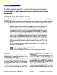
To derive the projection equations used in this research let us assume a volumetric object composed of a material with emission function C(x,y,z) and attenuation function µ(x,y,z). Then a ray emanating from a source with initial energy C0, traversing the object and collecting in bin (u,v) of a detector oriented at angle φ will have energy Cφ(u,v) (see Fig. 1): s
L
Cϕ (u, v) = ∫ C (s ) ⋅ e
∫
− µ ( t ) dt 0
rewrite the integral equation in an alternative, voxel-centric form: where the vj are the values for the reconstructed voxels (Cj or µj) at (x,y,z) and the wij are the weights with which the values of the vj contribute to the pixels pi. We can re-write the update
pi =
N 3 −1
∑ (v j =0
⋅ wij )
(2) 3
for a specific voxel vj, 0 ≤ j < N , as follows: Note that the meaning of the weight factors wij varies depending on the reconstruction algorithm used. In a Feldkamp-type grid update equation, a weight factor wij is the
L
ds + C0 ⋅ e
∫
− µ ( t ) dt 0
(1)
vj = vj +
∑ (p ⋅ w ) i
(3)
ij
pi ∈Pϕ
0
where s and t are parametric variables defined along the ray, and L is the distance between source and detector bin. In the following discussion, we will denote Ci = Cφ(u, v) for 0 ≤ i < M , where M is the total number of pixels (rays) in the acquired projection set. These pixels will be organized into images Pφ acquired at detector angles ϕ k , 0 ≤ k < S , where S is the total number of acquired projection images.
or ect det
Radionuclides(C) Attenuating object(µ) L
X-ray source
j
product of the interpolation weight for each pixel pi in the projection images and a depth weighting factor. On the other hand, the iterative method of Expectation Maximization (EM) [7] has the following grid update equation:
vj pi vj = 3 ∑ wij pi∈Pset N −1 ∑ ∑ vl wil pi ∈Pset l =0
w ij
(4)
We can rewrite this equation in terms of grid correction factors di:
vj =
∑ d i wij ∑ wij pi∈Pset
vj
(5)
pi ∈Pset
Figure 1: Transmission and emission imaging. An external X-ray source emits X-rays and internal radionuclides emit photons at sites of biochemical (metabolic) activity. Both are attenuated by the object’s densities.
We can decompose the reconstruction problem into two parts: first estimating the attenuation function µ(x,y,z) and then estimating the emission function C(x,y,z). To estimate µ let us assume that the Ci are free of contributions from emissive sources. Then we can rewrite the second part of (1) as follows: L
pi = ∫ µ (t )dt 0
where
C pi = − log i C0
The first part of (1) will be reconstructed once µ is known, using a hardware-implementable formulation that will be derived in the full paper. Since it is our goal to reconstruct a discrete grid of voxels, with values for emission C and for attenuation µ, it helps to
The term in the denominator of (4) in the most-inner bracket is a projection operator, where the wij can just be the voxel weights, or the combined voxel/attenuation weights, if one would like to incorporate the attenuation effects of the volume. The grid update factors di are computed and backprojected into the grid, using the same wij than in the projection step. A normalization step follows after all updates have been backprojected (thus a temporary accumulation volume for weights and updates is needed), and the result is multiplied (not added as in SART or Feldkamp) by the current voxel value. The procedure for OS-EM is very similar, just operating on a smaller set of projections. Thus all algorithms can be decomposed into very similar main elements, i.e., a set of projection and backprojection operations. The outcomes of these operations may be combined in different ways with simple arithmetic operations, such as multiplications and additions, on both the pixel level (to compute the grid corrections delivered by each ray) and on the voxel level (to compute the individual voxel updates), and a normalization step may be required. But all of these additional (glue) operations can be implemented in the latest
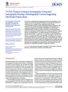
generation of GPUs. The incorporation of attenuation correction is achieved by maintaining an attenuation integral during projection and backprojection to composite the wij. GPUs give us a choice of 2D textures and 3D textures to store a volume, but only 2D texture stacks allow the backprojection operation. We therefore use two stacks of 2D textures, one for each of the two major viewing directions implied by a circular orbit. In the iterative algorithms, our use of two stacks of 2D textures will lead to inconsistencies if one stack of textures is updated by ways of backprojection but the other is not. Therefore we must update a texture stack whenever its projection proceeds an update of the other texture stack. This is frequently the case since two subsequent projections should be close to orthogonal to maximize the rate of convergence. By using a tiled texture, this texture stack compounding can also be performed rapidly in hardware. III. RESULTS First, we reconstructed the 3D Shepp-Logan phantom, on the usual 1283 grid. We used Feldkamp and 3 iterations of SART and 80 projections (see Fig. 2, left column). We see that all features, even the small tumors on the bottom, have been captured. We also reconstructed a CT head volume. We employed a high quality projection algorithm to simulate a set of 80 projections, and used SART to reconstruct. The results are shown in Fig. 2 in column 2 and 3. We used a simple hardware volume renderer without shading for the 3D rendering. To illustrate the reconstruction differences, we used the same transfer functions for both original and reconstructed volume, but we could obtain very similar images if we changed one of the transfer functions slightly. The slice images show that the reconstructions are quite accurate, with a slight low passing effect, as one might expect. Table 1 gives some insight into the reconstruction speed we were able to accomplish. Right now, we can perform a reconstruction of a 1283 volume with the FDK algorithm on the GeForce FX in seconds, and with the iterative algorithms in less than a minute, with 80 projections. We also found that these times scale linearly with the size of the dataset. Compared to a software implementation that uses raycasting, the present hardware implementation is already about 20 times faster. We expect the timings to improve as the drivers become more efficient. Algorithm Projection Backproj. 1 iteration Complete FDK 6s 7s SART 5s 6s 12s 36s EM-OS 5s 12s 19s 57s 3
Table 1: Timings for our reconstructions of a 128 volume with 80 projections and, for the iterative algorithm, 3 iterations. The EM uses full attenuation correction.
(a)
(b)
Figure 2: (Left): Shepp-Logan phantom reconstructed in hardware with (a) Feldkamp and (b) SART; (Center) Volume rendered CT head: (a) original, (b) reconstructed. (Right) Slices of CT head: (a) original, (b) reconstructed.
IV. ACKNOWLEDGEMENTS We thank Breakaway Imaging, Inc. for partially sponsoring this research. V.
REFERENCES
[1] A.H. Andersen and A.C. Kak, “Simultaneous Algebraic Reconstruction Technique (SART): a superior implementation of the ART algorithm,” Ultrason. Img., vol. 6, pp. 81-94, 1984. [2] B. Cabral, N. Cam, and J. Foran, “Accelerated volume rendering and tomographic reconstruction using texture mapping hardware,” 1994 Symposium on Volume Visualization, pp. 91-98, 1994. [3] L.A. Feldkamp, L.C. Davis, and J.W. Kress, “Practical cone beam algorithm,” J. Opt. Soc. Am., pp. 612-619, 1984. [4] R. Gordon, R. Bender, and G.T. Herman, “Algebraic reconstruction techniques (ART) for three-dimensional electron microscopy and X-ray photography,” J. Theoretical Biology, vol. 29, pp. 471-481, 1970. [5] H. Hudson, R. Larkin, “Accelerated Image Reconstruction Using Ordered Subsets of Projection Data,” IEEE Trans. Medical Imaging, vol. 13, pp. 601-609, 1994. [6] K. Mueller and R. Yagel, "Rapid 3D cone-beam reconstruction with the Algebraic Reconstruction Technique (ART) by using texture mapping hardware," vol. 19, no. 12, pp. 1227-1237, IEEE Trans. on Medical Imaging, 2000. [7] L. Shepp, Y. Vardi, “Maximum likelihood reconstruction for emission tomography”, IEEE Trans. on Medical Imaging, vol. 1, pp. 113-122, 1982. [8] L. Zheng, G. Gullberg, “Three-dimensional iterative reconstruction algorithms with attenuation and geometric point response correction,” IEEE Trans. on Nuclear Science, vol. 38, pp. 693-702, 1991.