Towards efficient vision-based object tracking ... - Computing Science

Towards efficient vision-based object tracking algorithms: rehabilitating visual information in particle filtering P´ eter Torma Ph.D. Thesis Supervisor: Csaba Szepesv´ ari, Ph.D.

Eötvös Loránd University Faculty of Informatics Informatics Ph.D. School Foundations and Methods in Informatics PhD Program János Demetrovics D.Sc. Budapest, 2007

ii ...for my kids Viola and Noémi ...to Junko, Mom and Dad

Acknowledgement Firstly I am grateful to my supervisor Csaba Szepesvári, not only for introducing me to many principles of machine learning, stochastic processes and AI, but also for teaching me how to research. I think my luck of having him as an advisor has the greatest impact on my motivations to analyze new ideas not only experimentally, but also in a mathematically rigorous way. This brings a better understanding of the structure of the problem, and usually helps further developing the theory while certainly useful in developing applications as well. I have learned that the symbiosis of engineering work, theoretical analysis, and experimenting forms an excellent base of research. Thank you, Csaba! The first lecture I took on AI has been Visual Illusions by Péter Aszalós. My inspiration of creating algorithms that aim to solve problems the human visual system does, was born there. Thanks for this enthusiastic lectures! Besides Péter, I am also thankful to András L˝orincz for introducing me to the field of modeling the human visual cortex. I would like to thank to companies I worked for. They involved me in inspiring engineering tasks, and allowed me to concentrate on their theoretical background as well. I am thankful to Zoltán Horváth, who was the leader of Mindmaker Ltd. and Morita Tsuneo, who is directing Tateyama Hungarian Laboratory Ltd. My thanks goes to László Balázs leader of GusGus AB Hungarian Branch Office, for teaching me a lot on organizing scattered thoughts nicely. This is always a great help in systemizing my ideas, both in research and programming. Lastly I can only admire my family. My mother, who always pushed and encouraged me in my Ph.D. work, my father who has been supportive in all aspects of my life, my lovely wife Junko, and kids Noémi and Viola for a lots of things that means family to me.

iii

iv

ACKNOWLEDGEMENT

Notation General P(U ) E(X) Var(X) x ∼ p() w ∝ f (x) F (f ) (f ∗ g)(x)

The probability of event U . The expectation of probability variable X. The variance of probability variable X. x is drawn from density p(·). R equals to cf (x), typically c = ( f (x)dx)−1 . The Fourier transform of f . Convolution of f and g.

Tracking Model X Y Xt , Zt Yt r(Yt = y|Xt = x) K(Xt = z|Xt−1 = x) M = (K, r) π(Xt = z|Xt−1 = x, Y0:t ) qX,Y (Zt = z)

State space of tracking. Observation space. Probability variables (over X ); object’s state at time t. Probability variable (over Y); observation signal at time t. Observation density, where x ∈ X . R Dynamics (x, z ∈ X ); K(z|x)dz = 1. A tracking model defined by a dynamical and an observation model. The (global) importance function used in importance sampling. The local importance function at z. The function also depends on the latest observation and particle position. pM (Xt |Y0:t ) The posterior of Xt given all observations.

Particle Filtering (i)

(i)

Xt , Zt (i) wt (i) (i) St = {(Xt , wt )}N i=1 N Neff

i-th particle at time t. The weight of the i-th particle at time t. The particle representation at time t. Number of particles. Effective sample size. v

vi

NOTATION

Abbreviations CONDENSATION iCONDENSATION SIR N-IPS AVM AVPF JPDAF HS-SIR RB-HS-SIR SS-RB-HS-SIR LS-N-IPS LLS LIS

Conditional Density Propagation Conditional Density Propagation with importance sampling Sequential Importance Resampling N-Interacting Particle System Auxiliary Variable Method Auxiliary Variable Particle Filter Joint Probabilistic Data Association Filter SIR with History Sampling Rao-Blackwellised SIR with History Sampling Rao-Blackwellised Subspace SIR with History Sampling Local Search N-Interacting Particle System Local Likelihood Sampling Local Importance Sampling

Contents Acknowledgement

iii

Notation

v

1 Introduction 1.1 Motivation . . . . . . . . . . . . . . 1.2 The Filtering Problem . . . . . . . 1.3 Example Tracking Problems . . . . 1.3.1 Contour Tracking . . . . . . 1.3.2 License Plate Tracking . . . 1.3.3 Bearings Only Ship Tracking 1.4 Thesis Overview . . . . . . . . . . .

. . . . . . .

. . . . . . .

2 Particle Filtering Elements 2.1 The Bayesian Solution . . . . . . . . . 2.2 Introducing Particle Representations . 2.3 Importance Sampling . . . . . . . . . . 2.4 Effective Sample Size . . . . . . . . . . 2.5 Resampling . . . . . . . . . . . . . . . 2.5.1 Degradation due to Resampling 2.6 The Bootstrap Filter . . . . . . . . . .

. . . . . . .

. . . . . . .

. . . . . . .

. . . . . . .

. . . . . . .

. . . . . . .

. . . . . . .

. . . . . . .

. . . . . . .

. . . . . . .

. . . . . . .

. . . . . . .

. . . . . . .

. . . . . . .

. . . . . . .

. . . . . . .

. . . . . . .

. . . . . . .

. . . . . . .

. . . . . . .

. . . . . . .

. . . . . . .

. . . . . . .

. . . . . . .

. . . . . . .

. . . . . . .

3 Importance Sampling in Particle Filtering 3.1 Sequential Importance Resampling (SIR) . . . . . . . . . . . . 3.2 SIR with History Sampling . . . . . . . . . . . . . . . . . . . . 3.2.1 Problem Setting . . . . . . . . . . . . . . . . . . . . . . 3.2.2 SIR with History Sampling . . . . . . . . . . . . . . . . 3.2.3 Rao-Blackwellised SIR with History Sampling . . . . . 3.2.4 Rao-Blackwellised Subspace SIR with History Sampling 3.2.5 Experiments with Contour Tracking . . . . . . . . . . . 3.2.6 Discussion . . . . . . . . . . . . . . . . . . . . . . . . . vii

. . . . . . .

. . . . . . .

. . . . . . . .

. . . . . . .

. . . . . . .

. . . . . . . .

. . . . . . .

. . . . . . .

. . . . . . . .

. . . . . . .

. . . . . . .

. . . . . . . .

. . . . . . .

. . . . . . .

. . . . . . . .

. . . . . . .

. . . . . . .

. . . . . . . .

. . . . . . .

1 1 4 5 5 7 10 12

. . . . . . .

15 15 16 17 17 18 19 20

. . . . . . . .

23 23 24 24 26 29 31 31 32

viii

CONTENTS

4 Local Perturbations in Particle Filtering 4.1 Motivation . . . . . . . . . . . . . . . . . . . . . . . . . . . . . . 4.2 Literature Overview . . . . . . . . . . . . . . . . . . . . . . . . 4.3 The LS-N-IPS Algorithm . . . . . . . . . . . . . . . . . . . . . . 4.3.1 Implementing Local Search for Contour Tracking . . . . 4.3.2 Experimental Results on the Contour Tracking Problem 4.4 Local Likelihood Sampling . . . . . . . . . . . . . . . . . . . . . 4.4.1 Theoretical Analysis . . . . . . . . . . . . . . . . . . . . 4.4.2 Inside LLS . . . . . . . . . . . . . . . . . . . . . . . . . . 4.4.3 LLS based Particle Filtering . . . . . . . . . . . . . . . . 4.5 Local Importance Sampling . . . . . . . . . . . . . . . . . . . . 4.5.1 Theoretical Analysis . . . . . . . . . . . . . . . . . . . . 4.5.2 Implementing LIS for Japanese License Plate Tracking . 4.5.3 License Plate Tracking Results . . . . . . . . . . . . . . . 4.5.4 Using Gauss-Mixture Proposals in LIS Filters . . . . . . 4.5.5 Experiments on the Bearings Only Problem . . . . . . .

. . . . . . . . . . . . . . .

. . . . . . . . . . . . . . .

. . . . . . . . . . . . . . .

. . . . . . . . . . . . . . .

. . . . . . . . . . . . . . .

. . . . . . . . . . . . . . .

5 Summary A Low Variance Resampling Methods A.1 Degradation of Multinomial Resampling A.2 Residual Resampling . . . . . . . . . . . A.3 Stratified Resampling . . . . . . . . . . . A.4 Systematic Resampling . . . . . . . . . .

39 39 41 42 43 46 47 49 54 55 59 59 61 63 63 66 81

. . . .

. . . .

. . . .

. . . .

. . . .

. . . .

. . . .

. . . .

. . . .

. . . .

. . . .

. . . .

. . . .

. . . .

. . . .

. . . .

. . . .

. . . .

. . . .

83 83 84 85 85

B Auxiliary Variable Method

87

C Partitioned Sampling

91

D Products of Gaussian Densities

97

Chapter 1 Introduction 1.1

Motivation

According to the legend “all this” started in the early 1960s when the Hungarian researcher, Rudolf Kalman, visited the NASA Ames Research Center. He realized the applicability of his ideas to the problem of trajectory estimation that came up in the Apollo program. His algorithm [17, 32, 16] soon became the main object tracking principle for many coming years. Applications were soon discovered by engineers in different areas, and the Kalman filter became the standard method of choice in designing aircraft autopilots, dynamic positioning system of ships, radar tracking and satellite navigation systems. In the trajectory estimation problem there is an observer equipped with some sensors that gather information about the state of the object to be tracked. The sensor can really be anything that provides relevant information on the object. A GPS sensor in navigation and a height sensor in aircraft autopilots are natural choices. The aim that Kalman settled is to use these sensory readings (also called measurements or observations) to the greatest possible extent to give the best estimation of the object’s pose. The sensors are assumed to supply noisy observations of the environment. A common suggestion is to treat the sensor noise independent in time. The object’s state and the sensor readings are connected through the observation model. Without any further information, the best estimate of the object’s state should be calculated using only the last sensor readings from the observation model. In particular the estimate would be independent of the previous observations. Naturally, this could lead to zigzagging object trajectories, which contradicts our expectations that objects move in a smooth manner. More reasonable trajectories can be obtained by making this expectation part of the model by assuming a motion model. As a result one gets smoother object trajectories. In summary, the object model has two parts: the motion or dynamical model provides predictions for the object’s next state given the previous state, while the sensor or observation model describes the relation between the sensory readings and the object’s state. The filtering task is to give the best estimate of the object’s state assuming that the observations comply with the assumed model. When assuming probabilistic models and an initial distribution for the object’s state for the time 1

2

CHAPTER 1. INTRODUCTION

step before the first observation arrived, the solution is given by the posterior distribution given the observations. The actual utility of the posterior is limited by the correctness of the models. As an example assume that one receives a sequence of GPS sensory readings with the task of estimating the trajectory of an object moving on the earth in a certain geographical region. Clearly, a simple auto-regressive motion model will lead to estimated trajectories which can be quite different from those obtained by assuming a model that uses road maps. Similarly, different sensor models will certainly lead to different estimates. In the case of GPS sensors, the model of the sensor noise becomes an issue as different noise models lead to different estimates. Hence, one should never forget that the estimates depend not only on the observations, but also the models assumed. It is reasonable to assume that our brain uses both observation and motion models. As an example, imagine that you would like to catch a flying badminton shuttlecock. The weather is windy and the sun shines into your eyes. How does your brain knows how to move your hands? Due to air turbulence, it would certainly be hard to guess the exact landing position just by watching the moment of throw, and closing your eyes after that. It is harder to imagine, but sounds more obvious that only using your eyes and not your brain would be inefficient for catching the ball. Now, during the play the sun suddenly comes out from behind the clouds, shines into your eyes, reducing the quality of visual information drastically. Our brain helps us through these situations by not only estimating the position of the shuttlecock, but its speed and direction of motion as well, by effectively modeling the motion of the objects tracked. As we discussed earlier, the dynamical model is meant to describe how the object generally moves from one time step to the next. This implies that the state should be a sufficient statistic for the object’s future observations. In other words the state space and the dynamical model should be designed in such a way that the dynamical model is Markovian over the state space. One should prefer low dimensional state spaces, since estimation in high dimensional spaces is harder. Achieving sufficient precision then requires careful engineering. However often the preference to low dimensionality means that many physical effects stay un-modeled (e.g. the spinning of the shuttlecock, or how the wind blows in the above example). A particularly popular choice is to model the dynamics using a low-order auto-regressive process. Our main interest is to construct algorithms that track the object’s state well over time. Kalman filters are designed to work with the so-called linear Gaussian models. For such systems, the posterior is Gaussian whose parameters can be calculated in a recursive (and thus cheap) manner. It is, in fact, this algorithm that is called the Kalman filter. Unfortunately in several important trajectory estimation problems linear Gaussian models are inappropriate. The Extended Kalman Filter [36] and the more recent Unscented Kalman Filter [35, 52] represents one line of research that are designed to work for nonlinear and/or non-Gaussian systems. Although these methods extend the scope of Kalman filters considerably, they are fundamentally limited to problems were the posterior is unimodal. In several problems the available observations are often insufficient to rule out multiple significantly different hypotheses, hence one needs a tool capable of representing such multimodal posteriors. Particle filters are designed to handle such situations.

1.1. MOTIVATION

3

The development of particle filters goes back to the early 50s, but their intensive study started during the past 10 years. The original idea can be traced back to Metroplis and Ulam [27]. An early summary is given by Rubinstein [11]. The rebirth in the past decade was due to a review paper by Doucet [9] followed by the seminal papers of Kitagawa [18] or Liu [21]. In computer vision an algorithm called CONDENSATION means the starting point [14, 2]. The key idea in particle filtering is to use a discrete non-parametric representation PN for the posterior, i=1 w(i) δ(x − X (i) ), where the weights wi are non-negative and sum to one and δ is the Dirac-delta distribution function. This representation is hierarchical in its nature, since the particle positions determine the importance weights as well.1 It follows hence then that particle filtering algorithms should concentrate mainly on locating the particles to valuable positions. However, most of the particle filtering algorithms determine the particle positions using only the dynamical model and the prior (Bootstrap Filter), or only the most recent observation (likelihood sampling, SIR with observation based importance function). The questions investigated in this Thesis are: a) What is the best way to let the dynamical model influence the particle locations in SIR when the proposal function depends only on the observation? b) How to let the latest observation influence the dynamical model based state prediction in the Bootstrap Filter? In this Thesis the sensor observing the environment will be a video camera. The observation signal is then the image frame. Problems with this setup are called visual tracking problems. There are several specialties of this type of tracking problems. An image as a measurement signal of the environment is a complicated one. Extracting position information of objects from images is usually a challenging image processing task. Furthermore since the complicated rules of camera optics and image projection, the object’s motion model is usually kept very simple. We will assume that evaluation of the observation likelihood has the highest computational cost. This is why we will try to keep the number of observation density evaluations low. An important reason why particle filtering is particularly appealing in visual tracking lies in the fact that the the images has to be processed only in the neighborhood of the predicted particle locations. This can be a great advantage compared to other image processing based tracking algorithms, when all the image frames has to be fully scanned for the search of objects. As a result, using particle filtering not only leads to better trajectory estimates, but also a faster algorithms. At the same time observations coming from image-processing steps are usually more reliable than the state predictions arising from the dynamical model. As a result the observation likelihood function becomes ‘peaky’ (comparing to the prediction density) or 1

More exactly, the particle positions determine the expected value of the weights, but in most of the algorithms the weights are fully determined by the particle positions and hence the weights are equal to the above mentioned expected value. An exception besides some of the algorithm introduced in this Thesis is the Auxiliary Variable Method [31], where only the expected value of the weights are determined.

4


concentrated around its modes (the modes correspond to the states that are locally most likely to ‘cause’ the past observations). If the position of a particle is not sufficiently close to one of these modes then the corresponding weight will bring in little information on the estimate of the posterior. As an analogue to Bellman’s curse of dimensionality, we shall call this problem, particularly eminent in visual tracking, the “curse of reliable observations”.

1.2

The Filtering Problem

In this section we give a formal description of the filtering problem. From a mathematical viewpoint the problem is to estimate the state of a discrete time, partially observed stochastic system evolving in time. In this Thesis the dynamical model will be defined by a kernel function K(xt |xt−1 ) which gives the probability density of the object’s state xt ∈ X at time t given the object’s state xt−1 ∈ X at time t − 1. If one has a density of the object’s state at time t − 1, say pt−1 (xt−1 ), then the state-density for the next time step can be given as Z pˆt (xt ) = K(xt |xt−1 )pt−1 (xt−1 )dxt−1 . At each time step an observation signal is received from the sensors that depends on the object’s current state only. Let us denote the observation signal at the t-th time step by Yt ∈ Y, where Y is the observation space. The choice of the observation space mainly depends on the sensors observing the system to be tracked. For example, in the case of a satellite navigation system with a GPS it includes the latitude, altitude and longitude. In the case of visual tracking it is the observed image frame. The observation model is required to give a distribution of the observation signal given the object’s state. In this Thesis the observation density will be denoted by r(yt |xt ). It is by assumption that this density is only a function of xt . Hence if one has a density of the object’s state at time xt denoted by pˆt (xt ) then the density for the observation at the corresponding time step is: Z rˆt (yt ) = pˆt (xt )r(yt |xt )d(xt ). Another way of viewing this model is to say that at time t the new state is assumed to be sampled from K(·|Xt−1 ), while the new observation signal Yt is sampled from r(.|Xt ). Such models are called Hidden Markov Models [3]. In the literature it is a common practice to denote both the dynamical kernel and the observation density by p and leave it only to the arguments to define the function under consideration. A common further overloading of the symbol p is to use it to denote the prediction and/or posterior densities. The reason we make an effort to avoid this is to make it clear that we work with models of the motion and observation, which do need to match “reality”. Whenever appropriate a sub-index M = (K, r) referring to the model will be used to signify when a density depends on the assumed model.

1.3. EXAMPLE TRACKING PROBLEMS

5

The tracking problem is to compute the posterior density: pM (Xt |Y0:t ), where we have used the convention Y0:t = Y0 , . . . , Yt . By definition the posterior describes the density of the object’s state given all available observations. When the model under consideration is unimportant we will omit the index M .

1.3

Example Tracking Problems

In this section we introduce some vision-based tracking problems to motivate the further developments. These problems will serve as testbeds in the rest of the Thesis.

1.3.1

Contour Tracking

The problem is to track an object contour on a video frame. For simplicity the dynamical model assumes that the shape of the object’s contour changes only slightly, except for its size and rotation which are free parameters. Figure 1.1 shows some example frames of a video sequence, while an example contour with its B-spline control points is shown in Figure 1.2. We assume that the object does not disappear, and no similar objects enter the scene. The object might however make sudden movements and the scene lighting conditions might change. State Space The state space consists of the pose of the object to be tracked along with the previous pose. This is because the motion model uses the speed of the object as well. More exactly the motion model is a second order auto regressive model on the object’s pose. A pose defines a contour mapped onto the camera plane (i.e., onto the image) and observations will be defined in terms of contours and the observed images. A contour is represented by a B-spline [43]. Let us consider the spline curve s : [0, L] → 2 R defined by its support points (which lie on the curve) q x = (q1x , . . . qnx )T , q y = (q1y , . . . qny )T , i.e: s(t) = ((A−1 q x )T ϕ(t), (A−1 q y )T ϕ(t)), where ϕ(t) = (ϕ1 (t), ϕ2 (t), . . . , ϕn (t))T are the usual B-spline basis functions (cf. [2]) and s(i) = (qix , qiy )T . A is linear transformation mapping control points to support points and depends only on ϕ. Let q0 = ((q0x )T , (q0y )T ) ∈ Rk be a vector of support points defining the template contour s0 = S(q0 ) ⊂ R2 . If G is a group of similarity transformations of the 2D plane (R2 ) then one can find a matrix W = WG,q0 such that T ∈ G iff for some z ∈ Rd , d ≥ 1, the support vector q = W z + q0 yields the spline curve T s0 , or S(W z + q0 ) = T s0 . Here we use the convention that z = 0 corresponds to T = Id. Thus, if G represents the set of admissible transformations of the contour then the set of admissible object configurations will correspond to Rd .

6


Figure 1.1: Frames of a contour tracking problem video together with the sample desired results (white contours).

Figure 1.2: An example contour with its B-spline control points.


7

Figure 1.3: An example contour with its B-spline control points and a measurement line(black) used in the observation likelihood calculation. We will use the group of Euclidean similarities of the plane. Thus in this Thesis d = 4 and 1 0 q0x −q0y , (1.1) W = 0 1 q0y q0x where 0 = (0, 0, . . . , 0)T , 1 = (1, 1, . . . , 1)T are of the appropriate dimensions. Observation Assume that a contour (s) corresponding to some pose (z) is given. The following observation model is due to Blake and Isard [14]. They define the likelihood of the observed image given a pose by assuming that the image is formed such that edge positions along measurement lines perpendicular to the contour follow Gaussian-distribution and edge positions at different measurement lines are independent of each other. Figure 1.3 shows a sample contour with a selected measurement line.

1.3.2

License Plate Tracking

In this problem tracking of Japanese license plates is considered. Japanese license plates have a fixed geometrical layout, which is very helpful in constructing a reliable observation model. Figure 1.4 shows some example frames of a video sequence. The cars appear on one side of the image and disappear at the other end. The cars entering the scene must be detected and tracked all the time when they are visible. State Space The license plate (LP) area can be represented by a parallelogram with two vertical lines and a fixed aspect ratio. Hence the configuration of a LP is defined through four parameters. In the followings we will denote these by u, w, and θ, where u and w correspond to the horizontal and vertical position of the center of the LP on the image, while θ ∈ [0, π) × [0, +∞) determines the angle of the non-vertical side and the scale of the parallelogram. The state space is twice the size of the pose-space, again assuming a second order dynamics: x = (unow , wnow , θnow , uprev , wprev , θprev ).

8


Figure 1.4: Frames from a Japanese license plate tracking video. Dynamical model The dynamical model is a mixture of Gaussians. There is a Gaussian that is responsible for representing new cars entering the scene. This Gaussian has a weight of 0.1. Otherwise the state evolves according to a simple AR(2) model. The AR(2) is factored: the middle of the license plate, the size, the orientation and the rate of the parallelogram sides all develop independently of each other. Strictly speaking, independence does not hold in practice, the choice of this model stems from our desire to minimize the number of free parameters and hence to increase the robustness of the model. The parameters of the AR models were selected by hand in a manner so that the variance of the process noise is overestimated. This was also meant to increase robustness against unexpected movements. Observation model In the followings we will refer to a configuration (or pose) as (u, w, θ). Now, we define the observation model given a configuration. Japanese license plates enjoy a very restricted geometrical structure, as shown in Figure 1.5: The three main character areas are always positioned at the same place and areas between them remain free of edges. This gives the basic idea of our observation model. The likelihood itself is expressed as the product of three likelihood functions that correspond to three different qualities of the LP. The best way to describe the way these individual likelihoods are computed is to introduce a number of categories and pixel-sets. Consider the categories and pixel sets listed in Table 1.1. For each specific area the likelihood is determined so that it results in a big value if the image looks ‘right’ over that given area. When checking if an image looks ‘right’ we look for the absence or presence of edges and lines over the appropriate areas. For detecting edges we use the Sobel operators.


Category Area of horizontal edges Horizontal stripes free of edges and lines Area of vertical edges Vertical stripes free of edges and lines Area of small characters Area of large characters

9

Pixel set Sign in Figure.1.5 P (u, w, θ) solid line h,f e P (u, w, θ) dashed line v,e P (u, w, θ) solid line P v,f e (u, w, θ) dashed line P sc (u, w, θ) dotted bc P (u, w, θ) checked h,e

Table 1.1: Categories of license plate parts and symbols denoting the corresponding pixel sets.

Figure 1.5: A Japanese license plate (left) and its template model (right): The area of large characters is checked, the area of small characters is dotted. The system of horizontal and vertical edge and line-free stripes is marked by dashed lines, whilst stripes of horizontal and vertical lines is marked by solid lines.

10


The corresponding horizontal (vertical) edge images shall be denoted by ∇x I (resp. ∇y I). For evaluating line features the image was convolved with 2D difference of Gaussians (DOG) filters approximated by the difference of two 2D box-filters having different scales. Two such filters are needed, one with a larger scale (for detecting lines on thick characters) and one with a smaller one (to detect lines of thin characters). The corresponding processed images will be denoted by Gs I and GS I, corresponding to the smaller- and larger-scale lines, respectively. The likelihood that a given image y = I is generated by a license plate of configuration (u, w, θ) is thus computed as r(y|u, w, θ) = rh (y|u, w, θ) rv (y|u, w, θ) rc (y|u, w, θ), where the likelihoods rh , rv and rc are defined through their logarithms as follows: X 1 |(∇x I)(p)| − log rh (y|u, w, θ) ∝ #P h,e (u, w, θ) h,e p∈P

1 #P h,f e (u, w, θ) log rv (y|u, w, θ) ∝

1 v,e #P (u, w, θ)

1 sc #P (u, w, θ) 1 bc #P (u, w, θ)

|(Gs I)(p)| + |(GS I)(p)|

p∈P h,f e (u,w,θ)

X

|(∇y I)(p)| −

p∈P v,e (u,w,θ)

1 v,f e #P (u, w, θ) log rc (y|u, w, θ) ∝

(u,w,θ)

X

X

|(Gs I)(p)| + |(GS I)(p)|

p∈P v,f e (u,w,θ)

X

|(Gs I)(p)| +

p∈P sc (u,w,θ)

X

|(GS I)(p)|.

p∈P bc (u,w,θ)

The symbol #P denotes the cardinality of the set P. These various sets have been introduced in Table 1.1. By inspecting a large number of images we have found that the proposed likelihood function is successful at discriminating plates and clutter: it has a single dominant peak at the location of the true plate or plates. Figure 1.6 shows a typical landscape of the likelihood as a function of u and w. Certainly this observation model could be further refined by e.g. learning coefficients for each of the terms.

1.3.3

Bearings Only Ship Tracking

In contrary to the previous problems, in this section we will examine a simulated example. This implies that we know the object’s exact dynamical and observation model. The problem is a standard one that has been considered previously by several authors [13, 31, 4, 1]. The aim is to track the (horizontal) motion of a ship, while observing only angles


11

Figure 1.6: The observation likelihood (right) function for the frame shown (left). Note that the highest peak has a pretty small support, i.e. the observation likelihood function is sensitive to the precise positioning of the license plate. This is a desirable property if the goal is to determine the license plate’s position with high accuracy. The scale and the orientation are selected to match their corresponding true values. to it. We assume that the coordinate system is fixed to the observer. The ship’s state is assumed to follow a second order AR process, with its acceleration driven by white noise:     1 1 1 0 0 0 2  0 1 0 0   1 0   ξ,   Xt+1 =  X + 0 0 1 1  t  0 12  t 0 1 0 0 0 1 where Xt , ξt ∈ R2 , ξt1 , ξt2 ∼ N (0, 1), and Xt1 , Xt3 represent the ship’s respective vertical and horizontal positions, whilst Xt2 , Xt4 represent the ship’s vertical and horizontal velocities. The initial state is sampled from a 4-dimensional Gaussian with a diagonal covariance matrix. What makes this problem particularly challenging is that the observations depend on the state only through the angle, θt = tan−1 (Xt3 /Xt1 ), at which the ship is observed. The observation noise is defined by a “wrapped” Cauchy density: r(y|θt ) =

1 1 − ρ2 . 2π (1 + ρ2 − 2ρ cos(y − θt ))

This density (when ρ is close to one) is thought to reflect well a sonar’s behavior: angle measurements are typically very reliable, whilst possible outliers are well modeled by the heavy tails of the wrapped Cauchy distribution. The parameters of the model used in the experiments are as follows: ση = 0.001, ρ = 1− 0.0052 , and the initial state is sampled from a Gaussian with means (−0.05, 0.001, 0.2, −0.055) and with a diagonal covariance matrix with diagonal entries given by 0.001 × (0.52 , 0.0052 , 0.32 , 0.012 ). Figure 1.7 gives an example of the ship’s motion and the observed angles.

12


Figure 1.7: An example of the ship’s motion in the bearings only tracking problem together with some rays representing the observations.

1.4

Thesis Overview

Let us now give an overview of the Thesis: In the next Chapter we first derive the exact solution to the filtering problem. Then we discuss the basic building blocks of particle filtering. Issues and important concepts are discussed, including resampling, importance sampling and the effective sample size. The main motivation of this Thesis is to show how the observation model can be better used in the particle localization stage of particle filtering. The obvious way of incorporating information coming from the observation is importance sampling. However it is common that the last observation does not hold information for all the components of the state space. For instance observing only the pose of the object might bring no information in view about the speed or the direction of motion. The straightforward importance sampling scheme then might result in poor approximations, since the likelihood of most of the particles might get very small as the history part of the new state is not associated with the observation based innovation content. In Chapter 3 we propose a solution that overcomes the problem. The proposed family of algorithms samples the particle’s history hence the algorithms are called history-sampling based particle filters. Chapter 4 describes a more complicated but an often more effective method to locate the particles that uses both the observation and the dynamical model. They key idea lies in a modification of the Bootstrap Filter, whereas the particles are re-allocated after they

1.4. THESIS OVERVIEW

13

are predicted using the dynamical model. This step, that we call the position perturbation step, is done by locally analyzing the observation likelihood around each predicted location and let the particles be dragged by the local modes of the observation likelihood. One can think of this idea as a particle localization procedure that uses the global behavior of the dynamical model combined with the local characteristics of the observation model to locate the particles. This combination is particularly appealing since in visual tracking the dynamical model is less reliable, and hence it is able to give valuable particle location regions only. In this sense the dynamical model gives good particle locations in a “low frequency” manner. In contrary the much more reliable observation gives focus to spots of good particle locations, providing them in a “high-frequency” way. It is shown that these methods increase the efficiency of particle filtering in case of reliable observation models. The text focuses on the theory of the algorithms, but experiments on the above tracking problems are also given. Although the ideas are explained in a general framework, this chapter is highly motivated by visual object tracking situations. In the Appendix several related advanced particle filtering algorithms are discussed using the notation of this Thesis. The reason that these algorithms are not detailed in the main body, is to keep the body focused on the new ideas.

14


Chapter 2 Particle Filtering Elements 2.1

The Bayesian Solution

The filtering problem formulated in Section 1.2 has an analytic solution that can be obtained by applying Bayes theorem, the law of total probability and exploiting the following independence assumptions: (i) The observation signal given the last state is independent of the previous observation signals: pM (yt |xt , y0:t−1 ) = pM (yt |xt ). (ii) The state is independent of the previous observation signals, if the previous state is given: pM (xt |xt−1 , y0:t−1 ) = pM (xt |xt−1 ). Then the posterior can be calculated, up to a proportional factor, as follows: pM (Yt |xt )pM (xt |Y0:t−1 ) pM (yt |Y0:t−1 ) Z ∝ pM (Yt |xt ) pM (xt |xt−1 )pM (xt−1 |Y0:t−1 )dxt−1 Z = r(Yt |xt ) K(xt |xt−1 )pM (xt−1 |Y0:t−1 )dxt−1 .

pM (xt |Y0:t ) =

(2.1)

Note that this is a recursive equation for pM (xt |Y0:t ). Thus, when the initial state density p0 (x0 ) is known, pM (xt |Y0:t ) can be computed via (2.1). Unfortunately, the exact solution cannot be computed except in a few special cases such as the case of linear Gaussian models or finite Hidden Markov models (in the former case the solution is given by the Kalman filter, while in the latter case it is given by the Baum-Welsch equations). In practice the models are often more complicated. Therefore a large body of current work in the filtering literature is devoted to finding the posterior in an approximate manner. 15

16

CHAPTER 2. PARTICLE FILTERING ELEMENTS

2.2

Introducing Particle Representations

As it was noted above, the exact solution of the filter evolution equation (2.1) is not feasible in general. One approach to overcome this problem is to use sequential MonteCarlo methods to sample from the posterior. The key issue here is to construct a weighted sample set that represents the posterior in a faithful manner. One approach is to target unbiased representations: Definition 2.2.1. A random variable X is said to be properly weighted by the function w with respect to the density p and the integrable function r if for any integrable function h, E[h(X)w(X)] = I(hrp), R where I(f ) f (x) dx is the usual integral operator. Alternatively, we say that (X, w(X)) forms a properly weighted pair with respect to p, r. A series of random draws and weights {(X (k) , w(k) )}k=1,...,N is said to be properly weighted with respect to p and r if all members of the set are properly weighted with respect to p and r. If {(X (k) , w(k) )}k=1,...,N are independent properly weighted samples with respect to p and r then by the law of large numbers the sample averages JN (h, w) = (1/N )

N X

h(X (k) )w(X (k) )

j=k

will converge to I(hrp) if it exists. Hence, in this sense, a properly weighted set with respect to f and r can be thought of as representing the product r(·)p(·). In this context h is an integrable test-function. Its form certainly affects the quality of the estimation, and hence the speed of convergence of JN (h, w) to I(hrp). (i) (i) Furthermore, if one is given a properly weighted sample-set (Xt , wt ), i = 1, 2, . . . , N from the posterior pM (Xt−1 |Y0:t−1 ) then an unbiased sample from pM (Xt |Y0:t ) can be generated by the following two-step method [9]: (i)

(i)

1. Prediction: Draw Xt from K(Xt = ·|Xt−1 ), i = 1, 2, . . . , N , (i)

(i)

(i)

2. Evaluation: wt = ct wt−1 r(Yt |Xt ), i = 1, 2, . . . , N . Here the unknown proportional factor ct is inversely proportional the the probability of the latest observation given the previous ones, i.e., ct = 1/pM (Yt |Y0:t−1 ). Note that ct depends only on the observations and does not depend on the particles’ properties. (i) Elements of the sample (Xt ) are traditionally called particles and the filtering method is called particle filtering [9].

2.3. IMPORTANCE SAMPLING

2.3

17

Importance Sampling

Importance sampling is an important Monte-Carlo estimation procedure. It suggests to estimate µ = Ep (h(X)) by N 1 X p(Xi ) µ ˆ= h(Xi ) π(X , i) N i=1 where X1 , . . . , XN are independent samples from a distribution π(·) satisfying that whenever p(x) > 0 then also π(x) > 0. The choice of π certainly influences the efficiency of the sampling to a great extent. A good choice of π is one that is close to |h(x)p(x)|. When π ∝ |hp| the variance becomes i )p(Xi ) = µ. If sampling from p(.) directly is difficult but generating from π zero, and h(Xπ(X i) and computing the importance ratio w(X) = p(X)/π(X) are easy, then using importance sampling might lead to an effective estimation procedure. A special choice of π is p itself. In this case the importance sampling scheme is identical to the simple Monte-Carlo integral estimation. Another useful variation of this idea is called weighted importance sampling. In this procedure we estimate µ by PN h(Xi )w(Xi ) . µ = i=1 PN w(X ) i i=1 This estimate is only asymptotically unbiased. This is easy to see by considering only one particle N = 1. The estimate becomes h(Xi ) independently of p, which is obviously biased in general. In contrary the simple importance sampling gives unbiased estimate even for a single particle. However in other performance measures such as E [(µ − µ)2 ) weighted importance sampling often outperforms importance sampling. Further note that this estimation works if one knows p only proportionally.

2.4

Effective Sample Size

The asymptotic consistency of a Monte-Carlo procedure represents only a minimal requirement that does not tell anything about the quality of the estimates. One way to measure the quality of a randomized estimate is to compute its variance: in our specific case one goal can be to obtain a properly weighted set such that the variance of the sample average JN (h, w) is minimized (or is small). Actually, we are more interested in studying the weight-normalized averages PN (j) (k) ) j=1 h(X )w(X IN (h, w) = (2.2) PN (j) j=1 w(X ) which, again under proper conditions, converge to the normalized value I(hrp)/I(rp) as N → ∞ with probability one. As mentioned before, in practise IN (h, w) is more preferred then JN (h, w), since its variance is smaller. On the other hand it is true that IN (h, w) is

18


biased for any finite N . Particle filters make use of these weight-normalized averages to represent the empirical measure. In this way they do not have to estimate the normalization constant ct , which is a significant advantage. Obviously, the variance of the sample average depends on h. Certainly we are interested in the case when h is not fixed. Liu [20] (based on [19]) shows that it is sensible to measure efficiency by a quantity inversely proportional to the variance of w(X), provided that w is such that E[w(X)] = 1. We will refer to this scheme as Liu’s ‘rule of thumb’. In turn this leads to a measure of efficiency Neff =

N , 1 + V ar(w(X))

which is called the effective sample size. If Neff = N , i.e, all weights are equal, then the optimal sampling strategy is implemented. In other words the particle locations are sampled exactly from the product r(·)p(·). Liu’s rule of thumb will serve as our starting point. In particular, since for any properly weighted pair (X, w), E[w(X)] = I(rp) and Var[w(X)] = E[w2 (X)] − E[w(X)]2 it follows that minimizing Var[w(X)] is equivalent to minimizing E[w2 (X)]. Therefore, it follows that it is sufficient to compare unbiased algorithms on the basis of the second moment of the weights they use, since it is the same as comparing Neff . Note that if X is drawn from p and w is set to be equal to r, as in the case of the sampling procedure underlying the two-step method of Section 2.2, then E[w2 (X)] = I(r2 p).

(2.3)

An empirical measure of the effective sample size follows from the fact that the estimate of the variance can be given as PN (w(i) )2 V ar(w(X)) = i=1 − 1. N Hence: êff = N

2.5

N 1 . = PN 2 (i) 2 E(w ) i=1 (w )

Resampling

The serious problem with the two-step method of Section 2.2 is that given any finite (i) sample size the weights wt will degenerate: in general all of them converge to 0 except (i) for one index, for which wt will converge to 1. This means that the observation model will have no effect on the sample trajectories, which hence becomes a simple random walk with the dynamical kernel K. In order to prevent this degeneration, a resampling step was introduced into the above procedure by Gordon et al. and Rubin [13, 34]. Given N a particle set (X (k) , w(k) ) i=1 the aim of resampling is to generate a new particle set

2.5. RESAMPLING

19

n oN ˆ (k) , wˆ (k) ) (X

with lower weight variance, most often equal weights. Since the only input of this method is the original particle set, the new particle positions are simply sampled from among the original ones. Certainly the new particle set should still be an unbiased estimator of the distribution in question. This can be ensured by considering random weights satisfying   X E wˆ (j)  = N w(j) i=1

ˆ (j) =X (j) j:X

We will mainly consider algorithms that generates equal weights, i.e: wˆ (j) = 1/N j = 1, . . . , N . The simplest resampling algorithm called Multinomial resampling is shown in Figure 2.1. For n = 1, 2, . . . , N Sample Ni from the multinomial distribution M ult(N ; w(1) , w(2) , . . . , w(N ) ). ˆ (i) = X (Ni ) and wˆ (i) = 1. Let X EndFor

Figure 2.1: The Multinomial Resampling. N is the number of particles and i = 1, 2, . . . , N is a particle index. It is easy to imagine that the resampling step made regularly solves the above mentioned degeneracy problem of particle filters, by always keeping the majority of the samples in valuable location. It is important to notice that resampling gave an important boost to sequential Monte-Carlo methods, and made the two-step procedure of Section 2.2 a practical algorithm [13]. However nothing comes for free. As it is shown in the next section resampling increases sampling variance.

2.5.1

Degradation due to Resampling

The following statements and proofs are mainly the work of Móri Tamás (personal communication). Imagine we have N particles all of them with equal weight (1/N ). Assume that not all of the particles are unique, but we only have m ≤ N distinct ones. Let their respective duplication numbers be N 1 , . . . N m . Let us define the duplication of the m distinct P weights 0 particles as W10 = N 1 /N, W20 = N 2 /N, . . . , Wm0 = N m /N ( m W = 1). Assume we i i=1 recursively resample the particle set with multinomial resamplings for a couple of times.

20


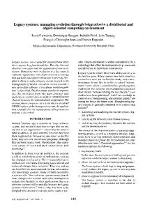
Figure 2.2: The expected degradation time of resampling as a function of particle number. Let Wi = (W1i , W2i , . . . , Wmi )T be the duplication weights of the particles after the i-th resampling. It is clear that N Wji+1 is drawn from an N -th order binomial distribution with parameter Wji , i.e: P(N Wji+1

N = k|Wi ) = (Wji )k (1 − Wji )N −k k

Let Tn be the time of reaching a completely degenerated particle that PN setk (meaning i there is a single particle having all the weights), i.e.: TN = inf{k| j=1 Wj (1 − Wj ) = 0}. In Appendix A.1 it is shown that ETN ≤ 2N log 2N . In fact Monte-Carlo experiments suggests that ETN is even linear in N . Results of Monte Carlo experiments when m = 2 are shown in Figure 2.2. Overall this suggests that degradation of a constant particle set with repeated multinomial resampling is very fast. Hence this procedure should be used with extra care. It should also be clear that it is a good idea to decrease the variance of the resampling scheme. Some popular low variance resampling methods are given in Appendix A. The paper [33] is an excellent summary of this issue.

2.6

The Bootstrap Filter

The Bootstrap Filter, also known as CONDENSATION [14] in the visual tracking literature, is the simple combination of the two-step method of Section 2.2 and resampling. The algorithm is shown in Figure 2.3. A visual representation is given in Figure 2.4.

2.6. THE BOOTSTRAP FILTER

21

h iN (k) Initialize (Z0 , 1/N ) from the prior p0 (·). k=1 For t = 1, 2, . . . For k = 1, 2, . . . , N h iN (j) (j) Resample (Zt−1 , wt−1 ) j=1 h i N (k) 0 (Zt−1 , 1/N ) .

to

obtain

a

new

sample

j=1

(k)

Sample Zt (k)

Let w ˆt

(k) 0

∼ K(.|Zt−1 ). (k)

= r(yt |Zt ).

EndFor Normalize weights using (k)

(k) wt

wˆt

= PN

i=1

(i)

wˆt

EndFor Figure 2.3: The Bootstrap Filter. N is the number of particles and i = 1, 2, . . . , N is a particle index.

22


Figure 2.4: Sampling in the Bootstrap Filter. Positions of the particles (represented by white circles in the upper part) are drawn from the prediction density. The particles are propagated through the observation likelihood density to produce a weighted sample. The radii of the black discs are plotted in proportion to the size of the weight corresponding to the respective particles. The lower subplot shows the product of the prediction and observation. Ideally, the ‘particle cloud’ composed of the black discs should closely reflect the shape of the posterior.

Chapter 3 Importance Sampling in Particle Filtering 3.1

Sequential Importance Resampling (SIR)

Using importance sampling in particle filtering goes back to [34, 40]. For some reason one wants to sample the proposed the next states from a so-called proposal density π(Xt = ·|Xt−1 , Yt ) instead of K(Xt = ·|Xt−1 ). The only restriction on this density is that π(xt |xt−1 , Yt ) > 0 whenever K(xt |xt−1 ) > 0. The derivation of the algorithm is again simple: Z p(Xt |xt−1 ) p(xt−1 |y0:t−1 )dxt−1 p(Xt |y0:t ) ∝ p(yt |Xt ) π(Xt |xt−1 , yt ) π(Xt |xt−1 , yt ) The simplest importance sampling based particle filtering algorithm, the so called Sequential Importance Sampling/Resampling (SIR) algorithm, is shown in Figure 3.1. Obviously, the choice of π effects the efficiency of the algorithm in a fundamental way. As in the general case, the best is certainly if π is close to the posterior itself. Note that the Bootstrap Filter itself is an importance sampling algorithm, with π(xt |xt−1 , Yt ) = K(xt |xt−1 ), i.e: the proposal does not depend on the latest observation signal. On the other hand in visual object tracking it is common to choose proposals that depend only on the last observation, and not on the previous state, i.e, π(xt |xt−1 , Yt ) = π(xt |Yt ). In these cases the proposal distribution is computed via some rough and fast image processing steps e.g: color blob detection or edge filtering, which proposes particle positions with possibly high observation likelihoods. In some cases the proposal is not well defined on all dimensions of the state space. This happens, e.g., if the state space holds some historical information on the particles, or the image processing involved in the proposal function is not defined on all the dimensions of the object’s pose, e.g. the color blob detector is usually not defined in the rotation component. In these cases the the proposed particle positions are not fully defined and hence the algorithm described in Figure.3.1 gets badly degraded. In this chapter we will discuss the particle filtering algorithms introduced in [48] that overcome these problems. 23

24

CHAPTER 3. IMPORTANCE SAMPLING IN PARTICLE FILTERING h

iN

(k) (Z0 , 1/N )

Initialize For t = 1, 2, . . .

k=1

from the prior p0 (·).

h iN (j) (j) Resample from (Xt−1 , wt−1 )

j=1

h iN (j) (j) ˆ t−1 if needed, to obtain (X , wˆt−1 ) . j=1

For k = 1, 2, . . . , N Sample from the proposal (k)

Xt

(k) ˆ t−1 ∼ π(.|X , Yt ).

Calculate the importance weight (k)

(k) wt

=

(k) (k) wˆt−1 r(Yt |Xt )

(k)

ˆ t−1 ) K(Xt |X . (k) ˆ (k) π(Xt |X t−1 , Yt )

EndFor Normalize weights using (j)

(j) wt

wt

= PN

i=1

(i)

wt

EndFor

Figure 3.1: The Sequential Importance Sampling/Resampling (SIR) algorithm.

3.2 3.2.1

SIR with History Sampling Problem Setting

In this section we will assume that the proposal density and the dynamics have a special form and that the cost of evaluating the likelihood function is high. Problems with this characteristics commonly arise in vision based tracking as we shall see it later. For now, let us consider our assumptions in more details. Assumption 3.2.1. “Factored dynamical model” We shall assume that the state space X is factored into two parts: X = X1 × X2 (3.1) where X1 is of dimension n1 and X2 is of dimension n2 (n1 + n2 = n, n1 , n2 ≥ 1). The dynamical model is given by a stochastic kernel K1 (Xt,1 = ·|Xt−1 )

3.2. SIR WITH HISTORY SAMPLING

25

defining the distribution over the first subspace and a deterministic function f defining the evolution in the second subspace, i.e: Xt,2 = f (Xt−1 ). We shall call Xt,2 the history part of the state consisting of the previous configurations, whilst we call Xt,1 the innovation part of the state. As a particular example of a process of this kind let us consider auto-regressive (AR) processes. Remember that in the case of a k-dimensional order-p AR process the dynamics is given as follows: The state Xt is factored into p parts: Xt = ((Zt )T0 , . . . , (Zt )Tp−1 )T , where Xt ∈ Rkp and (Zt )j ∈ Rk . Now, Xt+1 is given by (Zt+1 )0 =

p−1 X

Aj · (Zt )j + et+1 ,

and

j=0

(Zt+1 )j+1 = (Zt )j ,

j = 0, . . . , p − 2.

(3.2)

Here A0 , . . . , Ap−1 ∈ Rk×k are parameters of the process, and e0 , e1 , . . . is a series of independent, identically distributed zero-mean k-dimensional Gaussian random variables. The dynamics can be transformed into the form of Assumption 3.2.1 by defining n1 = k, n2 = k(p − 1), Xt,1 = (Zt )0 and Xt,2 = ((Zt )T1 , . . . , (Zt )Tp−1 )T . In visual tracking second order dynamical models are the most common choice. In these cases the pose of the object can be considered as the innovation component of the state space, while the remaining part describing the velocity is the history component. Assumption 3.2.2. “Restricted proposal” According to this assumption, the proposal π depends only on the last observation signal and is defined only for the innovation component of the state. Therefore in what follows we shall write π in the form π(Xt,1 |Yt ). In order to simplify the exposition we shall further assume the following: Assumption 3.2.3. “The observation density depends only on Xt,1 , the innovation part of the state.” According to this assumption one can write r(Yt |Xt ) = r(Yt |Xt,1 ). Assumptions 3.2.1, 3.2.2, 3.2.3 are often satisfied when particle filters are used in visual tracking. First, the dynamics of the object to be tracked is often represented by some AR process (satisfying Assumption 3.2.1). One example when the other two assumptions are also valid is when a color blob detector is used as a proposal density for contour tracking(e.g. see [15]). Note that in the case of visual tracking, according to Assumption 3.2.2 the states proposed by π will depend only on information derived using the images (a “bottom up” approach). Under Assumptions 3.2.1, 3.2.2, 3.2.3 algorithm SIR takes the form presented in Figure 3.2. In what follows we shall call this algorithm “Basic-SIR”. It is clear that the particle (i) set Xt updated using Basic-SIR gives an unbiased estimate of the posterior.1 1

By unbiased estimate we mean asymptotically unbiased. For finite sample sizes the estimate given by particle filtering algorithms is biased.

26

CHAPTER 3. IMPORTANCE SAMPLING IN PARTICLE FILTERING

Unfortunately, Basic-SIR can be very inefficient. It may require a large number of particles to achieve even a modest precision. This is because many weights can get pretty (i) small at the same time, since the innovation Xt,1 that will be associated with particle (i) i at time t is sampled independently of the state (Xt−1 ) associated with that particle. (i) ˆ t(i) |Xt−1 Therefore, with high probability, the value of K1 (X ) will be small when e.g. the (i) (i) density K1 (Xt |Xt−1 ) is concentrated to a small portion of the state space. This happens e.g. when the variance of the system noise K1 (cf. Assumption 3.2.1) is small. This problem is illustrated in Figure 3.3. In this example the resulting particle set failed to represent both peaks of the posterior density due to the random association of innovations and histories. A common method to overcome this shortcoming is to increase the variance of the observation model. Hence we will seek more principled solutions that have potential of achieving better quality at the price of some additional work. Note that the computational example used by Isard and Blake to illustrate their ICondensation algorithm [15] satisfies all of our assumptions and is hence subject to problems described above. The idea of the algorithms we consider in the followings is to ensure that for each particle the history component of the particle will match the innovation component sampled from the proposal. We achieve this by drawing an appropriate history for each innovation component.

3.2.2

SIR with History Sampling

The main loop of our first algorithm, called HS-SIR (SIR with History Sampling), is shown in Figure 3.4. (i,j)

(i,j)

In order to understand this algorithm, let us introduce the auxiliary variables (Xt , wt ) (i) (i) (i,j) (i,j) such that (Xt−1 , wt−1 ) = (Xt−1 , wt−1 ) and let a particle set at time t be defined by the equations (j) Xt,1 (i) f2 (Xt−1 )

(i,j)

=

(i,j)

= wt−1

Xt

wt

! ,

(i,j) (i,j) (i,j) (i,j) r(Yt |Xt,1 )K1 (Xt,1 |Xt−1 ) (j) π(Xt,1 |Yt )

(i,j) (i,j) Xt , wt

(3.3) (j)

(i)

= wt−1

(j)

(i)

r(Yt |Xt,1 )K1 (Xt,1 |Xt−1 ) (j)

π(Xt,1 |Yt )

.

(3.4)

The particle associates the i-th history with the j-th innovation. Here the last equation follows by our assumptions on the observation and proposal densities. Now (i) (i) assume that at time t − 1 the particle set (Xt−1 , wt−1 )N i=1 represents an unbiased estimate of the posterior p(Xt−1 |Y0:t−1 ). Clearly, by the unbiasedness of the basic importance sam(i,j) (i,j) pling scheme, the particle set (Xt , wt )N i,j=1 will represent an unbiased estimate of the

3.2. SIR WITH HISTORY SAMPLING h

iN

(k) (Z0 , 1/N )


k=1

27


h iN (j) (j) Resample from (Xt−1 , wt−1 )

j=1

h iN (j) (j) ˆ t−1 if needed, to obtain (X , wˆt−1 . j=1

For k = 1, 2, . . . , N (k)

Sample innovation from the proposal Xt,1 ∼ π(·|Yt ) and let ! (k) Xt,1 (k) Xt = (k) f2 (Xt−1 ) . Calculate the importance weight (k) wt

=

(k) ˆ (k) (k) (j) r(Yt |Xt,1 )K1 (Xt,1 |Xt−1 ) wˆt−1 (k) π(Xt,1 |Yt )


(j) wt

wt

= PN

i=1

(i)

wt

EndFor

Figure 3.2: The Basic-SIR algorithm with our assumptions 3.2.1, 3.2.2, and 3.2.3. (i)

(i)

posterior p(Xt |Y0:t ). Now, if It and Jt are the random indexes drawn in HS-SIR, then (i)

(i)

(i)

(i)

(i)

p(It = l, Jt = k) = p(It = l|Jt = k) · p(Jt = k) = (k) r(Yt |Xt,1 ) PN (j) (k) (j) (l) (k) (l) (k) j=1 wt−1 K1 (Xt,1 |Xt−1 ) wt−1 K1 (Xt,1 |Xt−1 ) π(Xt,1 |Yt ) (l,k) = PN ∝ wt . (n) (j) (k) (j) P P r(Y |X ) t (j) (n) (j) N N t,1 j=1 wt−1 K1 (Xt,1 |Xt−1 ) wt−1 K1 (Xt,1 |Xt−1 ) (n) n=1 j=1 π(Xt,1 |Yt )

(i)

(i)

Hence the probability that It = k and Jt = l both hold is proportional to the weight of (k,l) (i) (i) particle Xt . Therefore sampling Jt and It+1 in HS-SIR takes the form of a standard (i,j) (i,j) resampling step for the particle set (Xt , wt ), and therefore the resulting particle set (i) of the HS-SIR algorithm (Xt , 1/N )N i=1 will represent an unbiased estimate of the posterior. Actually, these steps of the above algorithm can be considered as sampling from

28


Figure 3.3: Illustration of the behavior of Basic-SIR. Consider a system where the state Xt = (Xt,1 , Xt,2 ) evolves according to a one-dimensional first-order AR-model. The first two rows of the figure represent the particle set at time t − 1, where the individual particles are identified by the arrows connecting Xt−1,2 (green) and Xt−1,1 (red). The next row (i) shows the proposal density (orange) and the innovations (Xt,1 ) (blue) drawn from it. The arrows from Xt−1,1 to Xt,1 show the association of the randomly sampled innovations and the particles. In the lower part of the figure the new particle set is depicted after proper weighting using the observation likelihood (pink) and the proposal (orange). Weights of the individual particles are represented by the strength of the respective arrows.

(·,·)

(i)

(. . . , wt , . . .) by means of factored sampling (see Appendix C): Drawing Jt+1 samples (i) the innovation components, whilst drawing It+1 samples the appropriate histories to be associated with these components. The advantage of HS-SIR over Basic-SIR should be clear by now: HS-SIR selects (by random sampling) pairs of innovations and histories that have high probability of cooccurring and thereby it will in general reduce the variance of the estimate of the posterior. Note that this algorithm does resampling in every step, in contrary to other algorithms where resampling is done only if the effective sample size drops too low. Although this is disadvantageous the effect that history and the innovation part of the state space does not decouple might be more important. Also note that the low variance resampling methods (i) (i) discussed in Appendix A) can be adjusted easily to sample the indices Jt , and It .

3.2. SIR WITH HISTORY SAMPLING h

29

iN

(k) (Z0 , 1/N )

Initialize from the prior p0 (·). k=1 For t = 1, 2, . . . (j) Sample all innovations from the proposal Xt,1 ∼ π(·|Yt ) , j = 1, 2, . . . , N . For i = 1, 2, . . . , N (i)

Sample innovation index Jt with law (i) p(Jt

= k) ∝

(k) N r(Yt |Xt,1 ) X (k) π(Xt,1 |Yt ) j=1

(j)

(k)

(j)

wt−1 K1 (Xt,1 |Xt−1 ).

(i)

Sample history index It with law (i)

(i)

(J

(l)

(i)

)

(l)

p(It = l|Jt ) ∝ wt−1 K1 (Xt,1t |Xt−1 ) Let the new particle   (i) Xt = 

(i)

(J ) Xt,1t

(i)

f2

(I ) Xt−1t

  

. EndFor EndFor

Figure 3.4: SIR with history sampling (HS-SIR).

3.2.3

Rao-Blackwellised SIR with History Sampling

Our next algorithm can be considered as a Rao-Blackwellised2 version of the previous (i) one, whereas sampling of the innovation component indexes (Jt ) is avoided - causing not only a speed-up, but also a reduction in the variance of the estimate of the posterior. The algorithm, that we call RB-HS-SIR (Rao-Blackwellised SIR with history sampling) is shown in Figure 3.5, whilst Figure 3.6 illustrates the algorithm’s working principles. Again, one expects that during the course of the algorithm the effective sample size will stay high as the algorithm will prefer (on the average) highly probable history-innovation associations. 2

Assume that Y has some relevant information regarding the value of X. Rao-Blackwellisation suggests to “integrate out” relevant information to decrease variance, i.e., Var(E(X|Y )) ≤ Var(X).

30

CHAPTER 3. IMPORTANCE SAMPLING IN PARTICLE FILTERING In order to show the unbiasedness of the proposed method we evaluate R = E[

N X i=1 N X

=

(i)

(It ,i)

(i)

wt h(Xt

(3.5)

)|Y0:t ] =

" (i) (·) (·) (i) E P (It = l Y0:t , wt−1 , Xt−1 , Xt,1 )

(3.6)

i=1,l=1

# (i) (i) (I ,i) (i) (·) (·) (·) E wt h(Xt t ) | Y0:t , It = l, wt−1 , Xt−1 , Xt,1 | Y0:t . (I

(1)

(1)

(3.7)

,1)

Note that evaluating E[wt h(Xt t )|Y0:t ] only would be inefficient, since the history sampling step depends on all particles. This is why we included the sum over all particles in the expectation. Now, since (i) P (It

(l) (i) (l) wt−1 K1 (Xt,1 |Xt−1 ) (·) (·) (·) , = l Y0:t , wt−1 , Xt−1 , ut ) = PN (j) (i) (j) w K (X |X ) 1 t,1 t−1 j=1 t−1 (i)

by the definition of wt one gets that " (l) (i) (l) N X wt−1 K1 (Xt,1 |Xt−1 ) E PN R = (r) (i) (r) l=1,i=1 r=1 wt−1 K1 (Xt,1 |Xt−1 ) (k) (i) (k) (i) P r(Yt |Xt,1 ) N k=1 wt−1 K1 (Xt,1 |Xt−1 ) (i)

π(Xt,1 |Yt ) =

N X

"

(i)

(l)

(i)

(l)

E wt−1 K1 (Xt,1 |Xt−1 ) ·

l=1,i=1

=

N X

" E

(l,i) (l,i) wt h(Xt ) Y0:t

r(Yt |Xt,1 ) (i)

π(Xt,1 |Yt )

(l,i) h(Xt ) Y0:t

(l,i) · h(Xt ) Y0:t

# = # =

# ,

l=1,i=1

which finishes the proof of unbiasedness, since we have already seen in Section 3.2.2 (p,q) (p,q) that the particle set (Xt , wt ) gives an unbiased representation of the posterior. Note that RB-HS-SIR can be viewed as an auxiliary variable method (see Appendix B), with the importance function: π(Xt , k (j) |Y0:t ) = p(k (j) |X1,t , Y0:t )π(X1,t |Y0:t ), since k (j) defines X2,t deterministically, where k (j) is the history index. Other variants of the algorithm can also be given. As an example let us mention the variant when the particles’ innovation components are resampled, whilst their history components are retained. This variant can be advantageous if the particle set bears more information about the posterior than the proposal function.


3.2.4

31

Rao-Blackwellised Subspace SIR with History Sampling

Finally, let us mention the practical variant when the proposal function is further restricted to a few selected components of the innovation. For example in visual tracking, often the configuration is composed of translational and other components (e.g. rotation, scale) and the proposal depends only on the translational component (this is the case e.g. when color blob detection is used to define the proposal [15]). Formally, let us assume that the state space is factored as follows: X = X1 × X2 = X1a × X1b × X2

(3.8)

where we assume that the proposal is only defined on X1a . We also assume that the dynamics can be factored as K1 (Xt,1 |Xt−1 ) = K1 (Xt,1a , Xt,1b |Xt−1 ) = K1b (Xt,1b |Xt,1a , Xt−1 )K1a (Xt,1a |Xt−1 ), where we can sample from K1b (Xt,1b = ·|Xt,1a , Xt−1 ) and we can evaluate K1a (Xt,1a |Xt−1 ). For these assumptions we propose a variant of RB-HS-SIR that we shall call RB-SS-HSSIR (Rao-Blackwellised subspace SIR with history sampling). The algorithm is given in Figure 3.7. The unbiasedness of the algorithm is straightforward. Note however, that sampling from K1b (Xt,1b |Xt,1a , Xt−1 ) is not necessarily straightforward. Two exceptions are when the system noise is Gaussian (in this case K1b (Xt,1b |Xt,1a , Xt−1 ) will still be Gaussian) and when Xt,1b and Xt,1a are independent given Xt−1 and K1b (Xt,1b |Xt,1a , Xt−1 ) assumes a form that is easy to sample from. In this latter case K1b (Xt,1b |Xt,1a , Xt−1 ) = K1b (Xt,1b |Xt−1 ) and hence sampling from K1b (Xt,1b |Xt,1a , Xt−1 ) reduces to sampling from K1b (Xt,1b |Xt−1 ).

3.2.5

Experiments with Contour Tracking

In order to study the efficiency of the above algorithms, contour tracking experiments were run. The task was to track the contour of an artificial object moving in front of a camera in a normal office room environment (see Figure 3.8). The resolution of the images was set to 240 × 180. Note that another object with color and shape identical to that of the object to be tracked was lying on the table. As a consequence, the proposal keeps to draw “fake” positions that need to be “filtered out”, making the job of blob-detection based trackers non-trivial. The Proposal The output of a Gaussian color blob detector working on the original frames was used as the basis of the proposal, just like in [15]. First, the output of the blob detector was down-sampled to a resolution of 24 × 18 pixels. Then spatial coordinates were drawn from the appropriately re-scaled output of the blob detector. These coordinates were then mapped back to the original coordinate system of the images. The final coordinates were obtained by applying a random perturbation to the coordinates calculated so far, by

32


adding a random “fine-scale” random displacement vector drawn uniformly from the set {−5, −4, . . . , 5} × {−5, −4, . . . , 5}. Results For the sake of comparisons Basic-SIR and RB-SS-HS-SIR were implemented and tried on a number of image sequences. A typical tracking scenario using RB-SS-HS-SIR is presented in Figure 3.8. In a sequence of 5 seconds of video sampled at 30Hz the configurations of the object to be tracked were determined manually (this is the sequence shown on Figure 3.8). Both algorithms were then tested on this sequence with 100 different random seeds. Tracking error and the probability of losing the object to be tracked were measured as a function of frame number. Equivalent running time experiments were considered on an Intel Pentium IV 1.4GHz computer with 128MB RAM, i.e., the particle sizes were set so that the running time of the algorithms were the same, and both resulted in acceptable average tracking performance. No attempt was made to do any serious optimizations of the algorithms. Respective particle set sizes are given in Table 3.1. Algorithm # Particles Basic-SIR 3000 RB-SS-HS-SIR 400 Table 3.1: Particle sizes used in the experiments. Tracking errors of the algorithms averaged over the 100 runs are shown in Figure 3.9. The error is computed as the distance (in pixels) in between the estimated position and the true position of the object to be tracked. It should be clear from the figure that in terms of the errors: RB-SS-HS-SIR is much better than Basic-SIR. The estimated probability of losing the object as a function of frame indexes is shown in Figure 3.10. These estimates are computed by counting the fraction of cases (of the 100 runs) when the output of the tracker is outside of a certain large neighborhood of the object to be tracked (50 pixels). In order to separate the effect of losing the object from problems with accuracy when the object is tracked, when the object is lost at a certain point in time, the corresponding distances are not included in the computation of the average error. Again, RB-SS-HS-SIR performs better than Basic-SIR.

3.2.6

Discussion

These experiments indicate that under a wide range of conditions the proposed algorithms do indeed overcome the inefficiency of Basic-SIR. Although the results are encouraging, one should bear in mind that the new algorithms are computationally more expensive than the original Basic-SIR algorithm: now one iteration requires O(CN ) evaluations of the density K1 (Xt |Xt−1 ), where C is the number of distinct particles after resampling. If resampling is not made in a time step, then the number of evaluations will be O(N 2 ). Note that this


33

is also the case for ICondensation [15]. Fortunately, however, the number of times the observation density needs to be evaluated still scales linearly with the number of particles. Therefore the history sampling algorithms can be cheaper than the Basic-SIR when the cost of evaluating the observation density for a larger number of particles is higher than the cost of evaluating the prediction density K(Xt |Xt−1 ) O(N ) times. This is in fact quite often the case when dealing with visual object tracking, as the image processing steps are typically very expensive. What remains is the discussion of the relation of the algorithms to ICondensation, the algorithm introduced by Isard and Blake in [15]. At a first glance ICondensation looks very similar to Basic-SIR. However, let us take a closer look at this algorithm. In Figure 1 of [15] in Step 2(a) the next state is sampled from the proposal as usual. However, importance weights are calculated with the formula used in RB-HS-SIR3 - possibly causing small performance deterioration.4 Note that if all the particles are concentrated into a relatively small portion of the state space then the importance weights calculated as in RB-HS-SIR will be close to the “correct” ones. The same applies when the dynamics is close to the uniform distribution. Also, note that ICondensation as described in [15] mixes several algorithms: re-initialization, CONDENSATION and Basic-SIR with the modification described above, therefore it is hard to analyze theoretically.

3 4

The same problem appears when they describe the details of the algorithm in Section 4.2. Note that “incorrect” weights do not necessarily cause a problem, see e.g. Theorem 3.1 of [45].

34


h iN (k) Initialize (Z0 , 1/N ) from the prior p0 (·). k=1 For t = 1, 2, . . . h iN h iN (j) (j) (j) (j) ˆ t−1 Resample from (Xt−1 , wt−1 ) if needed, to obtain (X , wˆt−1 ) . j=1

j=1

For i = 1, 2, . . . , N (i)

Sample innovation from the proposal Xt,1 ∼ π(·|Yt ). (i)

Sample history index It with law (i) ˆ (l) (i) (l) p(It = l) ∝ wˆt−1 K1 (Xt,1 |X t−1 )

Let the new particle  (i) X t,1 . (i) = (It ) ˆ t−1 f2 X 

(i)

Xt

Calculate the importance weight (i)

(i) wt

=

r(Yt |Xt,1 )

PN

l=1

(l) (i) ˆ (l) wˆt−1 K1 (Xt,1 |X t−1 ) (i)

π(Xt,1 |Yt )

.


w (j) wt = PN t

i=1

(i)

wt

EndFor

Figure 3.5: SIR with Rao-Blackwellised history sampling (RB-HS-SIR).


35

Figure 3.6: Illustration of the behavior of the RB-HS-SIR. The figure is almost identical to Figure 3.3, except that now the arrows from Xt−1,1 to Xt,1 show all the possible associations of innovations and particles, and the strength of these arrows are proportional to the weights that are used in associating particles histories and innovation components. It should be clear that the posterior is grabbed better by this algorithm.

36


h iN (k) Initialize (Z0 , 1/N ) from the prior p0 (·). k=1 For t = 1, 2, . . . h iN h iN (j) (j) (j) (j) ˆ t−1 Resample from (Xt−1 , wt−1 ) if needed, to obtain (X , wˆt−1 ) . j=1

j=1

For k = 1, 2, . . . , N (k)

Sample innovation from the proposal Xt,1a ∼ π(·|Yt ). (k)

Sample history index It (k)

with law

(l) (k) ˆ (l) = l) ∝ wˆt−1 K1a (Xt,1a |X t−1 )

p(It

(k)

Sample remaining part of the innovation Xt,1b from (k)

(I

(k)

)

K1b (Xt,1b = ·|Xt,1a , Xt−1t ) . Let the new particle  (k) Xt,1a (k)  Xt,1b  . =   (k) (It ) f2 Xt−1 

(k)

Xt

Calculate the importance weight (k)

(k)

wt

=

r(Yt |Xt,1 )

(k)

(k)

(It ) (k) ˆ (It ) l=1 wt−1 K1a (Xt,1 |Xt−1 )

PN

(k)

π(Xt,1 |Yt )

.


(j) wt

wt

= PN

i=1

(i)

wt

EndFor

Figure 3.7: Rao-Blackwellised subspace SIR with history sampling (RB-SS-HS-SIR).


37

Figure 3.8: A typical tracking sequence with RB-SS-HS-SIR and 600-particles. Black contours show configurations with high probabilities, while the white contour represents the average configuration. Note that there is an object lying on the table that has the same characteristics (e.g. is made of the same material of the same color) as the object to be tracked, making the tracking task more difficult.

38


Figure 3.9: Tracking error as a function of frame number.

Figure 3.10: Probability of losing the object.

Chapter 4 Local Perturbations in Particle Filtering 4.1

Motivation

In visual tracking the vision engineer has a strong influence on how the observations are derived from the image. By employing a rich set of features it is possible to construct reliable observations, e.g. by combining the output of features working with different modalities such as shape, color, texture, contours and intensity [30, 29, 8, 37, 14]. Unfortunately, the performance of particle filters degrades seriously when the level of observation noise is low and the number of particles is not sufficiently high (see Figure 4.1). In this chapter we will consider methods to improve the performance of particle filters when the level of the observation noise is low. In the followings we will assume to work with reliable observations. In this case the observation likelihood function becomes ‘peaky’ or concentrated around its modes (the modes correspond to the states that are locally most likely to ‘cause’ the past observations). If the position of a particle is not sufficiently close to one of these modes then the corresponding weight will bring in little information into the estimate of the posterior. If this happens for most of the particles then the quality of the approximation to the posterior may become seriously degraded. We call this problem the “curse of reliable observations”. The curse of reliable observations is a well-known peculiarity of particle filters and many proposals have been suggested to overcome it. The most generic of these is importance sampling discussed earlier, where the algorithm designer can choose a proposal density that may depend on both the most recent observation and the state to sample the particles’ new positions from. However usually the proposal just depends on the last observation, which was also our assumption in Chapter 3. Choosing a proposal is often considered an art: no generic designs can be found in the literature. Another particularly straightforward way to overcome the curse is to increase the number of particles until it is ensured that a sufficiently high number of particles will be close to the peaks of the observation likelihood function. In high dimensional state spaces, this approach may require an enormous number 39

40

CHAPTER 4. LOCAL PERTURBATIONS IN PARTICLE FILTERING

Figure 4.1: Sampling with Bootstrap Filter: the case of peaky observation densities. Since the particles’ positions do not match the dominant modes of the observation density the representation becomes degraded. of particles. In addition, in visual tracking it is the evaluation of the observation likelihood that is the computationally most expensive step, as evaluating this likelihood requires computations that involve image processing steps. Thus, a large number of particles is highly undesirable as it can slow down the filtering process. Since the inefficiency stems from the particles’ positions not being close enough to the modes of the observation likelihood function, it is a natural idea to design algorithms where the observation likelihood influences the particles’ positions. Indeed this is the idea that we follow in this chapter. In all methods introduced here the particles’ positions are generated in a two-stage sampling process, where one of the sampling steps uses information of the observation likelihood density. In the algorithm studied first (called LS-N-IPS), a local search is done on all predicted particle positions, thus introducing some bias in the estimation procedure. Still the algorithm will be shown to outperforms its competitors by a large margin, thanks to the reduced variance of the estimates it provides. In the case of the Local Likelihood Sampling based particle filter (LLS), a localized version of the observation likelihood function is used to adjust the particles’ positions that are initially sampled from the prediction density pM (Xt = x|Y0:t−1 ), just like in case of the Bootstrap Filter. Weights are calculated so that the process remains unbiased. In the case of the Local Importance Sampling (LIS), the first sampling step remains the same, whilst in the second step the observation likelihood is replaced by a user-chosen proposal density function called local importance function that should be close to the localized observation

4.2. LITERATURE OVERVIEW

41

likelihood. The weight update equations are modified so that unbiasedness is retained. The motivation for this algorithm is that in some cases sampling from the exact likelihood function’s localized version cannot be implemented efficiently. In such a case it might be worthwhile to use a density whose shape resembles the localized likelihood, but which is easier to sample from.

4.2

Literature Overview

Alternative proposals aiming to overcome the curse of reliable in observations include the Auxiliary Variable Method (AVM) introduced by Pitt and Shephard [31]. AVM uses PN (k) (k) (1) (N ) a proposal density of the form π(Xt |Xt−1 , . . . , Xt−1 , Yt ) = k=1 r(Yt |X t )K(Xt |Xt−1 ), (k)

where X t is e.g. the expected next state for particle k. Sampling is implemented by first (k) doing a weighted resampling step (for details see Appendix C) using the weights r(Yt |X t ) and then drawing the next states using the transition density kernel K. For exact details of the AVM procedure see Appendix B. AVM can be more efficient than the Bootstrap Filter when the process noise variance is low and the observation likelihood is not too peaky. When the observation likelihood is peaky and the number of particles is not high enough (k) then resampling the particle set using {r(Yt |X t )} might not be successful at picking the particles that were likely to produce the observation. A similar problem occurs when the (k) prediction density is multi-modal and hence X t is not a good candidate to predict the (k) likelihood p(Yt |X t ). Also, when the prediction density has a large variance as compared to the observation noise then even if the first stage is successful, sampling the particle’s next state from K might yield to a set of particles that are spread out too much in the state space. Annealed sampling [8] and the work of Cham and Rehg [5] is closely related to LS-N-IPS, however in [8] the search made after the prediction stage is clearly not local, which can cause serious bias in the posterior, as the effect of dynamical model decreases. In [5] an interesting approach is described. The density representation is piecewise Gaussian, and as a result after the local search operator one estimates the covariance matrix, using perturbation analysis (a time consuming step). Another disadvantage with this representation is that the Bayes’ rule has to be applied to all pairs of Gaussians coming from the prediction, observation representation. This also implies that if the feature space and the state space does not coincide, then the algorithm cannot be used. In [5] a constant velocity model is used (a first order model) to overcome this problem. Another recent account is likelihood sampling considered e.g. in details in [6]. In this approach it is the likelihood function p(Yt |·) that is used as the proposal, whilst the prediction density is used to calculate the weights. Thus the success of this method depends on whether the likelihood is a good predictor of the true state. For multi-modal likelihoods (when aliasing effects are severe) a large number of particles can be generated away from the likely next positions of the true state. These particles will get low weights in the weighting process and thus will have no significant effect on the estimated posterior.

42


Hence the effective sample size can be small in this case. Our methods overcome this problem by first sampling from the prediction density and hence concentrating the sample into the vicinity of the ‘correct’ peaks of the likelihood function. Boosted particle filters (BOOPF) [28] are probably the closest to LLS/LIS filters in their spirit. BOOPF is an instance of SIR. Its proposal can be written in the form: π(Xt = ·|Xt−1 , Yt ) = α(X t , Yt ) r(Yt |Xt = ·)g(X t − Xt = ·) + 1 − α(X t , Yt ) K(Xt = ·|Xt−1 ), where X t is the expected next state given Xt−1 , g is a rectangular window function and ( A, if r0 < maxx0 :d(x0 ,x)≤λ r(y|x0 ); α(x, y) = B, otherwise. Here 0 < B A < 1, and r0 , λ are parameters to be chosen by the user. In effect, BOOPF will sample the next state from the localized version of the observation likelihood when the observation likelihood is sufficiently large in a neighborhood of the expected next state, whilst in the other case the prediction density is used to sample the next state. Note that the version of this algorithm presented in [28] uses heuristically derived approximations to the observation likelihood and it is slightly more complicated than the one presented here. In any case, this algorithm is a nice exception when the proposal depends on both the dynamical prediction and on the most recent observation and that it is possible to implement sampling in an efficient manner. However when the prediction density is multimodal or when it has a large variance then the expected value of the next state can be a bad predictor of where the object might be in the next step. In such cases this algorithm would practically perform identically to the naive sampling scheme of the Bootstrap Filter and thus it would suffer from the curse of reliable observations. Our algorithms are capable of coping with such difficult cases thanks to the two-stage sampling scheme.

4.3

The LS-N-IPS Algorithm

The “Local Search”-modified N-IPS1 algorithm (LS-N-IPS) was introduced in [44, 45, 47, 46]. The algorithm is shown in Figure 4.2. The difference between LS-N-IPS and N-IPS (or Bootstrap Filter) is in the update of the proposed states. LS-N-IPS uses a non-trivial local search operator, LSλ , to “refine” the predictions drawn from the dynamical model, as shown visually in Figure 4.3. Note that since we do not compensate for this local perturbation, we introduce some bias as compared to the posterior predicted using the basic Bootstrap Filter. The idea here is that a good local search operator, LSλ should satisfy r(y|LSλ (x, y)) ≥ r(y|x). The parameter λ > 0 defines the “search length”: LSλ is usually implemented as a (local) search trying to maximize r(y|·) around x, in a neighborhood with size λ, e.g. LSλ (x, y) = argmax{r(y|˜ x) | ||˜ x − x|| ≤ λ } 1

The name N-IPS comes from N-Interacting Particle System and was introduced in [7].

(4.1)

4.3. THE LS-N-IPS ALGORITHM h

iN

(k) (X0 , 1/N )


k=1

43


For k = 1, 2, . . . , N (k) ˆ t(k) ∼ K(Xt = ·|Xt−1 Sample X ).

ˆ t(i) to get a new state : Xt(k) = LSλ (X ˆ t(k) , Yt ). Search locally around X (k)

Calculate the importance weight wˆt

(k)

= r(Yt |Xt ).

EndFor Normalize weights using (k)

(k)

wt

wˆ = PN t

i=1

(i)

wˆt

Make resampling if needed. EndFor Figure 4.2: The LS-N-IPS algorithm. Here || . || can be the scaled maximum norm, or some other appropriate norm. If λ = 0, then no local search modification is involved, and we get the usual N-IPS algorithm (Bootstrap Filter). On the other hand, λ → ∞ yields to a complete search in X, since the algorithm only samples the likelihood without considering the dynamical model. This is clearly not a desired behavior. These arguments show that λ is an important design parameter, the choice of which not just improves the particle representation, but also controls the bias on the original tracking model. For moderate λ one might explain the local search as a slight modification to the original dynamical model, which is in practical cases an approximate one by itself. However one can prove that the introduced bias stays bounded [45]. In [43] a detailed theoretical analysis of this algorithm can be found. Here we only include some experimental results on the contour tracking problem.

4.3.1

Implementing Local Search for Contour Tracking

In contour tracking the task of the local search procedure is to find the best matching admissible contour in a small vicinity of the one predicted by the dynamical model [44]. The problem is illustrated in Figure 4.4. In the followings we will describe two methods, a least mean square (LMS) based local search and a neural network (NN) based one [47].

44


Figure 4.3: Visualization of the LS-N-IPS algorithm. The curves instead of the straight lines are meant to represent the local search process. Note that the posterior is represented nicely. In both cases the search is implemented by first finding the most likely edge locations and directions along some normal lines of the predicted curve, and then finding the configuration that matches best to these measurements. The main difference between the two approaches lies in the way of finding the configuration given the edge measurements, or in other words mapping the new contour control point locations to the configuration space. Least Mean Square based Local Search Assume that a contour (S) corresponding to some pose Z (usually a subspace of the state space X) is given. As we have discussed in Section1.3.1 the likelihood of the contour given the image (the observation) is the product of the individual “likelihoods” of edges being located at some contour normal measurement points along the spline curve. Motivated by this definition, the LMS-based local search algorithm [43] searches for maximal edge ‘likelihood’ values along the normals in the vicinity of the measurement points, the neighborhood itself defined by the search length, l > 0. The measurement points are chosen to be the support points (q1x , q1y )T , . . . , (qnx , qny )T . Assume that the search yields to the points (ˆ q1x , qˆ1y )T , . . . (ˆ qnx , qˆny )T . Let qˆ = (ˆ q1x , . . . qˆnx , qˆ1y , . . . qˆny )T (yellow points in Figure 4.4). Let sˆ be the spline curve corresponding to qˆ.

4.3. THE LS-N-IPS ALGORITHM

45

Figure 4.4: Local search problem in contour tracking. Left image shows the predicted contour (blue) with its control points (red) and a single edge likelihood measurement line (black), and the result of a local search (green contour with orange control points. The middle image shows the same on a real image. The searched edge locations lying on the measurement lines are shown in yellow. The right image is just a zoom of the middle image in the relevant region.

The next step is to find a configuration whose corresponding spline curve matches sˆ the best: ˆ 22 . Zˆ = argminZ kS(Z) − Sk Here S(Z) denotes the spline curve corresponding to the configuration Z, i.e., the spline curve corresponding to the support vector qZ = W Z + q0 . It is well known that if S is the spline contour corresponding to q then ||S||22 can be expressed as a function of q alone. In particular, ||S||22

1 = L

Z

L 2

S (t)dt = q 0

where B=A

−T

1 L

Z

T

B 0 0 B

L

q = q T U q,

ϕ(u)ϕ(u) du A−1 . T

0

Therefore, if we let kqk2S = q T U q denote the weighted `2 norm of q then Zˆ = argminZ∈Rd kW Z + q0 − qˆk2S . Now, by standard LMS calculations Zˆ = W + (ˆ q − q0 ), where W + is the pseudo inverse with the above norm, i.e. W + = (W T U W )−1 W T U . The corresponding projected support vector shall be denoted by q ⊥ = W Zˆ + q0 . Note that it is not obvious to see why the dynamics perturbed by this local search operator LSλ stays close to the original dynamics. One can however check weather the adjusted pose is close enough to the predicted one, and reject the result of the local search if it is too far in the configuration space.

46


Neural Network based Local Search In the general formulation of the LS-N-IPS algorithm, the local search procedure was given as a mapping of a predicted configuration Z and the actual observation Y to an adjusted ˆ One approach to “design” this operator is to learn it by some machine configuration Z. learning algorithm [47]. This approach is particularly fruitful if the observation function (r) can be simulated, since in this case training examples can be generated at no cost by drawing pairs of configurations (Z, Z 0 ) “close to each other” and drawing measurement signal Y with considering Z as the predicted particle and Z 0 as the true state. A training data point of the machine learning algorithm can be generated by simulating the local search process at Z and simulating the observations by r(Y |Z 0 ). The desired output is set to Z 0 . The learning criterion might be to choose LSλ such that for kZ − Z 0 k ≤ λ the cost 0 0 2 E[kLSλ (Z, r(Y |Z )) − Z k ]

is minimized. A practical approximation of the above criterion based on sample averages is n 1X kLSλ (Zi , r(Y |Zi0 )) − Zi0 k2 , E= n i=1 where kZi − Zi0 k ≤ λ. One hopes that training e.g. a neural network to minimize the above criterion will then yield a “good” local search operator. Note that if the above described mapping (Z, Y |Z 0 ) → Z 0 is invariant to some similarity group G, i.e.: H ∈ G implies (H(Z), Y |H(Z 0 )) → H(X 0 ), then the above learning problem can be further simplified by choosing Z as a normal pose Z0 . In the followings neural networks will be used to represent LSλ in the contour tracking problem. Note that normal pose trick can be used here as well. The training data was generated as follows: Random poses are generated in the vicinity of a “normal” pose Z0 . Then a contour search procedure is executed, starting from the contour corresponding to the normal pose. This procedure finds intersection points of the contour corresponding to the randomly generated pose Z 0 and the normals of the contour Z0 at its support points, just like as it was described in Section 1.3.1. (Figure 4.4 gives an example.) If, for a given normal, more than one intersection point is found one of them is selected at random. The input to the neural network is then composed of the coordinates of the found intersection points. The desired output is set to Z 0 . When the neural net is trained, it is used as shown in Figure 4.5.

4.3.2

Experimental Results on the Contour Tracking Problem

Several networks were tried with various contours. All networks were trained with 100, 000 randomly generated data points, perturbed by Gaussian-like noise (applied for regularization purposes). In all the experiments the net outputs were scaled to ensure that the configuration coordinates receive equal importance during training. We used λ = (7, 7, 0.15, 0.1)T , where

4.4. LOCAL LIKELIHOOD SAMPLING

47

For i = 1, . . . , n Calculate edge likelihoods along the normal segment of S(W Z + q0 ) at the i-the control point (qix , qiy ), with (search) length l = l0 s, where s is the scale encoded in Z. Select the maximum value on the normal segment: (ˆ qix , qîy ). Normalize {(ˆ qix , qîy )}ni=1 with the transformation H for which HZ = Z0 , where Z0 is the reference pose that was used for training the neural network. EndFor n Excite the neural network with H(ˆ qix , qîy )T i=1 . Let the resulting configuration be Zˆ0 . Compensate for the normalization step by transforming Zˆ0 back by Zˆ = H −1 Z0 . ˆ Return Z.

Figure 4.5: Neural Net Based Local Search for the contour tracking problem. the first two coordinates correspond to the translation parameters (the contour to be tracked was about of size 60 × 60 on the same scale), the third coordinate is rotation in radians, whilst the last is the scale parameter. We have chosen l0 = 16. The neural network was trained using RProp [26]. The above algorithm was tested on several real-world tracking problems. In the most difficult scenario, a fast moving hand was tracked in a highly cluttered environment. Using the LMS-based algorithm with 50 particles we could achieve a tracking speed of 30 frame/second on our Intel Pentium 4 machine, without scarifying accuracy and robustness. Using the NN-based algorithm similar tracking accuracy is achieved with as few as 25 particles [47], half of the amount needed in case of LMS [44]. In this example the number of support points was 30. This leads to a tracking speed of 73 frames/seconds which is a significant improvement (see table). Figure 4.6 shows every 15th frame of a typical tracking session. This image sequence was recorded at 30 frames/second. The duration of the whole sequence is 6 seconds and the hand moves 9 times from one corner of the image to the other. The number of particles was chosen to be 30. The image resolution was 240 × 180.

4.4

Local Likelihood Sampling

In this section after introducing some basic notations we will introduce the Local Likelihood Sampling scheme [49] that can be used to generate a particle representation of the

48


Experiment

N-IPS LS-N-IPS LS-N-IPS (Bootstrap Filter) with LMS with NN Number of Particles need 2000 100 30 Pred. time per particle(ms) 0.123 0.31 0.452 Tracking Frame rate(frame/sec) 4 32 73

Table 4.1: Comparison of tracking result with different algorithms. For an explanation see the text.

Figure 4.6: Tracking hand in clutter with 30 particles. Black contours show particles having high observation likelihoods, whilst the white contour shows the predicted contour of the hand. When no black contour is given, then typically there is one particle which has significantly higher likelihood than the others.


49

product of a density and a likelihood function. In fact the main interest is the density coming from the product after normalization. After analyzing this general sampling scheme theoretically, we show how to use it in particle filtering. Some Notation Remember that for an integrable function f , I(f ) denoted the integral of f with respect to the Lebesgue measure. Lp (0 < p ≤ +∞) denotes the set of functions with finite p-norm. The p-norm of a function is denoted by kf kp . For a function f ∈ Ls (Rd ), s ∈ {1, 2}, F (f ) denotes its Fourier transform: Z T F (f )(ω) = e−iω x f (x)dx . The inner product defined over L2 (Rd ) is defined by Z hf, gi = f (x)g(x)dx , where a denotes the complex conjugate. Convolution is denoted by ∗: Z (f ∗ g)(x) = f (y)g(x − y)dy . The Local Likelihood Sampling (LLS) scheme Assume we want to sample from a product of two densities f and p. The basic idea of the proposed sampling scheme is to first draw samples from p, then allow the density f to ‘perturb’ the position of the particles. A window-function (g) is used to localize the effect of f on the sample, hence the name of the procedure. The sampling scheme is shown in Figure 4.7, and is illustrated on Figure 4.8. The output of the sampling scheme is a set of particles (i) (i) N P (j) (j) (Z , w ) i=1 , that can be used to approximate I(hf p) by JN = N j=1 w h(Z ), where h ∈ L1 is any function of interest. Actually, as usual, we are more interested in studying PN (j) (j) j=1 h(X )w IN (h, w) = (4.2) PN (j) w j=1 which also converges to I(hf p)/I(f p) as N → ∞ with probability one when e.g. (X (j) , w(j) ) are independent of each other. Here and in what follows we assume that g ∈ L1 and is a non-negative function. It could be e.g. a Gaussian, or the characteristic function of some convex set.

4.4.1

Theoretical Analysis

The following proposition shows that weights are calculated so that (Z (j) , w(j) ) is a properly weighted pair for f, p:

50


For i = 1, . . . , N Sample X (i) from p(·). Draw Z (i) from Z (i) ∼

f (·)g(X (i) −·) . (f ∗g)(X (i) )

Calculate importance weight w(Z (i) ) = w(i) = (f ∗ g)(X (i) )

p(Z (i) ) . p(X (i) )

EndFor

Figure 4.7: The Local Likelihood Sampling (LLS) Algorithm to generate a particle representation from the product of f and p. Proposition 4.4.1. Assume that g ∈ L1 is a window function satisfying g ≥ 0 and I(g) = 1. Let f be a bounded, integrable function and let p > 0 be a density. Then, the above sampling procedure yields properly weighted pairs (Z (j) , w(j) ) with respect to f, p. (see Definition 2.2.1). Proof. Let h be an arbitrary integrable function and let I = E[w(j) h(Z (j) )]. By the law of total probability, I = E[E[w(j) h(Z (j) ) | X (j) ]]. By the definition of Z (j) and w(j) , Z E[wj h(Zj ) | Xj ] = h(z)p(Z (j) |X (j) )w(Z (j) ), dz Z (f ∗ g)(X (j) )p(z) f (z)g(X (j) − z) = h(z) dz p(X (j) ) (f ∗ g)(X (j) ) Z p(z) f (z)g(X (j) − z) dz , = h(z) (j) p(X ) and hence Z Z I =

h(z)

p(z) f (z)g(x − z) dz p(x) dx p(x)

Z Z =

h(z)p(z)f (z)g(x − z) dz dx .

The order of integration can be exchanged, because Fubini’s theorem’s conditions are satisfied. Using I(g) = 1 we get the desired equality: Z I = h(z)p(z)f (z)dz .


51

Figure 4.8: The visualization of the Local Likelihood Sampling (LLS) algorithm. The figure shows the sampling steps of the LLS algorithm. First, particles sampled from density p. The positions of the particles undergo a random perturbation that depends on the shape of likelihood f in the neighborhood of the particle’s position. In the figure dotted line positions changes to solid line positions. Weights are modified such that the sampling scheme remains unbiased.

52


The efficiency of LLS will depend on the correlation of f and p: if the main modes of p were far away from the main modes of f then the scheme will be inefficient. Another source of inefficiency is when the support of g is too small to move the samples to the vicinity of the essential modes of f or when it is too large. In the limit when the support of g grows to X the scheme gets worst than the likelihood sampling because of the variance is added in the calculation of importance weights. In the other limiting case when the support of g shrinks to a single point then the procedure becomes identical to the Bootstrap Filter’s naive sampling strategy. In order to compare the efficiency of LLS with that of the Bootstrap Filter’s naive sampling scheme we compare the variances of the weights of these two algorithms, as suggested by the Liu’s rule of thumb discussed previously (see Section. 2.4). Note that, in general E[w(X)] 6= 1. However, defining w˜ = w/I(f p), we have IN (h, w) = JN (h, w). ˜ Hence, the efficiency of the scheme defined by (X, w) is the same as the efficiency of the scheme defined by (X, w). ˜ Now, since E[w(X)] ˜ = 1, Liu’s “rule of thumb” applies and we get that the relative efficiency of using (X, w) ˜ is 1 1 = , Var[w(X)] 1 + Var[w(X)] ˜ 1 + I(f p)2 since Var[w(X)] ˜ = Var[w(X)] . Noting that in our applications f and p are fixed (do I(f p)2 not change when comparing different schemes) we find that, according to the “rule of thumb” in order to maximize the efficiency of a scheme one should still try to minimize Var[w(X)]. Since for any properly weighted pair (X, w), E[w(X)] = I(f p) and Var[w(X)] = E[w2 (X)] − E[w(X)]2 we find that minimizing Var[w(X)] is equivalent to minimizing E[w2 (X)]. For the naive sampling scheme of the Bootstrap Filter we have seen (Equation 2.3) that 2 (X)] = hf, f pi = I(f 2 p). It is easy to see that for the proposed sampling scheme: E[wN 2 E[wLLS ] = E[E[(w(j) )2 | X (j) ]] Z Z f (z)p2 (z) = (f ∗ g)(x) 2 g(x − z) dz p(x) dx p (x) p>0 Z Z 1 = (f ∗ g)(x) f (z)p2 (z)g(x − z) dz dx p(x) p>0 (f p2 ) ∗ g = hf ∗ g, i. p

At a first sight this formula might seem a little complicated, but the following proposition provides a nice reformulation and allows us to make comparisons between the performance of the naive method and that of LLS. Proposition 4.4.2. Assume that g ∈ L1 is an even, window function satisfying g ≥ 0 and I(g) = 1 and let f be a bounded, integrable, nonnegative function and let p > 0 be a


53

density. Define the operator A : L1 → L∞ by Z p(t) (Ah)(u) = h(t)p(t)g(t − u) − 1 dt p(u) Assume that for some s ∈ [1, ∞], =

sup

sup

h∈L1 ,h≥0

u

(Ah)(u) < +∞ . khks

(4.3)

Let (X, Z, w) be a random sample as defined in the above algorithm. Then 2 E[wLLS ] ≤ hf ∗ g, f p ∗ gi + I(f )kf ks .

(4.4)

Proof. Pick an arbitrary x. Using (Af )(x) ≤ kf ks we get Z Z p(z) f (z)p(z)g(x − z) dz ≤ f (z)p(z)g(x − z) dz + kf ks = (f p) ∗ g (x) + kf ks . p(x) Hence, 2 E[wLLS ]

Z ≤

(f ∗ g)(x) (f p) ∗ g (x) + kf ks dx .

Now, since I(g) = 1 and f, g are non-negative, an application of Fubini’s theorem yields that I(f ∗ g) = I(f ). Therefore, exploiting again that f, p, g ≥ 0, we get the desired inequality: E[w2 ] ≤ hf ∗ g, (f p) ∗ gi + I(f )kf ks , thus finishing the proof. It follows immediately that LLS is more efficient than the naive sampling scheme whenever I(f )kf ks ≤ hf, f pi − hf ∗ g, (f p) ∗ gi. Clearly, this formula agrees well with the intuition that LLS works well if f is peaky and p is smooth: the right hand side is maximized, when the cross-correlation of f and f p is high and the cross-correlation of f ∗ g and (f p) ∗ g is small. Note that convolution with g can be thought of as low-pass filtering (e.g. think about when g is the characteristic function of the unit interval). Using Parseval’s equality, and the Convolution Theorem, we get: Z hf ∗ g, (f p) ∗ gi = hF (f ∗ g), F ((f p) ∗ g)i = F (f )F (f p)|F (g)|2 . Hence g cuts some of the high frequency of f and f p. As a result, the cross-correlation of f ∗ g and (f p) ∗ g can be expected to be smaller than the cross-correlation of f and f p: Z hf, f pi = hF (f ), F (f p)i = F (f )F (f p).

54


Now let us turn our attention to the left hand side of inequality (4.4). First, note that p(t) p(t) p(t) ≤ sup g(t − u)(p(t) − p(u)) = sup p(u) sup sup g(d) −1 , p(t + d) t,u p(u) u t p(t + d) d assuming that g is any function satisfying the conditions of the previous proposition. Let p(t) α(d) = supt p(t+d) . Clearly α(d) characterizes the smoothness of p well. The above expression can be upper bounded if e.g.: α(d) stays close to 1 when d is small, i.e: p is locally smooth, and α(d)g(d) stays close to 0 if d is bigger, i.e.: g’s tail decays more than α(d) increases. A more detailed analysis can be given is g is compactly supported. Let d > 0 be such that g(x) = 0 whenever kxk ≥ d, choose s = 1 and define pd (x) = inf p(x + y). kyk 0 be a bounded, integrable function for all x, y. Let (k) (k) {(wˆt , Zt )}N k=1 be the particle set obtained at time step t. Then (k)

(k)

E[w ˆt h(Zt )|Y1:t ] = E[h(Xt )|Y1:t ]p(Yt |Y1:t−1 ).

60


h iN (k) Initialize a sample set (Z0 , 1/N ) according to the prior p0 (·). k=1 For t = 1, 2, . . . h iN h iN (j) (j) (j) 0 Resample from (Zt−1 , wt−1 ) if needed, to obtain (Zt−1 , 1/N ) . j=1

j=1

For k = 1, 2, . . . , N 0

(k)

k by drawing a sample from K(·|Zt−1 ).

Predict Xt

(k)

Perturb Xt

(k)

by drawing Zt (k) αt

from

(k) 1 (k) qX (k) ,Y (·)g(Xt t αt t

Z =

(k)

qX (k) ,Yt (x)g(Xt

(k)

Update the weight wt

using (k)

(k)

(k) wt

=

− x) dx .

t

(k) αt

(k) 0

K(Zt |Zt−1 )

r(Yt |Zt )

0

(k)

(k) qX (k) ,Yt (Zt ) K(Xt(k) |Zt−1 ) t

EndFor Normalize the weights using (k)

(k)

wt

w := PN t

j=1

(j)

wt

. EndFor Figure 4.13: LIS-based Particle Filter

.

− ·), where

4.5. LOCAL IMPORTANCE SAMPLING (k)

Proof. First note that αt (k)

61 (k)

= (qX (k) ,Yt ∗ g)(Xt ). Let h be an arbitrary integrable function t

(k)

(k)

(k)

(k)

and let I = E[w ˆt h(Zt )|Y1:t ]. By the law of total probability, I = E[E[w ˆt h(Zt ) | Xt , Y1:t ]]. By the definition of Zt and wˆt , (k)

(k)

(k)

E[wˆt h(Zt ) | Xt , Y1:t ] (k) Z (k) 0 K(z|Zt−1 ) qXt(k) ,Yt (z)g(Xt − z) r(Yt |z) (k) dz = = h(z)(qX (k) ,Yt ∗ g)(Xt ) t qX (k) ,Yt (z) K(X (k) |Z (k) 0 ) (q (k) ∗ g)(Xt(k) ) t

t

Z =

(k) 0 K(z|Zt−1 ) h(z) (k) (k) 0 K(Xt |Zt−1 )

(k)

r(Yt |z) g(Xt

t−1

Xt

,Yt

− z) dz ,

and hence by Fubini’s theorem Z Z (k) K(z|Zt−1 ) (k) I = h(z) r(Yt |z) g(x − z) dzK(x|Zt−1 ) dx (k) K(x|Zt−1 ) Z (k) 0 = h(z)K(z|Zt−1 )r(Yt |z) dz , which equals the posterior multiplied by p(Yt |Y1:t−1 ), finishing the proof. Similarly to Proposition 4.4.1, this statement shows that the two-step sampling step of the LIS filter is unbiased. Hence, we can expect that LIS filters will enjoy similar theoretical properties as the Bootstrap Filter, or the more general SIR filters [13]. Building on our previous argument, it is not hard to show that LIS is more efficient than the Bootstrap Filter under conditions when LLS is more efficient than the Bootstrap Filter and when the proposal function qx,y fits r(y|·) around x for any x, y. Instead of developing such a theoretical result3 , the efficiency of the new algorithm will be demonstrated in the following sections on a number of problems.

4.5.2

Implementing LIS for Japanese License Plate Tracking

Since we already defined the dynamics and a likelihood model in Section 1.3.2, we only need to specify the window function g and the importance function in order to define a LIS-based particle filter for this problem. We have chosen the perturbation to act only on the translation components (i.e. the perturbation does not change the scale and the orientation, nor does it change the ‘history’ components of the state). This can be expressed by making g to have the form g(u, w, θ, uprev , wprev , θprev ) = g0θ (u)g1θ (w)δ(θ)δ(uprev )δ(wprev )δ(θprev ), where δ(·) is the Dirac-delta function. The function g0θ (g1θ ) is a characteristic function of an interval centered around 0 with a length twice of the horizontal (vertical) size of the LP. 3

It can be shown that the variance of weights in LIS is: ELIS [w2 ] = h q∗g p ,

f 2 p2 q

∗ gi.

62


This means that in order to implement LLS the likelihood function r(y|u, w, θ) must be calculated for a set of values of u, v centered around the predicted position of the plate’s center. Unfortunately, the evaluation calculation of the likelihood function at a single point is already quite expensive. The main idea is to write the proposal q using Bayes-theorem in the form q(u, w) = q(w)q(u|w) and to sample (U 0 , W 0 ) from q by first drawing W 0 from the marginal q(w) and then drawing U 0 from the conditional q(u|W 0 ). The procedure we use is as follows: Assume that we are given a predicted pose (U, W, θ). Then let the perturbed translation components (U 0 , W 0 ) be sampled as follows: 1. Sample the new vertical position W 0 from h qX (Yt |U, ·, θ) = R

rh (Yt |U, ·, θ)g1 (W − ·) . rh (Yt |U, w0 , θ)g1 (W − w0 )dw0

. 2. Sample the new horizontal position U 0 from v qX (Yt |·, W 0 , θ) = R

rv (Yt |·, W 0 , θ)g0 (U − ·) . rv (Yt |u0 , W 0 , θ)g0 (U − u0 )du0

Note that if the LP’s width and height are a and b, respectively, then this procedure evaluates rh 2b times, whilst rv is evaluated 2a times. Note that for a naive LLS implementation we would need to evaluate both of these likelihoods 4ab times, hence the proposed method scales linearly whilst LIS scales quadratically. Will the above procedure be efficient in practice? The key observation here is that the likelihood rh (y|u, ·, θ) is not sensitive to u, i.e. rh (y|u, ·, θ) ≈ rh (y|u0 , ·, θ) when u and u0 are close to each other. This follows because LPs are horizontally elongated. Hence, if qX,Y (u, w|y, θ) denotes the sampling distribution of (U 0 , W 0 ) then qX,Y will be highly correlated with r(Yt |·, ·, θ) in the neighborhood of (U, W ) (note that U and W are components of X). It follows by inspection that the proposal function q corresponding to the above procedure has the form: h v qX,Y (U 0 , W 0 ) = qX (Yt |U, W 0 , θ)qX (Yt |U 0 , W 0 , θ).

Straightforward calculations show that αt = (qX,Yt ∗ g)(X) = 1. Hence, it follows that the weight w associated with a perturbed particle Z = (U 0 , W 0 , . . .) is w=

r(Y |U 0 , W 0 , θ) K(U 0 , W 0 , θ|U prev , W prev , θprev ) . h v qX (Yt |U, W 0 , θ)qX (Yt |U 0 , W 0 , θ) K(U, W, θ|U prev , W prev , θprev )

4.5. LOCAL IMPORTANCE SAMPLING

4.5.3

63

License Plate Tracking Results

The performance of the LIS-based filter with N = 100 particles was compared to the performance of the Bootstrap Filter that used N = 750 particles. The number of particles was determined in preliminary experiments with the goal to match the running times of the two filters. Actually it turned out that we have slightly overestimated the running time of the LIS-based particle filter. In particular, on our 1.7GHz Intel test machine we have measured a processing speed of approximately 48 frames per second for the Bootstrap Filter (with N = 750), whilst for the LIS-based particle filter we have measured a processing speed of approximately 65 frames per second (using N = 100). Performance evaluation was done as follows: We have selected a video sequence at random from our collection of samples. The test sequence is composed of 298 frames. ‘Ground truth’ was obtained by running the Bootstrap Filter for the test video sequence with a larger number of particles and then correcting the results manually. In each time step particle locations were averaged to get a point estimate of the LP’s position. This position was compared to the ground truth. Some frames of this sequence are shown in Figure 4.14 together with the plate positions estimated by the LIS based particle filter and projected back onto the image. When evaluating the precision of tracking we had to calculate the distance of the point estimates of the LP-configurations to the true configurations. This we implemented by computing the sum of distances of their corresponding vertex points. Furthermore, when we evaluated the reliability of tracking we declared the LP as ‘lost’ if the distance of the estimated LP configuration to the true one was bigger than one third of the true LP’s height. The probability of this event was estimated for each frame by means of running a large number of Monte-Carlo experiments. Average tracking error was measured for the rest of the cases. Figure 4.15 shows the probability that the LP is lost on the test sequence as a function of the frame number. It should be clear from this figure, that the LIS-based particle filter tracks the license plates significantly more robustly than the Bootstrap Filter. The error of tracking is shown in Figure 4.16. Note that not all frames contain a LP (e.g. the frames around 50 and 150 do not contain any LPs). For these frames tracking error was artificially reset to zero. Results depicted on Figure 4.16 indicate that despite the facts that the LIS based particle filter uses a smaller number of particles, runs faster than the Bootstrap Filter, and track LPs more reliably than the Bootstrap Filter, it can also yield the same or better tracking performance than the Bootstrap Filter. Hence, we conclude that the proposed algorithm does improve upon the Bootstrap Filter, at least in the particular example studied here.

4.5.4

Using Gauss-Mixture Proposals in LIS Filters

In this section we will show that if in LIS the window function is chosen to be a Gaussian and the proposal function is chosen to be a mixture of Gaussians at the same time, we get a particularly attractive algorithm [50]. Since continuous densities can be well-approximated

64


Figure 4.14: Sample images of the test video sequence. The video sequence is recorded by a commercial NTSC camera. The frame indexes of the images are 9, 29, 82, 105, 117 and 125. The red rectangles on the image correspond to the estimated LP position using the proposed LIS-based particle filter.

Figure 4.15: Probability of not tracking the license plate as a function of the frame index. Note that the Bootstrap Filter tends to lose the LP at difficult frames. LIS filter’s tracking reliability is much better than the Bootstrap Filter’s, despite that it uses less particles and runs faster than the Bootstrap Filter.


65

Figure 4.16: Average tracking error as a function of the frame index for the Bootstrap Filter and the LIS filter. Tracking error is estimated for those cases only when the estimated LP is closer to the true one than a certain threshold.

66


to any error by mixtures of Gaussians [42, 38] the resulting algorithm retains it generality. Further, as we show it in the followings, the algorithm can also be implemented efficiently. Let u = (x, y) and choose qx,y = qu to be a mixture of Gaussians with n components, having priors pu,1 , . . . , pu,n , means µu,1 , . . . , µu,n and covariance matrices Σu,1 , . . . , Σu,n . Then T −1 n X e−1/2(z−µu,i ) Σu,i (z−µu,i ) qu (z) = . (4.5) pu,i N |Σ |)1/2 ((2π) u,i i=1 Let the window function be a zero-mean Gaussian with variance Σg : g(z) = ((2π)N |Σg |)−1/2 e−1/2z

T Σ−1 z g

.

(4.6)

In order to implement the LIS filter one needs to be able to draw samples from qu (·)g(x − ·) and to evaluate (qu ∗ g)(x). For the above specific choices, it turns out (see appendix D for the multiplication of Gaussian densities) that qu (·)g(x − ·) is a mixture of Gaussians, too with covariances and means defined by the following equations: −1 −1 Cu,i = (Σ−1 u,i + Σg ) ,

νu,i =

Cu,i Σ−1 g x

+

(4.7)

Cu,i Σ−1 u,i µu,i ,

(4.8)

and un-normalized weights: T

Lu,i

−1

−1

e−1/2(µu,i −x) Σu,i Cu,i Σg (µu,i −x) . = pu,i ((2π)N |Σu,i ||Σg |/|Cu,i |)1/2

(4.9)

P Let Lu = ni=1 Lu,i . Notice that (qu ∗g)(x) = Lu . Further, sampling from qu (·)g(x−·) can be implemented by first drawing an index from the normalized weights (Lu,1 /Lu , . . . , Lu,n /Lu ) and then drawing a sample from the appropriate Gaussian. The corresponding algorithm is shown in Figure 4.17.

4.5.5

Experiments on the Bearings Only Problem

The purpose of this section is to present the results of a series of experiments where the LIS filter is compared with the baseline Bootstrap Filter and the Auxiliary Variable particle filter(AVPF, see appendix B), the purpose being to systematically compare LIS with these other algorithms in a controlled environment. Actually, we used two versions of the bearings-only tracking problem: The standard single object version where the problem is to track a single ship by using angular measurements only and a version with three ships, where they move independently of each other and the observations carry information about the identity of the ships that they originate from. The purpose of considering this second problem was to study the scaling properties of the algorithms studied as a function of the dimensionality of the state space. In the experiments, where three ships are to be tracked, the initial state is sampled from three Gaussians. For all of these Gaussians we use the covariance matrix given in


67

Section 1.3.3. The means of the Gaussian belonging to first ship are identical to the means used in the single-ship experiments, whilst the means of the of the other Gaussian were (0.02, −0.01, 0.6, −0.055) and (0.05, −0.01, −0.2, −0.02). In the multi-ship experiments the three ships move independently of each other. Further, unlike in multi-target tracking, we assume that the observations are not unordered, i.e., we do not consider here the ambiguity of the assignment of observations to the objects. Formally, if y1 , y2 , y3 are the observed angles, θ1 ,θ2 and θ3 are the angles corresponding to the positions of ships one, two and three then r3 (y1 , y2 , y3 |θ1 , θ2 , θ3 ) = r(y1 |θ1 )r(y2 |θ2 )r(y3 |θ3 ). It should be clear that this model is limited in the sense that in many cases one would never know the correspondence between the observations and objects. In fact, the major source of difficulty for real-world multi-target tracking lies in resolving this ambiguity. However, our focus here are the scaling properties of the algorithms as a function of the dimensionality of the system and for this purpose the above problem is a just good enough. We leave it for the next chapter to extend it to more realistic multi-object tracking problems. The Choice of the Proposal for LIS We first discuss the choice of the proposal qx,y for the single ship tracking task. The idea underlying the design is that the observation is simple: the predicted particle positions should be adjusted to fit closely the observed angles as the angular measurements are reliable. The actual choice of the importance function qx,y is a Gaussian with one of its axes parallel to the observation angle. The mean of qx,y was set to the particle’s position projected to the observation angle line. To be more exact qx,y is a Gaussian with mean (x1 cos2 (y) + x3 sin2 (y)), where y is the observed angle, whilst the covariance is set to U ΛU T with cos(y) − sin(y) U= sin(y) cos(y) and

Λ=

κσ 2 0 0 σ2

.

Here κ > 0 is a design parameter defining the ratio of the variance along the axis parallel to the observed angle to the variance along the orthogonal axis. Its value is chosen arbitrarily to be 100. A reasonable value for σ 2 , the variance along the orthogonal axis, is the value that makes the Gaussian fit the Wrapped Cauchy observation density the best. We used this value in our experiments. As U is independent of the particles’ positions, U can be pre-computed at the beginning of the sampling steps, leaving only the calculation of the Gaussians’ means in the body of the loop. The window function g is defined as a zero-mean Gaussian with covariance matrix δg 0 C= . 0 δg

68


It is easy to see that these choices enable us to use the Gaussian-mixture LIS (cf. Figure 4.17). We must remark that the proposal function and the window function as defined above depend only on the position of the ship. Hence, when a particle’s state is adjusted in the second sampling step, its velocity component must be appropriately adjusted (in a deterministic manner). Results for Single Ship Tracking In the rest of this section we compare these filters in a qualitative manner. The tracking error defined as the Euclidean distance between the mean predicted and the actual ship positions was used as the basis of the measurements. Measurements were made along trajectories of length 10, following the literature. The tracking errors were measured with 10 independent state-observation sequences, whilst keeping the initial position fixed. Unless otherwise noted, each result is the average of 100 runs for these 10 sequences. The simplest way to compare particle filters is by their tracking error whilst the number of particles is kept the same. Figure 4.18 shows such results as a function of time steps. Here the number of particles is kept at 100 for all algorithms. As expected, AVPF performs better than the baseline Bootstrap Filter. LIS improves upon the performance of both the Bootstrap Filter and AVPF quite significantly. In order to develop an understanding of what these performance differences mean, we present ‘particle clouds’ generated by the three algorithms for an arbitrary selected timestep in Figure 4.19. It should be clear from the figure that the particle set generated by LIS is much better concentrated along the lines pointing towards the true state than the sets generated by both AVPF and the Bootstrap Filter. Literally, LIS makes a better use of the available information. Moreover, the particle sets generated by AVPF are more concentrated around the true state than those generated by the Bootstrap Filter. We note that a straightforwardly implemented likelihood sampling algorithm would perform much weaker than any of these algorithms as it would have no clue about the distance of the ship, and thus it would need to distribute samples evenly along the measurement lines. The running time of all the considered algorithms scales linearly with the number of particles. Hence in real-time applications where the per iteration time is limited, the running time will limit the number of particles that can be used. Since the per particle cost of the algorithms is different, the slower algorithms’ performance will suffer more from real-time constraints. Comparing the computational cost of algorithms is not easy. Here we provide both a detailed analysis of the per particle computations for each of the algorithms, as well as the results of some empirical results. Table 4.2 shows a detailed account for the various elementary computational steps for the algorithms considered. This table can serve as the basis of predicting the running times of the various algorithms. For example, in computer vision applications the evaluation of the observation density is the far most expensive step as it involves calling the actual image processing routines. In other applications (like the one considered here) the various steps have roughly the same cost. In such a case, LIS with N particles can be expected to be cheaper to execute than the


69

Bootstrap Filter with M particles or AVPF with K particles if 3.5N < M , and respectively, 1.75N < K. The next table (Table 4.3) shows the actual measured running times of the

Sampling from the dynamics Evaluating the obs. density Evaluating the dyn. density Sampling from the proposal Proposal Density Evaluation Preprocessing

BPF 1

AVPF LIS IS 2 1 0

1

2

1

1

0

0

2

1

0

0

1

1

0

0

1

1

0

0

1

0

Table 4.2: Per-particle computation steps of the Bootstrap Filter (BPF), AVPF, LIS and Importance Sampling(IS). Preprocessing for LIS is the calculation of the means of two Gaussians. This boils down to computing two matrix-vector products, implementable with 8 multiplications.

algorithms.4 The codes of the three algorithms were written in C++ and all of them have reasonable implementations. No special effort was made, except those already mentioned, to optimize the codes of the algorithms. The table shows both the total CPU time when the number of particles is the same for all the three algorithms and the total CPU time when the particle numbers are set so that the errors of the algorithms are roughly equal (see Figure 4.20). Given this table, we may conclude that LIS is roughly 12.5 times slower BPF

AVPF

CPU time with 10000 122ms 590ms particles CPU time with 36.6ms 29.5ms equal error N=3000 N=500

LIS 1523ms

15.2ms N=100

Table 4.3: Measured running times of the Bootstrap Filter (BPF), AVPF and LIS with equal particle numbers and equal errors (N is the number of particles)

than the Bootstrap Filter and is roughly 2.6 times slower than AVPF, thus the theoretical predictions are off by a factor of 3.6 and 1.5, respectively. Despite this when the tracking 4

The machine used was a Mobile Intel Celeron 2.5GHz with 256 MB RAM

70


errors are kept equal we get that LIS is the winner (in terms of execution time), followed by AVPF and the Bootstrap Filter. Figure 4.21 shows the tracking error and the deviations of the errors of the three algorithms in the 10th time step for a number of sample sizes. As expected, the error decays (although not very rapidly) as the number of particles is increased for all the three algorithms. Interestingly, LIS keeps a considerable margin over the other algorithms over the range investigated, though its gain, by the nature of the problem studied, decreases when the number of particles is increased. In the above experiments the standard deviation of the window function σg was set to 0.0005 and the ratio parameter κ of the proposal was set to 100. In order to test the sensitivity of LIS to these parameters we experimented with a number of values for these parameters. First, the window parameter was changed. This resulted in no significant changes in the performance as long as the parameter was kept in a reasonable range. It should be clear, however, that if the window size is too small then LIS degrades to the Bootstrap Filter. As remarked earlier, smaller values of κ, the parameter that governs how much we trust in the predicted distance of the ship, were found to yield to enhance performance. As κ and the window size both grow to infinity the algorithm degrades to likelihood sampling. Results for Tracking Multiple Ships Several real-world tasks require tracking of objects in high-dimensional spaces. It is wellknown that the Bootstrap Filter suffers from an exponential breakdown as the dimensionality of the state space is increased. This holds even when the state variables evolve independently of each other. In this section we study the performance of the algorithms for the simplified multi-object tracking problem that was described earlier. Formally, for simplicity we assume that the observation likelihood for the observations Y1 , . . . , YM (assuming M ships) is of the product form:5 r(Y1 , . . . , YM |θ1 , . . . , θM ) =

M Y

r(Yk |θk ).

k=1

Clearly, when M ships are tracked, the dimension of the state becomes 4M . In reporting the errors the Euclidean distance of the mean predicted and actual positions is divided by the number of ships tracked, so as to allow a meaningful comparison of results obtained with differing ship-numbers. Exploiting the simple structure of the problem, the proposal of LIS is chosen to take a product form, just like the window functions. In the first set of experiments 3 ships were tracked, resulting in a state-space of dimension 12. Figure 4.22 shows the tracking errors of the algorithms as a function of time. These results were obtained with 10 tracking sequences and 100 runs for each sequences. Compared with Figure 4.18, we observe that the advantage of LIS against the other algorithms increases considerably. 5

Of course, this assumes that correspondence between the observations and the ships has been resolved.


71

In order to gain further insight into the relative efficiency of these algorithms we present results for the equal CPU time case, as well. Table 4.4 serves as the basis for computing the respective particle numbers. We note that as compared with the results for tracking a single ship, the execution times for the Bootstrap Filter and AVPF are doubled only, whilst that for LIS are tripled. The better than expected execution times for the Bootstrap Filter and AVPF are a bit of surprising. We conjecture that some low-level mechanisms (caching, loop unrolling) might have caused this differences. Based on these results, the BPF

AVPF

LIS

CPU time with 10000 245ms 796ms 4597ms particles CPU time with 245ms 238ms 4.6ms equal error N=10000 N=3000 N=10 Table 4.4: Measured running times of the Bootstrap Filter (BPF), AVPF and LIS with equal particle numbers and equal errors for tracking 3 ships (N is the number of particles)

number of particles in the subsequent experiments was set to 10, 50 and 100, respectively. Figure 4.23 shows the resulting tracking errors as a function of time steps. LIS again clearly performs better than the other algorithms, despite that it uses 10 particles only. Figures 4.24–4.26 plot the particle clouds for the three algorithms. Note that on these figures a single particle is represented by 3 points. We also remark that the horizontal and vertical scales are different in these figures. This creates the (wrong) impression that the estimated posterior’s variance in the horizontal direction for both the Bootstrap Filter and AVPF were larger than the variance in the vertical direction. Figures 4.27–4.29 show the sample paths of the ships together with the mean predicted positions for a given sequence. In these plots the number of particles are 1000 for the Bootstrap Filter, 200 for AVPF and 10 for LIS. Visual inspection reveals that LIS indeed makes a better use of the available information in the observations. In fact, the figures show that the error of tracking of the second ship becomes overly large for the Bootstrap Filter, whilst for AVPF the error becomes somewhat large both for the second and the first ship. Although the tracking error towards the last steps increases for ship 2 for LIS, LIS’s errors are still much smaller than those obtained for the other algorithms for all ships and almost all time steps. For the sake of completeness, the average tracking error with the corresponding standard deviations are plotted in Figure 4.30 as a function of the number of particles. The figure confirms that tracking errors decrease with increasing the number of particles. Again, LIS is able to keep its margin over the range investigated. Figure 4.31 compares the tracking error and its standard deviation for LIS and the Bootstrap Filter when the number of objects to be tracked is increased from 2 to 20. As

72


noted before, the Euclidean distance is normalized by the number of ships so as to allow a meaningful comparison between results of tracking when the object numbers are different.6 In these experiments the ships’ initial positions were set systematically with equal spacings along a circle with a fixed radius and setting the initial velocity direction to the tangent of the circle at the initial point. We remark that when the number of ships is 20, the state-space is 80 dimensional. In these experiments only the Bootstrap Filter and LIS were compared. As it can be observed from the figure, the performance of the Bootstrap Filter degrades as the dimensionality is increased, whilst the performance of LIS stays steady. The degradation of the performance of the Bootstrap Filter is not as severe as one would expect due to the smoothness of the dynamics of the system (for less smooth systems the error might blow up exponentially).7 We think that it is quite encouraging that the tracking error of LIS is not effected by the increased dimensionality, raising the hope that LIS could be used as a basis of efficient particle filters that are able to track very high-dimensional systems with a fairly high precision.

6

This normalization causes the decrease of the standard deviations. In fact, we suspect that the errors at N = 20 are very close to the error level that can be obtained by pure prediction given the initial state and not taking into account the observations. 7


73

h iN (k) Initialize a sample set (Z0 , 1/N ) according to the prior p0 (·). k=1 For t = 1, 2, . . . h iN h iN (j) (j) (j) 0 Resample from (Zt−1 , wt−1 ) if needed, to obtain (Zt−1 , 1/N ) . j=1

j=1

For k = 1, 2, . . . , N (k)

Predict Xt

0

(k)

k by drawing a sample from K(·|Zt−1 ). Let u = (Xt , Y ).

Calculate the Gauss-mixture parameters of qu (·)g(X (k) = ·) −1 −1 Cu,i = (Σ−1 u,i + Σg ) , T

Lu,i

−1 νu,i = Cu,i Σ−1 g x + Cu,i Σu,i µu,i −1

−1

e−1/2(µu,i −x) Σu,i Cu,i Σg (µu,i −x) = pu,i ((2π)N |Σu,i ||Σg |/|Cu,i |)1/2

Draw an index k from {Lu,i /Lu }ni=1 . Draw Zj from a Gaussian with mean νu,k and covariance Cu,k . (k)

Update the weight wt (k)

wˆt

using n X

=

! Lu,i

i=1

f (Zj ) K(Zj |X) . qu (Zj ) K(Xj |X)

EndFor Normalize the weights using (k)

(k) wt

wˆt

:= PN

j=1

(j)

wˆt

. EndFor Figure 4.17: Local Importance Sampling with mixture of Gaussians proposals and Gaussian window function (qx,y (z) is defined by (4.5), and g(z) is defined by (4.6))

74


Figure 4.18: Tracking errors of the Bootstrap Filter, AVPF and LIS as a function of time. In these experiments the number of particles was kept fixed at the same value (here 100).

Figure 4.19: Particle clouds generated by AVPF (’blue ’), the Bootstrap Filter (’green ×’) and LIS (’purple 4’) for an arbitrary selected time step.


75

Figure 4.20: Tracking errors of the Bootstrap Filter, AVPF and LIS as a function of time. The particle sizes are set such that the errors are roughly equal. It can be seen from the figure that the performance of all three algorithms is the same uniformly in time.

Figure 4.21: Tracking errors of the Bootstrap Filter, AVPF and LIS and the deviation of the error as a function of the number of particles

76


Figure 4.22: The average tracking error of the Bootstrap Filter, AVPF and LIS on the multiobject tracking problem with 10 particles

Figure 4.23: Average tracking error for the Bootstrap Filter, AVPF and LIS when tracking 3 ships. The number of particles are set to 100, 50 and 10, respectively so as to ensure that the algorithms’ running times are the same.


77

Figure 4.24: Illustration of the posterior representation of the Bootstrap Filter when 3 ships are tracked simultaneously. The number of particles is 100. The ships’ positions are represented by larger circles. The figure also shows the straight lines connecting the observer’s position with positions of the ships.

Figure 4.25: Illustration of the posterior representation of AVPF when 3 ships are tracked simultaneously. The number of particles is 50.

78


Figure 4.26: Illustration of the posterior representation of LIS when 3 ships are tracked simultaneously. The number of particles is 10.

Figure 4.27: The ships’ trajectories and the corresponding mean predicted positions of the 3 ships for the Bootstrap Filter with 1000 particles


79

Figure 4.28: The ships’ trajectories and the corresponding mean predicted positions of the 3 ships for AVPF with 200 particles

Figure 4.29: The ships’ trajectories and the corresponding mean predicted positions of the 3 ships for LIS with 10 particles

80


Figure 4.30: Tracking errors of the Bootstrap Filter, AVPF and LIS and the deviation of the error with different particle sizes when tracking 3 ships

Figure 4.31: Tracking error for time step 10, as a function of the number of ships to be tracked for the Bootstrap Filter and LIS. Both algorithms use the same number of particles. The statistics is obtained by running 100 experiments for 10 independent realizations.

Chapter 5 Summary In this Thesis particle filtering algorithms were studied from the point of view of generating good particle representations of the posterior. The key observation is that the positions of the particles play a crucial role in the quality of the estimates. This implies that the particles should be positioned using as much of the available information as possible. In particular, both the dynamical prediction density and the observation likelihood function should be taken into account when positioning the particles. In fact there are very few algorithms in the literature that make a good use of both models at this stage. In this Thesis three families of algorithms are suggested and analyzed that subscribe to this idea. These algorithms are the main contributions in this Thesis. They are designed to work in different situations. These situations together with the proposed algorithms can be summarized as follows: Thesis 1: History Sampling for SIR (Section 3.2). Importance sampling is an efficient design tool in constructing Monte Carlo methods. In theory, an importance function could be designed using both the dynamical and observation model. However, it is commonly designed using the last observation only. As a result regular importance sampling algorithms will fail to generate good particle representations, since the dynamics has no effect on the particle locations. I proposed a family of algorithms that take into account the dynamics by sampling those “history” components of the state that are not defined by the importance function. I argued for the correctness of this new algorithms and have shown its efficiency in a series of experiments. Thesis 2: Local Likelihood Sampling (Section 4.4). The Bootstrap Filter is very inefficient in case of reliable observations, i.e., when the observation likelihood function is peaky around its modes. Then, unless the number of particles is enormous, the Bootstrap Filter fails to develop a good representation of the posterior. This is because its prediction step will fail to allocate particles in the close vicinity of the modes. I proposed the Local Likelihood Sampling scheme that suggests a local perturbation step based on the observation likelihood in the vicinity of the position predicted by the dynamical model to overcome this problem. I have showed that the 81

82

CHAPTER 5. SUMMARY sampling scheme is unbiased. A theoretical analysis was developed to show LLS’s efficiency as compared to that of the Bootstrap Filter. Thesis 3: Local Importance Sampling (Section 4.5). I proposed an algorithm that represents a practical variant of the Local Likelihood Sampling particle filter. The suggested method does not require one to perform the local perturbation exactly according to the likelihood function. Instead any approximation of the likelihood can be used. I have showed that the algorithm is unbiased. Furthermore, I proposed an efficient version of this method that can be used when the local proposal that approximates the likelihood is Gaussian. Experiments with a real-world visual tracking problem and on a difficult simulated tracking problem show the improved tracking efficiency of the new algorithm.

Appendix A Low Variance Resampling Methods As it was discussed in Section 2.5, basic resampling (also known as multinomial resampling) causes a fast degeneration of the particle representation. Degeneration follows from the variance increase of the posterior representation. Here the corresponding theorem will be proved, followed by the discussion of some alternative resampling techniques that have lower variance. A nice summary on the topic is [33].

A.1

Degradation of Multinomial Resampling

Proposition A.1.1. Let N be the number of particles with equal weights (1/N ). Assume that not all the particles are unique, but we only P have m distinct ones. Denote the weights 0 0 of the m distinct particles by W10 , W20 , . . . , Wm0 ( m i=1 Wi = 1, Wi ≥ 0). Assume that we resample the particle set with multinomial resamplings for a couple of times in a recursive fashion. Let Wi = (W1i , W2i , . . . , Wmi )T be the weights of the particles after the i-th resampling step. time of reaching a completely degenerated particle set, i.e.: PN Let kTn be the i TN = inf{k| j=1 Wj (1 − Wj ) = 0}. Then: E [TN ] ≤ 2N log 2N Proof. Let us first calculate Ri = E

Ri =

N X

hP

N j=1

Wji+1 (1

−

Wji+1 )|Wi

i

E Wji+1 |W i − E (Wji+1 )2 |W i =

j=1

=

N X

E Wji+1 |W i − Var(Wji+1 |W i ) − E(Wji+1 |W i )2

j=1

Using the well known formula for the expected value and the variance of the binomial 83

84

APPENDIX A. LOW VARIANCE RESAMPLING METHODS

distribution, we get Ri =

N X

N

Wji −

j=1

Hence E[Ri |Wji−1 ] =

N −1 E[Ri−1 |Wji−1 ] N

" E

1 N −1X i i i i 2 Wj (1 − Wji ). N W (1 − W ) − (W ) = j j j 2 N N j=1

N X

and thus

# Wji (1

−

Wji )

=

j=1

N −1 N

i X N

Wj0 (1 − Wj0 ).

j=1

P 2 1 k k Observe that TN > k if and only if N j=1 Wj (1 − Wj ) ≥ N 1 − N , as this is the smallest possible non-zero value of the expression. Using Markov’s inequality: ! N N X X N −1 N2 k k P(TN > k) = P Wj (1 − Wj ) ≥ 2 E( Wjk (1 − Wjk )) = ≤ 2 N N − 1 j=1 j=1 k N N2 X 0 N −1 W (1 − Wj0 ). (A.1) = 2 N N − 1 j=1 j 2 P k 0 0 Let q = NN−1 and c = 2 NN−1 N j=1 Wj (1 − Wj ). Hence P(Tn > k) ≤ cq . Note that the estimate of (A.1) is very loose as long as cq k > 1, i.e. when k < k0 = log 1 c. q We are ready to estimate the expected degradation time:

ETN =

∞ X

1 . 1−q

P (TN > k) ≤ k0 +

k=0

Now note that log 1q = − log NN−1 ≥

1 N

to get

ETN ≤ N + 2N log N

N X

! Wj0 (1 − Wj0 )

≤ 2N log 2N,

j=1

which finishes the proof.

A.2

Residual Resampling

The process of resampling can be viewed as generating duplication numbers (the number of times a particle is repeated in the new resampled set) of the original particles in exchange of omitting the weights (see Section 2.5.1). In our first alternative resampling scheme, called residual resampling, the duplication numbers are set as a sum of a deterministic and a stochastic component: ˆ i. N i = bN w(i) c + W

A.3. STRATIFIED RESAMPLING

85

ˆ i is drawn from the multinomial density defined as M ult(N −R; wˆ (1) , wˆ (2) , . . . , wˆ (N ) ), Here W PN (i) w(i) c (i) with R = ˆ (i) = N w N−bN . Here w(1) , . . . , w(N ) are the original i=1 bN w c and w −R P (i) weights (w(i) ≥ 0, N = 1). This algorithm sets a large amount of the new particles i=1 w deterministically, which is decreasing the variance of the resampling.

A.3

Stratified Resampling

Let us define the cumulative distribution of particle weights. Let w(1) , w(2) , . . . , w(N ) be a normalized set of particle weights. Define Ck =

k X

w(j) .

j=1

Note that CN = 1. It is easy the see that a set of numbers {Ui }N i=1 in the (0, 1] interval define a resampling method when the indexes of the i-th particle index in the resampled set will be: argmink Ui ≤ Ck . With this definition Multinomial-resampling can be described as sampling all Ui from the uniform distribution in the (0, 1] interval, i.e., Ui ∼ U (0, 1]. This is in fact the most common description of Multinomial resampling in the Monte-Carlo books (see, e.g., [39]). In case of stratified resampling Ui each is drawn from uniform distribution on the i−1 i ( N , N ] interval, i.e., Ui ∼ U ( i−1 , i ]. This method, again, reduces the variance of resamN N pling by introducing some restrictions on the generated indexes.

A.4

Systematic Resampling

Systematic resampling is similar to stratified resampling with the only difference that ui is defined using only one random sample U drawn from U (0, N1 ]. Then Ui =

i−1 + U. N

This algorithm is the most preferred one in the literature, because of its computational simplicity and good empirical performance. Unfortunately the resulting particle positions are no longer independent, which make the theoretical analysis of these algorithms more challenging. This method is an instance of the generic Monte-Carlo technique called the method of “Common Random Numbers” [12].

86

APPENDIX A. LOW VARIANCE RESAMPLING METHODS

Appendix B Auxiliary Variable Method The Auxiliary Variable Method (AVM) was introduced by Pitt and Shephard in [31]. The motivation is to decrease the degeneration occurring in particle filtering caused by the curse of reliable observations. In the followings we will follow the description of [10]. (i) (i) Observe that given particle representation St−1 = {(Xt−1 , wt−1 )}N i=1 of p(Xt−1 |Y0:t−1 ), the best estimate of the posterior at time t is: p(Xt = ·|Y0:t ) ≈ p(Xt = ·|Yt , St−1 ) ∝ r(Yt |Xt = ·)

N X

(i)

(i)

wt−1 K(Xt = ·|Xt−1 = Xt−1 ). (B.1)

i=1

Hence the task of particle filtering is to sample from this density. The trick in AVM is to perform particle filtering first in a higher dimension, to represent the joint density (k)

(k)

p(Xt = ·, k|Yt , St−1 ) ∝ r(Yt |Xt = ·)wt−1 K(Xt = ·|Xt−1 = Xt−1 ) k = 1, . . . , N, and then marginalize this by discarding the index k to get a sample from the empirical filtering density (B.1). The index k is called an auxiliary variable, for obvious reasons. Note that this very general idea can be combined with several other particle filters. For (j) example combining it with importance sampling would be to sample (Xt , k (j) ) pairs from (j) (k(j) ) (j) (k(j) ) π(Xt , k|Y0:t ) and calculate weights wj = r(Yt |Xt )wt−1 K(Xt |Xt−1 )/π(Xt , k (j) |Y0:t ). The Auxiliary Variable Method [31] is generally used with the following generic proposal: (k) (k) (k) π(Xt , k|Y0:t ) ∝ r(Yt |µt )wt−1 K(Xt |Xt−1 ), (k)

which is thought to be a good approximation of p(Xt , k|Yt , St−1 ). Here µt is the mean, (k) the mode, or a sample from K(Xt = ·|Xt−1 ). Note that given this density π(k|Y0:t ) = R (k) (i) π(Xt , k|Y0:t )dXt ∝ r(Yt |µt )wt−1 holds. This means that sampling from π(Xt , k|Y0:t ) is possible in a three step process, when (k) (k) after generating the value µt from K(Xt |Xt−1 ) for each k, a random index K (j) is drawn (k)

(k)

(j)

from λk ∝ r(Yt |µt )wt−1 . Finally, Xt

(K (j) )

is sampled from K(Xt = ·|Xt−1 ). The λk -s are 87

88

APPENDIX B. AUXILIARY VARIABLE METHOD

called the first stage weights. The particle weights are set to (j)

wj =

r(Yt |Xt ) (k(j) )

r(Yt |µt

.

)

The idea is that in the first step (when sampling K (j) ) the algorithm effectively filters out those particles which do not have a good chance to produce an “offspring” that survive (k) (because r(Yt |µt ) is low). This can be a big win since if the particles in the new generation derive from only a few ancestors then the quality of the approximation of the posterior will be doomed to degrade. Although this algorithm can be expected to perform much better than the Bootstrap Filter when the likelihood function is peaky, the algorithm still suffers from the problem that the observation influences the particles only in an indirect manner. Thus when (k) the prediction densities K(Xt = ·|Xt−1 ) are “broad” as compared with the observation likelihood, the algorithm will still require a large number of particles. Another disadvantage of the algorithm is that it requires two observation likelihood evaluations for each particle. Since these steps are the computationally most expensive ones in visual tracking (since they include expensive image processing calculations) algorithms that perform less observation evaluations are preferred. The detailed algorithm is shown in Figure B.1.

89

h

iN

(k) (X0 , 1/N )

Initialize from the prior p0 (·). k=1 For t = 1, 2, . . . (i) (i) (i) (i) Generate the likely values µt from K(Xt |Xt−1 ). Let λi ∝ wt−1 r(Yt |µt ), for i = 1, . . . , M >> N . For i = 1, 2, . . . , N Sample auxiliary variable index Ki with p(Ki = j) = λj . (K (i) )

(i)

Sample next state Xt from K(Xt |Xt−1 ). Calculate weights (i)

(i) wˆt

=

r(Yt |Xt ) (K (i) )

r(Yt |µt

. )


wˆ (j) wt = PN t

i=1

(i)

wˆt

EndFor

Figure B.1: The Auxiliary Variable Particle Filter algorithm.

90

APPENDIX B. AUXILIARY VARIABLE METHOD

Appendix C Partitioned Sampling The strength of particle filters come from the weighted resampling step that helps it to concentrate the particles to the most relevant part of the state space. When the state of the object has many components the same idea can be applied to drawing components in a sequential manner. The resulting algorithm is called partitioned sampling and was introduced in [23, 24, 22]. The origin of the name is that the components of the state are “partitioned” with components in separate partitioned sampled at once. In the followings we will give a slightly more general description of the concept than e.g. [22]. First we introduce a sequence of auxiliary probability variables Zt,i , i = 1..τ with Zt,τ = Xt together with some kernel functions Ki (zt,i |zt,i−1 , Xt−1 ) that defines the transition probabilities between the variables. Furthermore we introduce a series of importance functions πi (zt,i |Yt ) whose purpose is to feed information from the observation to the sample. The key idea of partitioned sampling is to generate the next state Xt through the auxiliary variables, with resampling after each step, i.e., 1. For j = 1, . . . , τ • Generate the next particle set

h

(i) Zt,j

iN

(i)

by

i=1 (i)

Zt,j ∼ Kj (zt,j = ·|Zt,j−1 , Xt−1 ). (i)

(i)

• Weight samples by wt = πi (Zt,j |Yt ). h iN (i) (i) • Do weighted resampling on Zt,j using wt . i=1

2. EndFor The simple observation that ensures that the above algorithm produces unbiased weighted sample set from K(Xt |Xt−1 ) is as follows: Z Z K(Xt |Xt−1 ) = Kτ (Xt |zt,τ −1 , Xt−1 ) . . . K3 (zt,3 |zt,2 , Xt−1 ) (C.1) Z K2 (zt,2 |zt,1 , Xt−1 )K1 (zt,1 |Xt−1 )dzt,1 . . . dzt,τ −1 . 91

92

APPENDIX C. PARTITIONED SAMPLING

Until now, we gave the general description of the partitioned sampling algorithm. In the followings we will discuss the scenarios, in which it is most typically used. The key idea is to divide the state space into K partitions1 as X = X1 × . . . × Xτ and let Zt,i = (Xt,1:i , Xt−1,i+1:τ ), where Xt,i:j means Xt,i , . . . Xt,j . With this choice the algorithm can be viewed as one that builds up the next state Xt gradually in several steps, and resampling is used to populate successful state parts. Note that if the importance functions (πi (zt,i |Yt )) are related to the observation likelihood, then the partitioned sampling algorithm have the appealing characteristic that particle positions are determined using both the dynamical and the observation model. Before giving the specific algorithm for this case, we argue that a significant advantage in memory usage can be achieved if instead of C.1, which holds unconditionally, we use the following assumption, that may not hold always: Z Z (C.2) K(Xt |Xt−1 ) = Kτ (Xt |zt,τ −1 ) . . . K3 (zt,3 |zt,2 ) Z K2 (zt,2 |zt,1 )K1 (zt,1 |Xt−1 )dzt,1 . . . dzt,τ −1 . The advantage lies in the fact that one does not have to store the value of Xt−1 , but instead its components can gradually be exchanged by the new components of Xt . The algorithm that uses this trick is given in Figure C.1. One example when this latter equation holds comes from multi-target tracking with objects moving independently. In this case a good state factorization is if each object’s state is a factor over the joint state space. Target occlusions can also be modeled if a visibility ordering of the targets can be estimated. In this case the most frontal object should have the lowest factorization index. Another example is tracking articulated objects. For example in [25] a hand is tracked with a four-partition system. In the first partition are the scale, orientation and translation of the fist, the second partition of variables is the joint angle of the thumb, the third is the joint angle of the tip of the thumb, and the fourth is the joint angle of the index finger. Note that the ordering of the partitions plays an important role here. One problem with Partitioned Sampling is that the sequential weighted resampling steps causes an impoverishment effect of the particle partitions that are generated earlier similarly to what happens with particle filters when resampling is used for two many steps (see AppendixA). For example in hand tracking of [25] the variance in the first subspace (translation, rotation and scale) might get very low after the weighted resamplings of the other subspaces. In case of tracking multiple objects, this effect increases with the number of objects, creating an erratic and undesirable behavior [41]. One solution to overcome particle partition impoverishment is to use Branched Partitioned Sampling [22]. The idea behind this algorithm can be summarized as follows: if 1

The word partition, that gives the name of the algorithm, is commonly used in the literature, however this is strictly speaking a misnomer. A more clear description would be to say that the state space is factored of K sub-spaces.

93

h iN (k) Initialize (X0 , 1/N ) from the prior p0 (·). k=1 For t = 1, 2, . . . For j = 1, . . . , τ For k = 1, 2, . . . , N Sample the j-th component of the k-th particle from ˆ (k) ∼ Kj (Xt,j = ·|X (k) , X (k) ) X t−1,j:τ t,1:j−1 t,j Calculate component likelihood (k)

(k)

(k)

lt,j = πj (Xt,j |Xt,1:j−1 , Yt ). EndFor n oN (k) (k) ˆ (k) , X (k) Xt,1:j−1 , X , w t,j t−1,j+1:τ t,j−1 oNk=1 n (k) (k) (k) (k) . to get Xt,1:j−1 , Xt,j , Xt−1,j+1:τ , wt,j

Do weighted resampling on ˆ (n) ) ∝ l(n) with p(Xt,j = X t,j t,j

k=1

(k)

(k)

We used the convention that wt,0 = wt−1 . EndFor (k)

Calculate likelihoods using wˆt

(k)

(k)

= wτ,t r(Yt |Xt ),

k = 1, . . . , N .

Normalize weights using (j)

wˆ (j) wt = PN t

i=1

(i)

wˆt

EndFor

Figure C.1: The Partitioned Sampling algorithm. Note that if r(Xt = |Yt ) = (k) π1 (Xt,1 |Yt )π2 (Xt,2 |Xt,1 , Yt ) . . . πτ (Xt,τ |Xt,1:τ −1 , Yt ) holds, then lj,t might be reused to cal(k) culate the importance weights w ˆt .

94


there are several partition orderings that satisfy Equation C.2, then using these might decrease the above mentioned particle impoverishment effect. The rule of thumb here is that components generated earlier suffer from particle impoverishment. Perturbing the order of components helps since for each partition there are particles in which they are generated at the end of the partition process line. The name “Branched” comes from the visual clue that different particles follow different branches of component sampling. They are joined together at the weight normalization step. Note that in case of tracking an articulated body, or multiple targets with occlusion the partition orderings have to satisfy some constraints, since the algorithm can be used just on the orderings that satisfy our main assumption. This makes it difficult to avoid the particle impoverishment completely. As a result the branching idea might be used in a limited way. The algorithm is shown in Figure C.2. We finally note that the method can be combined with other particle filtering methods such as LLS or LIS.

95

h iN (k) Initialize (X0 , 1/N ) from the prior p0 (·). k=1 For t = 1, 2, . . . (i) Acquire partition orderings σ (i) for all particles Xt−1 ,

i = 1, . . . , N .

Collect particles with the same orderings Hσ = {i|σ (i) = σ}. For all σ permutations of {1, . . . , τ } when Hσ is non-empty For j = 1, . . . , τ For all indexes k in Hσ Sample the σ(j)-th partition of the k-particle from (k) ˆ (k) ∼ Kσ (j)(Xt,σ(j) = ·|X (k) X t,σ(1):σ(j−1) , Xt−1,σ(j):σ(τ ) ) t,σ(j)

Calculate partition likelihood (k)

(k)

(k)

lt,σ(j) = πσ (j)(Xt,σ(j) |Xt,σ(1):σ(j−1) , Yt ). EndFor Make weighted resampling n oN (k) (k) ˆ (k) , X (k) Xt,σ(1):σ(j−1) , X , w t,σ(j) t−1,σ(j+1):σ(τ ) t,σ(j−1)

k=1 (n) lt,σ(j)

ˆ (n) ) X t,σ(j)

with p(Xt,σ(j) = ∝ oN n (k) (k) (k) (k) . Xt,σ(1):σ(j−1) , Xt,σ(j) , Xt−1,σ(j+1):σ(τ ) , wt,σ(j) (k)

on

to

get

We

used

k=1

(k)

the convention that wt,σ(0) = wt−1 . EndFor (k)

Calculate likelihoods using wˆt

(k)

(k)

= wσ(τ ),t r(Yt |Xt ),

k = 1, . . . , N .

Normalize weights using (j)

(j) wt

wˆt

= PN

i=1

(i)

wˆt

EndFor

Figure C.2: (k)

The Branched Partitioned Sampling algorithm. (k)

Xt,σ(i) , . . . , Xt,σ(j) .

(k)

Xt,σ(i):σ(j) means

96


Appendix D Products of Gaussian Densities Let f1 (x) and f2 (x) be the density function of two multi-dimensional Gaussians: f1 (x) = ((2π)d |Σ1 |)−1/2 e−1/2(x−µ1 )

T Σ−1 (x−µ ) 1 1

f2 (x) = ((2π)d |Σ2 |)−1/2 e−1/2(x−µ2 )

T Σ−1 (x−µ ) 2 2

,

and ,

It is well known and immediate from the definition of Gaussians that f1 (x)f2 (x) is also a density function of a Gaussian if it is appropriately normalized. The question investigated here is what the mean, covariance and the normalizing factor of this product Gaussian is. First we examine the exponent: T −1 A = (x − µ1 )T Σ−1 1 (x − µ1 ) + (x − µ2 ) Σ2 (x − µ2 ) = −1 T −1 T −1 T −1 −1 = xT (Σ−1 1 + Σ2 )x − (µ1 Σ1 + µ2 Σ2 )x − x (Σ1 µ1 + Σ2 µ2 ) T −1 +µT1 Σ−1 1 µ1 + µ2 Σ2 µ2 .

Using that (Σ−1 )T = Σ−1 as covariance matrixes are symmetric and positive definite, −1 T −1 T −1 T −1 T −1 A = xT (Σ−1 1 + Σ2 )x − 2(µ1 Σ1 + µ2 Σ2 )x + µ1 Σ1 µ1 + µ2 Σ2 µ2 .

Denote the mean and the covariance of the product Gaussian as µ and Σ. From the second order term of A: −1 Σ−1 = Σ−1 1 + Σ2 . From the first order term of A: T −1 µT Σ−1 = µT1 Σ−1 1 + µ2 Σ 2 .

Hence: −1 µ = ΣΣ−1 1 µ1 + ΣΣ2 µ2 .

97

98

APPENDIX D. PRODUCTS OF GAUSSIAN DENSITIES

The difference of A and the corresponding part of the product Gaussian is K = = = = = =

T −1 T −1 µT1 Σ−1 1 µ1 + µ2 Σ 2 µ2 − µ Σ µ = T −1 T −1 T −1 −1 −1 −1 µT1 Σ−1 1 µ1 + µ2 Σ2 µ2 − (µ1 Σ1 Σ + µ2 Σ2 Σ)Σ (ΣΣ1 µ1 + ΣΣ2 µ2 ) = T −1 T −1 T −1 −1 −1 µT1 Σ−1 1 µ1 + µ2 Σ2 µ2 − (µ1 Σ1 + µ2 Σ2 )Σ(Σ1 µ1 + Σ2 µ2 ) = −1 T −1 −1 T −1 −1 T −1 T −1 µT1 Σ−1 1 µ1 + µ2 Σ2 µ2 − (µ1 Σ1 ΣΣ1 µ1 + 2µ2 Σ2 ΣΣ1 µ1 + µ2 Σ2 ΣΣ2 µ2 ) = −1 T −1 −1 T −1 −1 µT1 Σ−1 1 ΣΣ2 µ1 − 2µ2 Σ2 ΣΣ1 µ1 + µ2 Σ2 ΣΣ1 µ2 ) = −1 (µ1 − µ2 )T Σ−1 1 ΣΣ2 (µ1 − µ2 )

In summary: f1 (x)f2 (x) = ((2π)d |Σ1 |)−1/2 ((2π)d |Σ2 |)−1/2 e−1/2K e−1/2(x−µ)

T Σ−1 (x−µ)

.

Denote the density function of the product Gaussian by f (x), then: f1 (x)f2 (x) = ((2π)d |Σ1 |)−1/2 ((2π)d |Σ2 |)−1/2 ((2π)d |Σ|)1/2 e−1/2K f (x) = = ((2π)d |Σ1 ||Σ2 |/|Σ|)−1/2 e−1/2K f (x) Hence the normalizing factor of f1 f2 that makes it a density is ((2π)d |Σ1 ||Σ2 |/|Σ|)1/2 e1/2K .

Bibliography [1] N. Bergman. Recursive Bayesian Estimation: Navigation and Tracking Applications. PhD thesis, Department of Electrical Engineering, Linkoping, 2000. [2] A. Blake and M. Isard. Active Contours. Springer-Verlag, 1998. [3] O. Cappe and E. Moulines. Inference in Hidden Markov Models. Springer, 2005. [4] J. Carpenter, P. Clifford, and P. Fearnhead. An improved particle filter for nonlinear problems. IEEE Proceedings-Radar Sonar and Navigation, 146(1):2–7, 1999. [5] T.-J. Cham and J. M. Rehg. A multiple hypothesis approach to figure tracking. In Proceedings of the IEEE Conference on Computer Vision and Pattern Recognition, Fort Collins, pages 239–245, 1999. [6] W. Burgard D. Fox, S. Thrun and F. Dellaert. Particle filters for mobile robot localization. In Arnaud Doucet, Nando de Freitas, and Neil Gordon, editors, Sequential Monte Carlo Methods in Practice, New York, 2001. Springer. [7] P. del Moral. A uniform convergence theorem for the numerical solving of the nonlinear filtering problem. Journal of Applied Probability, 35:873–884, 1998. [8] J. Deutscher, A. Blake, and I. Reid. Articulated body motion capture by annealed particle filtering. In Conference on Computer Vision and Pattern Recognition, 2000. [9] A. Doucet. On sequential simulation based methods for Bayesian filtering. Technical report, CUED/F-INFENG/TR310, Cambridge Univeristy, Department of Engineering, 1998. [10] A. Doucet, N. de Freitas, and N. Gordon, editors. Sequential Monte Carlo Methods in Practice. Springer, New York, 2001. [11] Rubinstein F.Y. Simulation and the Monte Carlo Method. John Wiley and Sons, 1981. [12] P. Glasserman and D.D. Yao. Some guidelines and guarantees for common random numbers. Management Science, 38:884–908, 1992. [13] N. J. Gordon, D. J. Salmond, and A. F. M. Smith. Novel approach to nonlinear/nonGaussian Bayesian state estimation. Proc. Inst. Elect. Eng. F, 140(2):107–113, 1993. 99

100

BIBLIOGRAPHY

[14] M. Isard and A. Blake. CONDENSATION – conditional density propagation for visual tracking. International Journal Computer Vision, 29:5–28, 1998. [15] M. Isard and A. Blake. ICONDENSATION: Unifying low-level and high-level tracking in a stochastic framework. Proc 5th European Conf. Computer Vision, 1998. [16] A. M. Jazwinsky. Stochastic Processes and Filtering Theory. Academic, New York, 1970. [17] R.E. Kalman. A new approach to linear filtering and prediction problems. Trans. ASME, Journal of Basic Engineering, pages 35–45, 1960. [18] G. Kitagawa. Monte-Carlo filter and smoother for non-Gaussian nonlinear state space models. Journal of Computational and Graphical Statistics, pages 1–25, 1996. [19] A. Kong. A note on importance sampling using renormalized weights. Technical report, Department of Statistics, University of Chicago, 1992. [20] J.S. Liu. Metropolized independent sampling. Statistics and Computing, 6:113–119, 1996. [21] J.S. Liu and R. Chen. Sequential Monte Carlo methods for dynamic systems. Journal of the American Statistical Association, 93(443):1032–1044, 1998. [22] J. MacCormick. Probabilistic Modelling and Stochastic Algorithms for Visual Localisation and Tracking. PhD thesis, University of Oxford, 2000. [23] J. MacCormick and A. Blake. A probabilistic contour discriminant for object localisation. In Proceedings of the 6th International Conference on Computer Vision, pages 390–395, 1998. [24] J. MacCormick and A. Blake. A probabilistic exclusion principle for tracking multiple objects. In Proceedings of the 7th International Conference on Computer Vision, pages 572–578, 1999. [25] J. MacCormick and M. Isard. Partitioned sampling, articulated objects, and interfacequality hand tracking. In Proceedings of the European Conference on Computer Vision, volume 2, pages 3–19, 2000. [26] R. Martin and B. Heinrich. RPROP - a fast adaptive learning algorithm. Proc. of ISCIS VII., 1992. [27] N. Metropolis and S.Ulam. The Monte Carlo method. Journal of the American Statistical Association, pages 335–341, 1949. [28] K. Okuma, A. Taleghani, N. de Freitas, J.J. Little, and D.G. Lowe. A boosted particle filter: Multitarget detection and tracking. In European Conference on Computer Vision, volume 1, pages 28–39, 2004.

BIBLIOGRAPHY

101

[29] T. Drummond P. Smith and R. Cipolla. Edge tracking for motion segmentation and depth ordering. In 10th British Machine Vision Conference Nottingham, pages 369– 378, 1999. [30] P. Perez, C. Hue, J. Vermaak, and M. Gangnet. Color-based probabilistic tracking. In European Conference on Computer Vision, pages 661–675, 2002. [31] M.K. Pitt and N. Shephard. Filtering via simulation: Auxiliary particle filters. Journal of the American Statistical Association, 94(446):590–599, 1999. [32] Maybeck P.S. The Kalman Filter: An introduction to concepts. Springer, 1990. [33] E. Moulines R. Douc, O. Cappe. Comparison of resampling schemes for particle filtering. In Proceedings of the 4th International Symposium on Image and Signal Processing and Analysis, pages 52–57, 2005. [34] D.B. Rubin. Using the SIR algorithm to simulate posterior distributions. In D.V. Lindley et A.F.M. Smith) J.M. Bernardo, M.H. DeGroot, editor, Bayesian Statistics 3, pages 395–402. Oxford University Press, 1988. [35] Julier S. and J. Uhlmann. A new extension of the Kalman filter to nonlinear systems. In In International Symposium on Aerospace/Defence Sensing, Simulate and Control, 1997. [36] W. Burgard. S. Thrun and D. Fox. Probabilsitc Robotics. MIT Press, 2005. [37] K. Schwerdt and J. Crowley. Robust face tracking using color. In 4th International Conference on Automatic Face and Gesture Recognition, pages 90–95, 2000. [38] D.W. Scott. Multivariate Density Estimation. Theory, Practice, and Visualization. wiley, New York, London, Sydney, 1992. [39] George S.Fishman. Monte Carlo Concepts, Algorithms and Applications. Springer, 1999. [40] A.F.M Smith and A.E. Gelfand. Bayesian statistics without tears: a samplingresampling perspective. America Statistican, pages 84–88, 1992. [41] K. Smith and D. Gatica-Perez. Order matters: A distributed sampling method for multiple-object tracking. In Proceedings of the British Machine Vision Conference (BMVC), pages 4–25, 2004. [42] D.M. Titterington, A.F.M. Smith, and U.E. Makov. Statistical Analysis of Finite Mixture Distributions. wiley, New York, London, Sydney, 1985. [43] P. Torma. Improving Monte-Carlo Bayesian filtering by means of local search: Theory and applications in visual tracking. Master’s thesis, Eötvös Lóránd University, Budapest, 2001.

102

BIBLIOGRAPHY

[44] P. Torma and Cs. Szepesvári. Efficient visual object tracking by means of ls-n-ips. Proceedings of the 2nd International Symposium on Image and Signal Processing and Analysis, pages 277–282, 2001. [45] P. Torma and Cs. Szepesvári. LS-N-IPS: an improvement of particle filters by means of local search. Proc. Non-Linear Control Systems(NOLCOS’01) St. Petersburg, Russia, pages 715–719, 2001. [46] P. Torma and Cs. Szepesvári. Towards facial pose tracking. In Proceedings of the 1st Hungarian Conference on Computer Graphics and Geometry, pages 10–16, 2002. [47] P. Torma and Cs. Szepesvári. Combining local search, neural networks and particle filters to achieve fast and reliable contour tracking. In Proceedings of the IEEE International Symposium on Intelligent Signal Processing, 2003. [48] P. Torma and Cs. Szepesvári. Sequential importance sampling for visual tracking reconsidered. In In C.M.Bishop and B.J.Frey (eds.), Proceedings of the Ninth International Workshop on Artificial Intelligence and Statistics, pages 271–279, 2003. [49] P. Torma and Cs. Szepesvári. Enhancing particle filters using local likelihood sampling. ECCV2004, Prague. Lecture Notes in Computer Science, pages 16–28, 2004. [50] P. Torma and Cs. Szepesvári. On using likelihood-adjusted proposals in particle filtering: Local importance sampling. In Proceedings of the 4th International Symposium on Image and Signal Processing and Analysis, pages 58–63, 2005. [51] P. Torma and Cs. Szepesvári. Local importance sampling: A novel technique to enhance particle filtering. Journal of Multimedia, pages 32–43, 2006. [52] van der Merwe. Sigma-Point Kalman Filters for Probabilistc Inference in Dynamic State Space Models. PhD thesis, OGI School of Engineering and Science, 2004.

Towards efficient vision-based object tracking ... - Computing Science

Towards efficient vision-based object tracking ... - Computing Science

Suggest Documents

Hardware-accelerated object tracking - Department of Computing

SURFTrac: Efficient Tracking and Continuous Object ... - CiteSeerX

Efficient Object Tracking Algorithm using Image

Towards an Object Oriented Ambient Computing Model

Towards Efficient Proofs of Retrievability - NUS Computing

Towards Efficient Proofs of Retrievability - NUS Computing

Efficient Object Tracking in Video Sequences by means of ... - CiteSeerX

Efficient Object Tracking in Video Sequences by ... - University of Alberta

An Efficient Multiple Object Vision Tracking System ... - QUT ePrints

Integrating Object Detection with 3D Tracking Towards a Better Driver

Towards Efficient Mobile M2M Communications - Computer Science

BlueStreaming: Towards Power-Efficient Internet ... - Computer Science

Object Tracking Benchmark - CiteSeerX

Object Tracking under Occlusion

Object Tracking in

Object Detection and Tracking

Multiple Object Tracking

Energy-Efficient Computing for Wildlife Tracking - Princeton University

Energy-Efficient Computing for Wildlife Tracking: Design Tradeoffs and ...

Object Tracking for

object-oriented computing environment

Joda Time - Object Computing

aItPm - Distributed Object Computing

Towards high-available and energy-efficient virtual computing ...