Mar 1, 2013 - 1. Introduction. The experimental tests of the standard model of particle physics are entering a ... (1). arXiv:1303.0165v1 [hep-th] 1 Mar 2013 ...
Towards finite field theory: the Taylor-Lagrange regularization scheme ∗ Jean-Franc ¸ ois Mathiot
arXiv:1303.0165v1 [hep-th] 1 Mar 2013
Clermont Universit´e, Laboratoire de Physique Corpusculaire, BP10448, 63000 Clermont-Ferrand, France
We recall a natural framework to deal with local field theory in which bare amplitudes are completely finite. We first present the main general properties of this scheme, the so-called Taylor-Lagrange regularization scheme. We then investigate the consequences of this scheme on the calculation of perturbative radiative corrections to the Higgs mass within the Standard Model. Important consequences for the renormalization group equations are finally discussed.
1. Introduction The experimental tests of the standard model of particle physics are entering a completely new era with the first pp collisions at LHC (CERN) in the TeV energy range. In a bottom-up type approach, any experimentally verified deviation above some energy scale Λef f from the theoretical predictions within the Standard Model will be a sign of new physics. In any physical process, the requirement of theoretical consistency demands that any characteristic intrinsic momentum which is relevant for the description of any physical process should be less then Λef f . If this is not the case, the Standard Model Lagrangian, LSM , should be supplemented by effective operators of dimension (mass)i+4 , with i > 0, compatible with the symmetries of the system. For a given physical process, these new contributions are proportional to (Λk /Λef f )i , where Λk is any of these characteristic intrinsic momentum. At tree level, the momentum Λk is defined by the typical kinematical variables of the process. It is thus completely under control. However, beyond tree level, one has to deal with internal momenta in loop contributions that may be large. In that case, this physical intrinsic scale should not be mixed up with spurious scales originating from the possible divergence of bare amplitudes. In this study, we shall focus on the Taylor-Lagrange regularization scheme (TLRS) developped in Ref. [1]. This scheme originates from the well known observation that the divergences of bare amplitudes can be traced back to the violation of causality, originating from ill-defined products of distributions at the same point [2, 3]. The correct mathematical treatment, known since a long time, is to consider covariant fields as operator valued distributions (OPVD), these distributions being applied on test functions with well-defined mathematical properties. These considerations lead to the TLRS [1, 4, 5]. Since this scheme is completely finite, by construction, it is not plagued with unphysical large scales originating from divergent integrals. 2. Construction of the physical fields Any quantum field φ(x) - taken here as a scalar field for simplicity - should be considered as an OPVD. It is given byRa distribution, φ, which defines a functional, Φ, with respect to a test function ρ according to Φ(ρ) ≡ d4 yφ(y)ρ(y). The physical field ϕ(x) is then defined in terms of the translation, ∗
Presented at Light Cone 2012, Krakow, Poland, 8-13 July 2012.
(1)
2
LC2012˙mathiot
printed on March 4, 2013
Tx , of Φ(ρ), given by Z ϕ(x) ≡ Tx Φ(ρ) =
d4 yφ(y)ρ(x − y).
(1)
The test function ρ should belong to the Schwartz space S of fast decrease functions at infinity. This property insures that the physical field ϕ(x) is a continuous function - as well as all its derivatives and is solution of the Klein-Gordon equation. We shall consider a test function ρ with a typical spatial extension a (in each space-time dimension). If we demand that the effective Lagrangian we start from remains local, we should consider the limit a → 0. This is analoguous to the continuum limit in lattice gauge calculations. In practice, it is enough to demand that a is sufficiently small, noted by a ∼ 0, so that physical observables are independent of the particular choice of ρ. The test function can thus be characterized by ρa (x) and the physical field in (1) by ϕa (x). In the limit a → 0, we shall have a priori ρa (x) → ρη (x) and hence ϕa (x) → ϕη (x), where η is an arbitrary, dimensionless, scale since in the limit a → 0, we also have a/η → 0, with η > 1. For practical calculations, it is convenient to construct physical fields in momentum space. If we denote by fη the Fourier transform of the test function ρη (x), we can write ϕη (x) in terms of creation and destruction operators, leading to [1] Z 3 i d p fη (ε2p , p2 ) h † ip.x −ip.x ϕη (x) = , (2) a e + a e p p (2π)3 2εp with ε2p = p2 + m2 . It is apparent from this decomposition that test functions should be attached to each fermion and boson fields. Each propagator being the contraction of two fields should be proportional to fη2 . In order to have a dimensionless argument for fη , which is also dimensionless, we shall introduce an arbitrary scale Λ to ”measure” all momenta. Note that the condition a ∼ 0 implies, in momentum space, that fη is constant almost everywhere, which we shall denote by fη ∼ cte. It is sufficient to consider such a constant equal to 1 in order to conserve the normalization of the field and to have the property Tx ϕη (x) = ϕη (x). The function fη belongs also to the space S , with infinite support. To construct it from a practical point of view, we shall start from a sequence of functions, denoted by fα , with compact support, and build up from a partition of unity (PU) [4]. This function is thus zero outside a finite domain of R4 , along with all its derivatives (super-regular function). The parameter α, chosen for convenience between 0 and 1, controls the lower and upper limits of the support of fα . 3. Construction of (finite) extended bare amplitudes Any amplitude associated to a singular distribution T (X), written schematically as Z ∞ Aα = dX T (X) fα (X),
(3)
0
for a one dimensional variable X for simplicity, is, from the properties of a PU, independent of the precise choice of fα [1]. We shall detail here for shortness only ultra-violet extensions. We must now verify that in a given limit the function fα is equivalent to the fast decrease function fη . For that, we shall verify that the amplitude Aη = limα→1− Aα is independent of the upper boundary of the support of the test function fα , denoted by Xmax . It is easy to see that with a naive construction of fα , using a sharp cut-off at Xmax for instance, this constraint is not verified. Following Ref. [1], we shall consider a running boundary Hα (X) defined in the UV domain by fα (X ≥ Hα (X)) = 0
for
Hα (X) ≡ η 2 Xgα (X) + cte,
(4)
LC2012˙mathiot
printed on March 4, 2013
3
where η is an arbitrary dimensionless scale which should only be larger than 1. The function gα (X) is chosen so that when α → 1− , Xmax defined by Xmax = Hα (Xmax ) goes to infinity. A typical example of gα (X) is given by gα (X) = X α−1 . In the limit α → 1− , we have gα (X) → 1− except in the asymptotic region X ∼ Xmax . Note that this running boundary also guaranties the scale invariance already mentioned in the construction of the test function in coordinate space. This condition is equivalent to having an ultra-soft cut-off [1], i.e. an infinitesimal drop-off of the test function in the asymptotic region, the rate of drop-off being governed by the arbitrary scale η. With this condition, the TLRS proceeds as follows. Since fα is a super-regular function, it is equal to its Taylor remainder to any order k. We can thus apply the following Lagrange formula to fα , after separating out for convenience an intrinsic scale λ from the (running) dynamical variable X. Z ∞ h i X dt k+1 fα (λX) = − k (λ − t)k ∂X X k fα (Xt) . (5) λ k! λ t This Lagrange formula is valid for any order k, with k ≥ 0. Starting from the general amplitude Aα written in (3), and after integration by part, with the use of (5), we get Z ∞ Aα = dX Teη> (X)fα (X). (6) 0
In the limit fα → 1, i.e. for α →
1− ,
we have [1]
(−X)k k+1 [XT (X)] ∂ Teη> (X) ≡ k λ k! X
Z
η2
λ
dt (λ − t)k . t
(7)
This is the so-called extension of the singular distribution T (X) in the UV domain. The value of k in (7) corresponds to the order of singularity of the original distribution T (X) [1]. In the limit α → 1− , the integral over t is independent of X with the choice (4) of a running boundary, while the extension of T (X) is no longer singular due to the derivatives in (7). We can therefore safely perform the limit α → 1− in (6), and get Z ∞ Aη = dX Teη> (X), (8) 0
which is well defined but depends on the arbitrary dimensionless scale η. This scale is the only remnant of the presence of the test function. For massive theories with a mass scale M , it is easy to translate this arbitrary dimensionless scale η to an arbitrary ”unit of mass” µ = ηM . For massless theories, one can identify similarly an arbitrary unit of mass µ = ηΛ. This unit of mass is analogous to the well known, and also arbitrary, unit of mass of dimensional regularization (DR). Note that we do not need to know the explicit form of the test function in the derivation of the extended distribution Teη> (X). We only rely on its mathematical properties and on the running construction of the boundary conditions. 4. Application of radiative corrections in the Higgs sector 4.1. The fine-tuning problem revisited Using a na¨ıve cut-off to regularize the bare amplitudes, the (square of the) physical mass of the Higgs particle, denoted by MH can be schematically written as 2 MH = M02 + b Λ2C + . . . ,
(9)
where M0 is the mass parameter of the Higgs particle in the bare effective Lagrangian, and b is a combination of the top quark, W, Z bosons and Higgs masses. The so-called fine-tuning problem
4
LC2012˙mathiot
printed on March 4, 2013
arises if one wants to give some kind of physical reality to the bare mass M0 . Since ΛC should be much larger than any characteristic energy scale relevant for the description of the theoretical physical amplitude, a large cancellation between M02 and b Λ2C should be enforced by hand — hence the name fine-tuning — unless b is zero (the so-called Veltman condition). Apart from the question of identifying the magnitude of ΛC , one may come back to the very origin of the fine-tuning problem, i.e. to the divergences of Feynman amplitudes in the standard approach. Within a finite regularization scheme like TLRS, the interpretation of radiative corrections to the Higgs mass is of a very different nature. As we shall see below, the only relevant momentum scales in TLRS are of the order of the Higgs mass, or of the kinematical experimental conditions. There is therefore no fine-tuning problem to worry about. In leading order of perturbation theory, the radiative corrections to the Higgs mass in the Standard Model gives rise to self-energy type corrections according to 2 2 MH = M02 + Σ(MH ).
(10)
The calculation of the various contributions to the self-energy is very easy in TLRS. Let us illustrate the calculation of the simple Higgs loop contribution. In Euclidean space one has � 2� 2 Z ∞ 4 3iMH kE d kE 1 − iΣ1b,H = − , (11) fα 2 2 2 4 2v (2π) kE + MH Λ2 0 2 is the square of the four-momentum k. The test function f provides the necessary (ultrawhere kE α soft) cut-off in the calculation of the integral. Following the lines recalled above, the extended bare amplitude is completely finite and depends on the arbitrary scale η. It reads [6] � � Z η2 4 Z ∞ 4 � 3MH 3MH X dt 2 Σ1b,H = − dX∂ = − ln η . (12) X 32π 2 v 2 0 X +1 t 32π 2 v 2 1
For completeness, we recall below the result of the direct calculation of (11) in DR � 2 �� 4 � 3MH 2 µ DR Σ1b,H = − + c − ln , 2 2 2 32π v ε MH
(13)
where c = γE − 1 − ln4π and γE is the Euler constant. We can already see from these results that 2. TLRS and DR lead to a similar scale-dependent logarithmic term, with the identification η 2 = µ2 /MH They both depend on a completely arbitrary constant. 4.2. Physical scales We shall concentrate in this subsection on the characteristic intrinsic momentum scale Λk relevant for the calculation of the radiative corrections to the mass of the Higgs particle. In order to determine Λk from a quantitative point of view, we shall proceed in the following way. Writing the self-energy R Λ2 2 σ(k 2 , p2 ), we shall define the characteristic momentum Λ by requiring that the as Σ(p2 ) = 0 C dkE k E R Λ2k 2 2 2 2 2 ¯ )= reduced self-energy defined by Σ(p 0 dkE σ(kE , p ) differs from Σ(p ) by � in relative value, i.e. 2 2 ¯ ¯ 2 )| < |Σ(p2 )|. In the Standard Model, with the constraint Σ(p )/Σ(p ) = 1 − �, provided we have |Σ(p � can be taken of the order of 1%. We show in Fig. 1 the characteristic scale Λk calculated for two typical expressions of the self-energy of the Higgs particle, as a function of ΛC . The first expression 2 ) in (10), while the second one is the fully (on-shell) renormalized is the bare one given by Σ(MH amplitude, i.e. with both mass and wave function renormalization, defined by 2 2 2 2 2 2 dΣ(p ) ΣR (p ) = Σ(p ) − Σ(MH ) − (p − MH ) (14) dp2 p2 =M 2 H
LC2012˙mathiot
printed on March 4, 2013
5
2 and p2 = −100 M 2 . and calculated at two different values of p2 , p2 = −10 MH H The results indicated in Fig. 1 exhibit two very different behaviors. If one considers first the calculation of the bare amplitude, the use of a na¨ıve cut-off regularization scheme does not allow to identify any characteristic momentum Λk . Since Λk is always very close to ΛC , all momentum scales are involved in the calculation of the bare self-energy. This is indeed a trivial consequence of the fact that the bare amplitude is divergent in that case. However, using TLRS, we can clearly identify a characteristic momentum Λk , since it reaches a constant value for ΛC large enough. Note also that in this regularization scheme, we can choose a value of ΛC which is arbitrary, as soon as it is much larger than any mass or external momentum of the constituents. It can even be infinite, since it does not have any physical meaning. It is in full agreement with the local character of the effective Lagrangian Lef f , since in that case ΛC should be taken to be infinite. 10 2
10 4
10 6
10 8
10 8
10 6
10 6
10 4
10 4
10 2
10 2
�k
10 8
10 2
10 4
10 6
10 8
�C
2 ¯ Fig. 1. Characteristic momentum scale Λk calculated from the self-energy contribution Σ(M H ), in two different regularization schemes: with a na¨ıve cut-off (solid line) and using TLRS (dashed line). The calculation is done for MH = 125 GeV, with η 2 = 100. We also show on this figure Λk calculated with the fully renormalized 2 2 self-energy (14) for p2 = −10 MH (dotted line) and p2 = −100 MH (dash-dotted line).
If we consider now the characteristic momentum scale relevant for the description of the fully renormalized amplitude ΣR , we can also identify a finite value for Λk since it saturates at sufficiently large values of ΛC compared to the typical masses and external momenta of the system. This behavior is extremely similar to the result obtained in the above analysis of the bare amplitude Σ using TLRS. This is again not surprising since the fully renormalized amplitude is also completely finite. It depends p only slightly on the external kinematical condition ΛQ (given here by −p2 ). In any case, the characteristic momentum scale is of the order of ΛQ , and, what is more important, it is independent of ΛC . One can check that ΣR is of course identical in all renormalization schemes. 5. Final remarks 5.1. Interest in light-front dynamics The use of the TLRS in light-front dynamics is very natural. Starting from a Fock space expansion P of the state vector according to Φ(p) = n Γn (k1 . . . kn )|ni, with obvious notations, the properties of the test functions are now embedded in the vertex functions Γn with the replacement ¯ n (k1 . . . kn ) = Γn (k1 . . . kn )f (k1 2 /Λ2 ) . . . f (kn 2 /Λ2 ) Γn (k1 . . . kn ) → Γ
(15)
6
LC2012˙mathiot
printed on March 4, 2013
It is a completely nonperturbative implementation of the TLRS. All amplitudes calculated in lightfront dynamics will thus be finite, and depend on the arbitrary scale η, as shown in Ref. [4]. 5.2. Renormalization group equations Since all amplitudes do depend a priori on the arbitrary scale η embedded in the test function fη , all field strengths, bare masses and bare coupling constants do depend on this arbitrary scale also. However, all physical masses and coupling constants, and more generally all physical observables should not depend on η. We can thus derive a renormalization group equation related to this invariance. Since the relation between the (η-dependent) bare parameters and the (η-independent) physical ones is mass-dependent, the renormalization group equations will also be mass-dependent, in contrast to DR regularization in the MS scheme. In this latter case, the mass-independence of the renormalization group equations originates from the assumption that bare parameters are independent of the unit of mass inherent to DR. This is at variance with TLRS where the bare parameters do depend on η. In view of the close relationship we found between η and the unit of mass µ in DR, one may question this assumption. In particular, since the Lagrangian is rather a density Lagrangian, it may depend a priori on the dimension of space-time, i.e. on µ also. 5.3. How and why to use Taylor-Lagrange regularization scheme Since physical observables should be independent on the regularization/renormalization schemes which we use to perform explicit calculations, one may wonder how and why to use the TaylorLagrange regularization scheme. The first and most evident advantage is that we stay all the time in our physical world! From two different points of view: the dimension of our space-time is the physical four-dimensional space, while all momenta which are not forbidden by kinematical constraints are retained (Nature knows nothing about cut-off’s!). Moreover, we do not need to rely on auxiliary fields like Pauli-Villars fields with very large masses. In standard calculations in perturbation theory, this avoids all complications necessary to treat chiral transitions, related to the definition of γ5 , or to inforce supersymmetry in arbitrary space-time dimensions. In nonperturbative calculations, the use of TLRS is very natural, like for instance in light-front dynamics. One may expect that this scheme may also shed some light in lattice gauge calculations [7]. It does not rely also on any infinite mass limit which becomes very difficult to handle numerically. While explicit calculations at a fixed order in perturbation theory should be identical in all schemes, the use of renormalization-group improved calculations, where partial resummation of a class of Feynmann diagrams is performed, may lead to quite different results due to the different nature (mass dependence or independence) of the renormalization group equations. REFERENCES [1] P. Grang´e and E. Werner, J.of Phys. A: Math. Theor. 44, 385402 (2011). [2] G. Scharf, Finite QED: the causal approach, Springer Verlag (1995). [3] A. Aste, Finite field theories and causality, Proceedings of the International Workshop ”LC2008 Relativistic nuclear and particle physics”, 2008, Mulhouse, France, PoS(LC2008)001, and references therein. [4] P. Grang´e, J.-F. Mathiot, B. Mutet, E. Werner, Phys. Rev. D80 (2009)105012 ; Phys. Rev. D82 (2010) 025012. [5] B. Mutet, P. Grang´e and E. Werner, J.of Phys. A: Math. Theor. 45, 315401 (2012). [6] P. Grang´e, J.-F. Mathiot, B. Mutet, E. Werner, ArXiv hep-th/1011.1740 [7] Y. Pang and H. Ren, New non-perturbative methods and quantization on the light front, Les Houches school, 1997, Eds. P. Grang´e et al., EDP Sciences.