towards polyalgorithmic linear system solvers for ... - Semantic Scholar

TOWARDS POLYALGORITHMIC LINEAR SYSTEM SOLVERS FOR NONLINEAR ELLIPTIC PROBLEMS

ALEXANDRE ERN  , VINCENT GIOVANGIGLI y , DAVID E. KEYES z AND MITCHELL D. SMOOKE x

Abstract. We investigate the performance of several preconditioned Conjugate-Gradient-like algorithms and a standard stationary iterative method (block-line-SOR) on linear systems of equations as they arise from a nonlinear elliptic ame sheet problem simulation. The nonlinearity forces a pseudo-transient continuation process that makes the problem parabolic and thus compacts the spectrum of the Jacobian matrix so that simple relaxation methods are viable in the initial stages of the solution process. However, because of the transition from parabolic to elliptic character as the time step is increased in pursuit of the steady-state solution, the performance of the candidate linear solvers spreads as the domain of convergence of Newton's method is approached. In numerical experiments over the course of a full nonlinear solution trajectory, short-recurrenceor optimal Krylov algorithms combined with a Gauss-Seidel preconditioning yield better execution times with respect to the standard block-line-SOR techniques, but SOR performs competitively at a smaller storage cost until the nal stages. Block-incomplete factorization preconditioned methods, on the other hand, require nearly a factor of two more storage than SOR and are uniformly less eective during the pseudo-transient stages. The advantage of Gauss-Seidel preconditioning is partly attributable to the exploitation of a dominant convection direction in our examples; nevertheless, a multidomain version of Gauss-Seidel with streamwise coupling lagged at rows between adjacent subdomains incurs only a modest penalty.

1. Introduction. The impossibility of uniformly ranking linear system solvers in order of eectiveness within broad categories of large, sparse, nonsingular systems arising from implicit discretizations of nonlinear elliptic partial dierential equations (PDEs) is widely appreciated. Shifts in the balance of symmetric to nonsymmetric parts of a linear operator caused by mesh re nement, translations of the spectrum through the addition of a diagonal matrix representing a transient term in the PDE, reorderings, and changes in the granularity of implicitness in preconditioners (motivated, for instance, by architectural considerations) are all capable of causing shifts in the ranking of linear solvers on the same PDE. When the character of the solution itself evolves over the course of solving a nonlinear problem, when convergence tolerances vary in the style of inexact Newton methods, and when Jacobian evaluation costs and memory limitations intrude, it is not clear that the most eective overall algorithm can rely on a single linear solver, or even a single family of solvers. As part of an ongoing eort to expand combustion modelling capabilities, we compare several nonsymmetric iterative solvers on ame sheet problems, which lie along the natural route to the numerical simulation of multidimensional diusion ames with detailed chemistry and complex transport combustion models [23, 26]. Diusion  Department of Mechanical Engineering, Yale University, New Haven, CT 06520-2159, USA and Ecole Nationale des Ponts et Chaussees, 75007 Paris, FRANCE. email: alex venus.ycc.yale.edu. The work of this author was supported in part by the Oce of Basic Energy Sciences of the Department of Energy under grant DE-F602-88ER13966 and by a grant from Ecole Nationale des Ponts et Chaussees. y Centre de Mathematiques Appliquees and CNRS, Ecole Polytechnique, 91128, Palaiseau cedex, FRANCE. email: giovangi cmapx.polytechnique.fr. z Department of Mechanical Engineering, Yale University, New Haven, CT 06520. email: keyes cs.yale.edu. The work of this author was supported by the National Science Foundation under contract number ECS-8957475. x Department of Mechanical Engineering, Yale University, New Haven, CT 06520-2159, USA. email: smooke%smooke venus.ycc.yale.edu. The work of this author was supported in part by the Oce of Basic Energy Sciences of the Department of Energy under grant DE-F602-88ER13966.

1

(or \non-premixed") ames, in turn, are important in the study of the interaction of heat and mass transfer with chemical reaction in jet turbines, commercial burners, and reactors for materials processing. The terminology \ ame sheet" refers to an in nitesimally thin ame zone located at the locus of stoichiometric mixing of fuel and oxidizer in a non-premixed ame. In this limit, corresponding to in nitely fast conversion of reactants into stable products, it is impossible to recover any information about minor or intermediate species; however, the temperature distribution inside the reaction zone can be adequately predicted by the ame sheet model for many important fuel-oxidizer combinations and con gurations. Moreover, a ame sheet model adds only one eld to the hydrodynamic elds that describe the underlying ow, whereas a detailed kinetics model of a hydrocarbon-air ame adds as many elds as species considered in the kinetic mechanism, each with its own coupled conservation equation. Since being studied as a means of obtaining an approximate solution to use as an initial iterate for a one-dimensional detailed-kinetics computation in [15], ame sheets have been routinely employed to initialize multidimensional non-premixed ames. Improving the eciency of practical combustion systems and reducing their environmental impact will require improved physical models and improved computational simulation capabilities in many respects. The computational issues include resolution, nonlinear convergence, and linear convergence. Typical combustion problems may involve dozens of species de ned at each grid point and require resolution of curved fronts whose thickness is on the order of thousandths of the domain diameter, across which critical elds vary by an order of magnitude or more. As a result, computations generally expand to ll all available memory, and any workspace required by the solution algorithm comes directly at the expense of resolution. The power-law dependence of the species mass fractions on each other and the exponentially nonlinear dependence of these elds on the temperature (through Arrhenius-type source terms in the conservation equations) call for Newton methods with sophisticated control strategies, including adaptive continuation techniques and damping. Finally, robust Newton algorithms depend on robust solvers for large nonsymmetric, possibly inde nite linear systems. Meanwhile, there has been a burgeoning eort to design ecient algorithms to solve large sparse systems of the form (1) Ax = b such as arise from nite dierence or nite element discretizations of partial dierential equations. In the case of symmetric positive de nite systems, the classical Conjugate Gradients algorithm (CG) in combination with an ecient preconditioning technique is a powerful method for solving (1). For instance, a modi ed incomplete Cholesky CG can solve the discretized Poisson equation to truncation error accuracy in a near optimal O(N 1+1=2d log N) operations in dimensions d = 2 or 3 [13]. However, in the case of nonsymmetric matrices, such as those arising from the discretization of systems with convection or reaction, CG meets a fundamental diculty. The orthogonality of the search directions cannot be maintained by using three-term recurrence relationships; all intermediate directions are needed for the computation of the next one. The alternative of working with the system of normal equations, AT Ax = AT b, is doubly unattractive: its condition number is much worse than that of the original, and, for a reason to be mentioned later, we prefer not to depend upon the ability to form the action of the transpose. Several other generalizations of CG to the case of nonsymmetric linear systems have been formulated in terms of Petrov-Galerkin methods on Krylov subspaces [19]. 2

Ideally, any generalization of CG to nonsymmetric matrices would retain the two main features of the original algorithm: the optimality of some error or residual norm over a Krylov subspace, and constant work and storage requirements at each iteration. Unfortunately, there is no CG-type algorithm which ful lls both of these requirements [8]. Among the most successful schemes satisfying the rst requirement is GMRES [19] (with its recent pseudo-Krylov variants FGMRES [18] and GMRESR [5]), in which the residuals satisfy a minimization property over conveniently generated subspaces. However, in these schemes, storage grows linearly and work quadratically with the iteration number so that, in most practical situations, it is necessary to use a restarted version, which may seriously degrade convergence. In a second class of approaches, the strict norm minimization is abandoned and the iterates are instead de ned by a Galerkin condition. This leads to simple three-term recurrence relationships but also to irregular convergence behavior and numerical instabilities. This may be regarded as a theoretical weakness; in practice, however, numerical experiments reveal less serious consequences than might be expected. Typical algorithms of the second category are the CG-Squared (CGS) [24], Bi-CG-Stabilized (Bi-CGSTAB) [25] and the QuasiMinimal Residual (QMR) family [10, 9]. An interesting comparison of methods for nonsymmetric problems based on the normal equations, on residual minimization, and on Galerkin conditions is given in [16]. Each candidate method is notably superior to the rest on some test problems and notably inferior to the rest on some others. However, linear operators derived from elliptic PDEs are not represented in [16]. Because of the breadth of this problem class, it seems incumbent on investigators in dierent application areas to undertake custom parametric studies before choosing production algorithms. This paper is one such study. In Section 2, we brie y describe the candidate algorithms, each of which is well documented elsewhere: the \baseline" SOR along with GMRES and Bi-CGSTAB and their preconditioners. In Section 3, we compare the convergence behavior of classical stationary and accelerated iterations on ideal elliptic and parabolic problems, particularly to display their scaling on the size of the time step. Though straightforward, the needed results seem not be documented elsewhere, so we devote relatively more detail to this section than to those surrounding. The model governing equations of an axisymmetric uncon ned ame sheet are described in Section 4 in the vorticity-velocity formulation. The governing equations are solved using a single Newton-based solver which, in turn, employs several dierent linear system modules. The results are presented in Section 5; we emphasize performance results as opposed to physical interpretations, which are available in the references. One of the conclusions is that a properly ordered block-line-Gauss-Seidel makes an excellent preconditioner; however, Gauss-Seidel is an expressly sequential algorithm. This raises the question of whether the Gauss-Seidel updates on selected lines of the grid can be replaced with Jacobi updates to create parallel threads of execution in the preconditioner. In Section 6, this is answered in the armative, for this problem and for a related problem involving 26 species engaged in 78 chemical reactions. Section 7 concludes with a summary of observations and extensions. 2. Linear Solution Algorithms. We consider a total of seven linear solvers: the classical block-line-SOR method, and two acceleration methods, GMRES and BiCGSTAB, each with the same set of three preconditioners: block-line-Gauss-Seidel 3

(GS), symmetric block-line-Gauss-Seidel (SGS), and a block incomplete LU decomposition (ILU). The adjective \block" refers to the coupling of several (in our test problems, four) elds at each point, and \line" to the coupling of all the grid points in a row of the (tensor product) grids. In our test problem of predominantly unidirectional ow in a high aspect ratio domain, we group by lines normal to the main transport direction. We always sweep in the main ow direction, except in the case of the SGS preconditioner, which includes a return sweep against the main ow. In this work, the matrices to be inverted arise from the discretization of secondorder partial dierential equations on two-dimensional tensor product grids in a symmetry plane of an axisymmetric domain described by radial and axial coordinates. If nc is the number of dependent variables and nr and nz are the number of grid points in the r and z directions, respectively, the Jacobian matrix A has the following tridiagonal block structure 3 2 D1 U1 7 6 L2 D2 U2 7 6 . . . 6 .. .. . . 77 ; (2) A = 66 7 ... ... U 4 nz ,1 5 Lnz Dnz where all the blocks D, L and U are of size (nc nr )  (nc nr ). These blocks in turn have a tridiagonal block structure consisting of nc  nc blocks arranged in nr rows. When a nine-point nite dierence stencil is employed for the discretization, the Jacobian must allow for 9n2c nr nz nonzeros. For compact algorithmic descriptions below, we recast (2) in the form (3) A = L + D + U; where L, D and U are the block lower, diagonal and upper parts of A, respectively. 2.1. Primitive Iterations. For use either as stand-alone or preconditioning methods, we consider splittings of relaxation and incomplete factorization type. The rst class requires no storage in addition to the original matrix A, whereas the second nearly doubles the memory requirements of the code in the practically important limit of large nc . For reasons described in Section 4, we consistently precondition on the left, transforming (1) to (B ,1 A)x = B ,1 b by means of a nonsingular approximation B to A, whose inverse action is, however, inexpensive to apply in the usual sense that its operation cost is proportional to the rst power of the number of degrees of freedom in the system. 2.1.1. Gauss-Seidel (GS). The Gauss-Seidel preconditioner is (4) BGS = (L + D): ,1 Ax is formed in two steps: solve (L + D)z = The preconditioned product y = BGS Ux; y z + x. The product Ax is not explicitly computed so the factors of the decomposition of the block diagonal matrix D can be stored in place in A. Note also that the vector z can be overwritten by y. 2.1.2. Successive Over-relaxation (SOR). Gauss-Seidel is a special case of the Successive Over-relaxation algorithm BSOR = (L + !1 D); (5) 4

,1 Ax can be computed in three steps: compute with ! = 1. The vector y = BSOR 1 , 1 s = [(1 , ! )I + D U]x; solve ( !1 I + D,1 L)z = s; y z + x. The name derives from the choice 1 < ! < 2, which can be selected to improve the convergence rate by a full asymptotic order over GS in model problems. When used as a stationary method in typical nite-dierence combustion applications [23] it is usually necessary to under-relax SOR in order to bring the spectral radius of the iteration matrix below one. Even ! = 1 leads to catastrophic divergence for a signi cant fraction of the Jacobians encountered. One of the advantages of acceleration methods is their freedom from senstivity to relaxation parameters, which are dicult to optimize in these multicomponent, convective problems. 2.1.3. Symmetric Gauss-Seidel (SGS). The SGS preconditioner is (6) BSGS = (L + D)D,1 (U + D): ,1 Ax: compute s = ,LD,1 Ux; solve The following four-step process forms y = BSGS , 1 (L + D)z = s; solve (I + D U)y = z; y y + x. The second and third steps are done using a forward and backward substitution, respectively. Note that the LU decomposition of the matrix D can also be stored in place in the matrix A but one more work vector is necessary with respect to the Gauss-Seidel preconditioner. The principal advantages of SGS over GS, preserving symmetry when A is itself symmetric and propagating boundary information more isotropically in problems with negligible

ow or signi cant ow recirculation, are not directly relevant to our test problem, but we include SGS in the tests to provide an indirect measure of the value of downstream in uence in our strongly coupled system of elliptic boundary value problems. 2.1.4. Incomplete LU (ILU). Incomplete LU factorizations of the matrix A constitute an important class of preconditioning methods. An incomplete LU factorization of A (of level 0) consists of a lower triangular matrix L~ and an upper triangular matrix U~ with the same nonzero pattern as the original matrix A satisfying (7) L~ U~ = A + E; where E is the deviation matrix. The LU decomposition is obtained by a modi ed Gaussian elimination procedure where all the corrections in the matrices L~ and U~ are discarded if the corresponding entry in the matrix A is zero. With this procedure, no ll-in is introduced but we still need to store the matrices L~ and U~ in addition to the original matrix A. We use a block incomplete LU factorization at the level of the nc dependent variables, i.e., dense Gaussian elimination is done below this level. Because all of the matrix operations described in Section 2.1 are blocked at the level of the nc degrees of freedom de ned at each point, all of the solvers treat the source-term coupling (including such eects as chemical reaction and heat release as may be present) of the combustion process implicitly. This is algorithmically natural and near universal [17] since the nc  nc blocks are dense, and are of highly unpredictable diagonal dominance, depending upon which reactions are active at a given grid point. Only parts of the convection and diusion operators are left explicit. The GS, SOR, and SGS methods are implemented in block-line form along radial lines, so that only the z-directional coupling is left explicit. The ILU preconditioner treats both r- and z-directional coupling implicitly, up to the level of ll permitted. The performance of low- ll ILU is sensitive to ordering eects, but less so than that of the block-line methods. A 20% to 30% dierence in iteration count for ow-aligned versus cross- ow ILU orderings on a similar ame sheet problem is reported in [1]. 5

2.2. Acceleration Methods. The Generalized MinimalResidual Method (GMRES) [19] computes successive approximations to x , the solution of (1), in the ane space x0 +Km , where x0 is an initial approximation to the solution. Upon introduction of the initial preconditioned residual r0 = B ,1 (b , Ax0 ), the Krylov subspace Km is de ned by Km = spanfr0; B ,1 Ar0 ; . . .; (B ,1 A)m,1 r0 g, and in practical implementation is spanned by the orthonormal Arnoldi basis generated through a Gram-Schmidt process on the elements of Km , requiring m inner products and one preconditioned matrix-vector product at iteration m. The approximate solution xm at step m minimizes the residual over the Krylov subspace x0 + Km , which requires the storage of the full Arnoldi basis of size m. Since the maximal dimension of the Krylov subspace is held xed in practice, the iteration needs in general to be restarted before achieving convergence. In contrast to GMRES, Bi-CGSTAB [25] keeps the work and storage constant per iteration by de ning the iterates by a Galerkin condition rather than by a minimization property. The algorithm terminates in a number of steps equal at most to the size of the problem, but, since there is no minimization property of the residuals in the intermediate iterations, breakdowns { more precisely, division by zero or very small numbers { may occur in the convergence process. In the Bi-CGSTAB algorithm the iterates are constructed in such a way that the residual rj is orthogonal with respect to a sequence of vectors r~0 ; . . .; r~j ,1 and, similarly, the vector r~j is made orthogonal to r0; . . .; rj ,1. The j th residual can be written rj = Pj (A)r0, where Pj is a monic polynomial of degree less or equal to j. The r~j are generated with polynomials of the form Qj (x) = (1 , !1 x) . . .(1 , !j x) where the !j are chosen so that (8) (Pi (A)r0; Qj (AT )~r0) = 0; i 6= j: In a practical implementation, condition (8) is enforced without explicit reference to AT . Bi-CGSTAB requires two preconditioned matrix-vector products with A and four inner products per iteration. In the tabulated numerical experiments, we consistently chose the standard default r~0 equal to r0. Based on a recent personal communication from H. Van der Vorst, we repeated certain experiments with r~0 equal to (B ,1 A)T r0 with mixed bene ts; see Section 5. 3. The Eect of the Pseudo-transient on the Linear Conditioning.

Though relaxation-based solvers have largely been superseded by Krylov methods for linear elliptic problems, this section motivates their use in nonlinear elliptic problems aided by pseudo-transient continuation. Model elliptic and parabolic Poisson problems in two dimensions are considered because of the convergence theory available for them. We present theoretical iteration count estimates for various methods on discrete operators corresponding to ,r2 and @t@ , r2 in unpreconditioned or preconditioned form. We denote either of these symmetric positive de nite operators as A, and write A = B , R, where B is the dominant part of A to be used as a splitting matrix or preconditioner, and R is the remainder. A simple conclusion drawn from the model problems is tested experimentally in Section 5 in the combustion context. Convergence theorems for either stationary or accelerated iterative methods for general systems (1) are few in number and generally unsatisfactory with respect to either of two weaknesses: they are frequently pessimistic, or, if tight, they depend on hypotheses about the spectrum of A or the rank of I , A (for some nonzero scalar ) whose veri cation is more computationally complex than the solution of (1), itself. Because of the lack of predictability of the convergence rate of iterative methods for nonsymmetric or inde nite systems, experience within a problem class is often more 6

useful than theory in estimating computational work to solve a particular problem. A combination of theory for model problems (for the scaling laws), and experience within a problem class (for the constants), is much better than either alone in guiding the estimate of the computational resources (time and memory) required to solve a problem that is in some sense \near" to one whose behavior is well understood.

3.1. Spectrum-based Convergence Results for Symmetric Problems.

The number of iterations, k, required for convergence in the sense of jjxk , xjjM  ; jjx0 , xjjM

where x0 is the initial and xk the kth iterate, and  > 0 a given tolerance, can be estimated as follows: for stationary methods, we have for M = I that (9) k()  log((Ilog() , B ,1 A)) : For a preconditioned conjugate gradient method, we have for M = B ,1=2 AB ,1=2 that k()  log(=2) (10) p(M ),1  : p log (M )+1 In these formulae,  and  are the spectral radius and the condition number of their matrix arguments, respectively, which reduce for symmetric positive de nite operators to (M)  max (M) and (M)  max (M)=min (M). The spectra, in turn, depend upon the mesh spacing h, and the time-step size
t. To comprehensively compare the eectiveness of stationary and accelerated methods in pseudo-transient problems, k(; h;
t) should be examined as a function of h and
t at a tolerance that tightens according to the truncation error, e.g.,   h2 for second-order discretizations. We here compare several methods on a xed grid with a xed tolerance as
t varies. We consider the SGS and ILU(0) preconditioners, which can be split symmetrically around the model symmetric A de ned above, but are also de ned as one-sided preconditioners in the nonsymmetric case. As baseline cases, we also consider unpreconditioned CG iteration and the stationary GS iteration. To examine the behavior of (9) and (10) we need spectral data that can be obtained experimentally from applying sparse eigensolvers to large-dimensional discrete systems or estimated at virtually no expense from Fourier techniques. The techniques we employ were developed in [3] and subsequently applied in [4, 2]. In [3], it is argued that the distribution of the spectrum of the periodic boundary condition problem of mesh interval h predicts the distribution of the spectrum of the Dirichlet problem of mesh interval 2h, provided that the zero eigenvalue (corresponding to the constant eigenvector), and the next pair of eigenvalues (corresponding to the univariate modes), are removed from the bottom of the periodic spectra. In the case of periodic boundary conditions, A and the various preconditioners B all share the same set of eigenvectors, and hence the spectra (I , B ,1 A), and (B ,1=2 AB ,1=2 ) are trivially computed from the individual spectra (A) and (B). 3.2. The Unpreconditioned Periodic Problem. Slightly extending [3] in notation that conforms to it where possible, consider A =
h2t I , r2h , where ,r2h is the 7

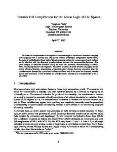
Fig. 1. (a) Condition number of the parabolic Poisson problem with periodic boundary conditions for the unpreconditioned case (solid curves) at three dierent h, and for the SGS-preconditioned (dashed curve) and ILU-preconditioned (dotted curve) cases for h,1 = 256, as a function of
t. (b) Iteration count estimates for the parabolic Poisson problem on a grid with h,1 = 64 with a convergence tolerance on the error of 10,6 in norms convenient to particular accelerator/preconditioner combinations for stationary GS, unpreconditioned CG, CG-SGS, and CG-ILU, as a function of
t.

8

usual uniform grid ve-point operator scaled to have 4 on the diagonal on a periodic square domain of n + 1 grid points on a side. Because of the periodicity, the number of cells is the same as the number of points, i.e., the mesh interval h is 1=(n + 1). We take the coordinate indices in the standard range 0  j; k  n, interpreting indices outside this range in terms of their modulus with respect to n, so that a row of Au = f becomes h2 )u , u (11) (4 +
t jk j ,1;k , uj +1;k , uj;k,1 , uj;k+1 = h2fjk : The (n + 1)2 eigenvectors are u(jks;t) = ei(js+kt ) ; 0  s; t  n; where j  j2h and k  k2h. Substituting this expression into (11), the corresponding eigenvalues are readily determined: st (A) = 4(1 + 2 ) , e,is , eis , e,it , eit = 4(1 + 2 ) , 2(cos s + cos t ) h2 + 4 , 2(cos  + cos  ) =
t s t h2 + 4(sin2 s + sin2 t ); =
t 2 2 where 2  h2 =(4
t). The largest eigenvalue is max  h2 =
t+8 at s = t   and the smallest, excluding s = 0 or t = 0, is min = h2=
t+8 sin2 (h)  h2 =
t+82h2 . The condition number is therefore 2 +8 (A)  h2 h=
t=
t + 82h2 ;

from whence it follows that lim
t!0 (A) = 1 and lim
t!1 (A)  (h),2 . Values of (A) between these saturation limits are plotted as a function of
t at h,1 = 64, 128, and 256 as the solid curves in Figure 1a. For a Dirichlet problem, the Poisson problem limit would be the classical (A)  ((h=2)),2 , justifying in this instance the claim that the periodic case condition number predicts the Dirichlet case condition number of a grid twice as coarse. To apply to the Dirichlet problem, the curves in Figure 1a should be labelled h,1 = 32, 64, and 128. Note that if
t is of the order of h2, min becomes independent of h to leading order, and all methods converge in a number of iterations independent of h. (Of course, in this case, many outer time-steps will be necessary.) If
t is of the order of h, min goes as h to leading order. Finally, if
t is large, independent of h, min behaves like h2 . In the course of the numerical results reported in Section 5 below,
t sweeps through the entire range of O(h2 ) to O(1), governed locally by nonlinear convergence criteria. In this and many other practical problems, therefore, the preferred linear solver may also vary over the course of the nonlinear trajectory. 3.3. The SGS-Preconditioned Periodic Problem. From the additive decomposition A = L + D + U and BSGS = (L + D)D,1 (U + D), we derive upon substitution of the u(jks;t) into BSGS u = (BSGS )u that st (BSGS ) = [4(1 + 2 ) , e,is , e,it ]
4(1 +1 2 )
[4(1 + 2 ) , eis , eit ] cos(s , t) : = 4(1 + 2 ) , 2(cos s + cos t ) + 1 +2(1 + 2) 9

Since BSGS and A are simultaneously diagonalized, we can easily evaluate 4(1 + 2 ) , 2(cos s + cos t) ,1=2 AB ,1=2 ) =  (B ,1 A) = st(BSGS st SGS SGS s ,t) : 4(1 + 2 ) , 2(cos s + cos t ) + 1+cos( 2(1+ 2 ) This expression can be explored analytically for its maximum and minimum in (s; t), but it is simplest for present purposes to extract the condition number by looping ,1 A over a range of
t at over all eigenpairs. A plot of the condition number of BSGS , 1 h = 256 is given as the dashed curve in Figure 1a. 3.4. The ILU-Preconditioned Periodic Problem. For a symmetric problem, we write BILU (0) as the product of a lower triangular factor, a diagonal factor, and the transpose of the lower triangular factor, and require that the elements of the product match the elements of the original where possible. Thus, A = L~ D~ ,1 L~ T , E; where E is the deviation matrix. For the constant coecient operator in question, L~ has 1's in the same o-diagonal locations as A and a to-be-determined d on the diagonal, and D~ is a diagonal matrix of all d's. Multiplying out and equating to A yields d + 2d = 4(1 + 2 ) p as the equation for d, whence d = 2[(1+ 2)+ (1 + 2 )2 , 1=2]. This leads straightforwardly to st (BILU ) = [d , e,is , e,it ]
d1
[d , eis , eit ] cos( , t) ps : = 4(1 + 2 ) , 2(cos s + cos t) + 2 (1 + ) + (1 + 2 )2 , 1=2 As above, we can easily evaluate 4(1 + 2 ) , 2(cos s + cos t ) ,1 A) = st (BILU : s ,t ) 4(1 + 2 ) , 2(cos s + cos t ) + (1+ 2 )+cos(p(1+

2 )2 ,1=2 ,1 A over a range of
t at h,1 = 256 is given A plot of the condition number of BILU as the dotted curve in Figure 1a. The condition number data of the previous three subsections is employed in (10) to generate the curves labelled \CG" in Figure 1b, which predicts iteration counts for a xed reduction in a convenient preconditioned energy norm of the error over a range of
t at a xed grid size of h,1 = 64. 3.5. Gauss-Seidel Stationary Iterations on the Periodic Problem. The curve labelled \GS" in Figure 1b is plotted from (9) on the basis of the following ,1 A)j = j(B ,1 R)j in the symmetric case for which A = derivation for j(I , BGS GS T L + D + L and BGS = D + L. ,eis , eit ,1 A) = st ((D + L),1 LT ) = st(I , BGS 4(1 + 2 ) , e,is , e,it : 10

Multiplying by the complex conjugate, 1 + cos(s , t) ,1 A)j2 = jst(I , BGS 2 2 2 8(1 + ) , 4(1 + )(cos s + cos t) + 1 + cos(s , t ) ; ,1 A) is easily found. whence (I , BGS

In comparing dierent curves in Figure 1b, it must be borne in mind that changing the method or preconditioner changes the norm in which the error is measured; thus, one should not attempt to infer in detail the cost to arrive at a particular solution, but only the trends. These plots indicate that if
t is constrained to be small by nonlinear considerations, ordinary relaxation will be competitive. 4. Test Problems. In this section, we brie y describe the ame sheet problem used to evaluate the performance of the various linear algebra solvers discussed in Section 2. The numerical solution of a ame sheet model presents a twofold interest. First, as mentioned above, ame sheet problems are on the natural route to the numerical solution of important multidimensional diusion ames. Second, the governing equations are highly nonlinear and the dependent variables are strongly coupled in the physical domain and on its boundaries so that their solution constitutes a formidable test for nonlinear elliptic solvers. The ame sheet governing equations consist of the conservation of total mass, momentum and a conserved scalar equation. The temperature and major species pro les are recovered from the conserved scalar, as described in [23]. The ow eld equations are formulated in terms of velocity and vorticity coupled together with a conserved scalar equation. As motivated in [7], a vorticity-velocity formulation allows replacement of the rst-order continuity equation with additional second-order equations. Whereas the streamfunction-vorticity formulation also accomplishes the same replacement in two dimensions, vorticity-velocity is extensible to three and allows more accurate formulation of boundary conditions in a numerically compact way. Furthermore, convective terms in o-diagonal blocks that exert a strong in uence in a streamfunction-vorticity formulation disappear. The governing equations prior to nondimensionalization are: 1 @vr + vr , @  v
r ; r2vr = @! (12) , @z r @r r2 @r  1 @vr , @  v
r ; r2vz = , @! (13) , @r r @z @z    @! + v @! , vr ! + r
r v2 , r
g; (14) r12 r
r3r ! = v r z @z r @r r 2  1 @S @S (15) r r
rDrS = vr @r + vz @z ; where v = (vr ; vz ) is the velocity vector with radial and axial components vr and vz , respectively,  the density, ! = @v@zr , @v@rz the normal component of the vorticity, g the gravity vector, 2 the viscosity, S the conserved scalar, D a diusion coecient, r2 a 2 @ @ @z r shorthand for @r2 + @z2 (not the full cylindrical Laplacian), r
(r ; z ) is @ @r + @z , @ @ and the components of r are ( @z ; , @r ). The diusion coecient D and the viscosity  depend on the temperature through a power law [23]. In our computations, typical values for the Prandtl and Reynolds numbers were 0.75 and 160, respectively. As boundary conditions on an open domain with entrainment permitted we employ along 11

the axis of symmetry (r = 0) (16) at the exit (z ! 1) (17) along the inlet (z = 0)

@S z vr = 0; @v @r = 0; ! = 0; @r = 0; @! @S z vr = 0; @v @z = 0; @z = 0; @z = 0;

r @vz 0 vr = 0; vz = vz0 ; ! = @v @z , @r ; S = S ; and along the entrainment boundary (r = R0) @vr = 0; @vz = 0; @! = 0; S = 0: (19) @r @r @r The inlet consists of an inner cylindrical fuel jet and an outer co- owing annular oxidizer jet. A schematic of this simple, extensively experimentally investigated con guration is given in Figure 2. The inlet pro le of the conserved scalar, S 0 (r), is a slightly rounded step function that blends room temperature reservoirs of fuel and oxidizer by means of a narrow Gaussian in temperature centered at RI (see Figure 2). The partial dierential equations (13){(15) together with the boundary conditions (16){(19) are discretized on a two-dimensional tensor-product grid. A solution is rst obtained on an initial coarse grid. Additional mesh points are then inserted and the coarse grid solution is interpolated onto the ner grid to yield a new solution starting estimate. A modi ed damped Newton iteration

(18)

(20)
U n = ,n J(U n ),1 F(U n); n = 0; 1; . . . with convergence tolerance k
U nk2 < 10,5, is used to solve the set of discretized equations F(U) = 0. The Jacobian is inverted at each Newton step through an inner iteration. It is important to base convergence of the linear iterative method as nearly as possible on the magnitude of k
U k2, which controls the outer Newton iteration. If our linear convergence criterion is too loose or too stringent, we may suer divergence of the outer iteration or excessive CPU time, respectively. Due to the ill-conditioning of the Jacobian, the norm of the linear residual may dier by orders of magnitude from the norm of the correction
U. In the Krylov methods, we base convergence on the norm of the left-preconditioned residual, since it scales as k
U k2 . In the SOR method, the magnitude of the update to the Newton correction is already conveniently available. All of the results presented below are obtained using an absolute linear convergence tolerance equal to one-tenth of the Newton tolerance. By this procedure, excessive CPU consumption during the pseudo-transient phase is avoided while still bringing back sucient precision in the Newton correction. To illustrate the diculties encountered when using the right-preconditioned residual as the convergence criterion, we reran selected cases with the same absolute convergence tolerance applied to the right-preconditioned residual. For instance, the coarse-grid Bi-CGSTAB/GS run required 64% more CPU time when right-preconditioned convergence was based 12

Fig. 2. Schematic of the physical con guration.

13

on the same absolute tolerance as the left-preconditioned method. The Newton convergence history was virtually unchanged. This unnecessarily stringent criterion could be partially alleviated with a mixed absolute-relative tolerance allowing termination at the earlier of the absolute criterion based on the Newton tolerance or a relative reduction of 106 in linear residual. The same test required only 33% more CPU time when based on the mixed tolerance. Due to the nonlinearity of the original problem, a pseudo-transient continuation process is used to produce a parabolic-in-time problem and bring the starting estimate on a given grid into the convergence domain of the steady Newton method. The original nonlinear elliptic problem is cast into a parabolic form by appending a pseudotransient term @U @t to the original set of algebraic equations F(U) = 0, and a fully implicit scheme solves (again with Newton's method) n+1 n (21) F (U n+1) = F(U n+1) + U
tn,+1U = 0; where
tn+1 is the (n + 1)st time step. The time step is adaptively increased as the convergence domain of the steady Newton method is approached [22] so that the solution process on a given grid may be conceived as having three main stages: an initial \deep" transient phase, a \medium" transient phase and the nal steady Newton iteration. The boundary between the rst two phases is blurred by the gradual and not necessarily monotonic buildup of
t. Typically, in driving detailed-chemistry

ame solutions towards grid-independence, an outer iteration in which the grid is adapted with respect to truncation error estimates is wrapped around each pseudotransient-to-steady-state cycle. Asymptotically, as the mesh spacing approaches zero, the interpolant of the converged solution on one grid lies in the convergence domain of Newton's method on the next ner grid [21]. 5. Numerical Results. In this section, we present several numerical experiments obtained on a Multi ow Trace 14/300 computer for the solution of the test problem described in the previous section. We compared three categories of methods for solving the linear systems arising at each Newton step: a stationary method (block-line SOR with a relaxation parameter initially set at 0.85, adjusted downward as necessary), a short-term recurrence Krylov (Bi-CGSTAB) and an optimal Krylov (GMRES). Due to memory constraints, GMRES was actually run in a non-optimal restarted mode with 20 Arnoldi vectors. The choice of 20, justi ed below, represents a balance of convergence rate and memory considerations. Both Krylov methods were combined with the three dierent left-preconditioners: block-line GS, block-line SGS, and block-point ILU. We used GS as a preconditioner rather than the somewhat more costly SOR because of our experience that relaxation methods are much less sensitive to ! as preconditioners than they are as stationary iterative methods, as also reported in [6]. In addition to varying the iterative method/preconditioner combination, we considered a coarse 41  41 and a ne 81  81 tensor-product grid. In presenting the results, we distinguish between early time steps of small size and later larger time steps in order to observe performance variations in the parabolic and elliptic limits. Coarse and ne grids adapted to the co- ow geometry are shown in Figure 3, and the converged solution for a methane-air ame sheet is shown in Figure 4. The axisymmetric ow is locally tangent to the streamfunction contours, and the mass

ux it carries in a circumferential ring is inversely proportional to the local contour spacing. The failure of the contours to close on the open outer boundary is evidence of entrainment of ambient oxidizer. In engineering practice, the outer boundary con14

Fig. 3. The grids: (a) a coarse grid, showing concentration of mesh lines in the high activity regions

of the ow domain, and (b) a self-similar ne grid.

15

dition of a zero gradient on the vorticity may be replaced with its de nition in terms of the velocity derivatives, which we have observed to yield less entrainment of uid across the outer boundary. The temperature eld plot in Figure 4b, obtained from the solution for the conserved scalar S as described in [23], varies from an ambient temperature of 298 K to approximately 2000K in a distance of millimeters. Interpretative discussions of similar results for ame sheet, reduced kinetics, and full kinetics

ame models may also be found in [23, 26] and references therein. 5.1. General Comparisons. The algorithmic performance results obtained on the coarse 41  41 grid are summarized in Table 1. We found that a minimum of 850 adaptively increased time steps had to be taken in order to bring the initial estimate into the convergence domain of the steady Newton method. The initial time step was set at 10,8 and was allowed to increase adaptively [22]. By the time a switchover to the steady-state form of the equations could be undertaken,
t had typically reached O(1). The rst line of Table 1 presents the memory requirement in double precision words for each method. The extra overhead of the Krylov space is re ected in the GMRES columns, and it is seen that the use of an ILU preconditioner approximately doubles the storage requirement with respect to the standard relaxation method. The second line shows the CPU time needed per inner linear iteration averaged along the pseudo-transient iterations; these numbers are normalized by the corresponding SOR time in line 3. The lines four to six show the total amount of CPU time spent on the linear algebra solves for the rst 5, 10 and 20 time steps, respectively. At this stage of the transient iteration, the time step is small so that a relaxation method is quite competitive with a Krylov method preconditioned with Gauss-Seidel whereas the use of other preconditioners (SGS or ILU) tends to be more expensive. It is clear from the last three lines of Table 1, representing the total CPU time spent on the pseudo-unsteady iteration, the steady Newton method, and the whole algorithm, respectively, that the best overall results are obtained by combining either Bi-CGSTAB or GMRES(20) with the Gauss-Seidel preconditioner and, from a storage point of view, the former algorithm is preferable. Relaxation methods meet with diculty when the time step is increased and are ineective in the fully elliptic phase of the iteration. The asterisks in the SOR column indicate that linear convergence on the steady-state system was eventually achieved with a relaxation factor ! of 0.3, instead of the previously sucient 0.85. The combination of GMRES(20) with SGS stagnates due to loss of orthogonality in the Krylov vectors. The use of an ILU preconditioner is not very attractive for these problems because, in the coarse grid case, most of the CPU time is spent in the pseudo-transient continuation process to bring the iterate into the convergence domain of the steady Newton method. The decrease of inner iterations needed to invert the Jacobian matrix with either the SGS or ILU preconditioners is not sucient to compensate for their higher cost per iteration. This results in an increase of the overall CPU time by a factor of 1.4 and 2.1 for SGS and ILU, respectively. Finally, the use of ILU preconditioning nearly doubles the memory requirements in problems already dominated by Jacobian storage. In detailed chemistry combustion models, where the dominant term in the storage, due to the Jacobian, scales like n2c , available memory limits the choice of nc, which may be as high as 40 in current practice [23]. We discuss next the results obtained on the ner 81  81 tensor-product grid. Although the interpolated coarse grid solution lay in the domain of convergence of the steady Newton method on the ner grid, we found it more ecient overall to take several time steps before starting the steady Newton iteration. After time steps are 16

Fig. 4. The converged solution: (a) variable-density Stokes streamfunction, and (b) temperature. Table 1

Performance results on the coarse grid.

Algorithm Preconditioner work array (Mw) time/it (min) 10,3 time/SOR-time time/5 steps (min) time/10 steps (min) time/20 steps (min) time/transient (min) time/steady (min) Total time (min)

SOR { 0.31 2.83 1.0 0.13 0.25 0.48 156 94 250

Bi-CGSTAB GS SGS ILU 0.35 0.35 0.60 6.56 16.6 26.6 2.3 5.9 9.4 0.09 0.21 0.33 0.20 0.40 0.62 0.42 0.78 1.22 121 162 246 9 18 24 130 180 270 17

GMRES(20) GS SGS ILU 0.45 0.46 0.70 4.27 11.7 20.7 1.5 4.1 7.3 0.09 0.18 0.32 0.18 0.35 0.62 0.36 0.73 1.20 117 154 243 9 { 28 126 { 271

taken, the Jacobian matrices at the rst and second Newton steps are less expensive to invert so that an optimal balance exists between the CPU time spent in the parabolic and elliptic phases. In our computations, 10 time steps between 10,6 and 10,5 represented an excellent compromise. Numerical results are summarized in Table 2 using the same notation as in Table 1. Once again, the shortest overall execution time is obtained by using a Krylov method preconditioned with GS, and a short-term recurrence may be then preferable rather than an optimal method from a storage point of view. The relaxation method compares very favorably during the deep transient steps but is unable to solve the elliptic linear systems with the original relaxation factor of 0.85. The asterisked execution times were obtained with a reduced factor of 0.65. With intermediate values of 0.75 and 0.70 for !, SOR was able to take only the rst steady Newton step and the rst two steady Newton steps, respectively. As in the coarse grid case, the use of either SGS or ILU preconditioning does not present any advantage and it is interesting to note that GMRES(20)/ILU even stagnates as opposed to the much simpler GS and SGS preconditioners. The convergence history of all the above Krylov methods is illustrated in Figure 5 for both grid cases by representing the residual norm versus CPU time during the inner iterations for the rst steady Newton step. The characteristic staircase pattern of restarted GMRES and the highly nonmonotonic convergence history of Bi-CGSTAB are evident. We have observed above that 20 Krylov vectors are not sucient to prevent GMRES from stagnating in certain steady Newton cases. Our uniform choice of 20 vectors in the reported results stems from numerical experiments with as few as 5 and as many as 30 vectors, using the GS preconditioning. With Krylov spaces of dimensions 5 and 10, even the coarse grid problems stagnated. The same diculty was encountered on the ne grid with dimension 15. In the other limit, allowing as many as 30 vectors led to fewer restart cycles during the steady Newton iteration with overall CPU savings of 26% and 2% on ne and coarse grids respectively, but at a cost of approximately 15% more in storage. It therefore appears that special care should be taken in selecting the Krylov dimension in order to avoid both stagnation in the steady Newton iteration and excessive storage requirements in the pseudo-transient stage. Following a suggestion of Van der Vorst, we reran the Bi-CGSTAB/GS cases ,1 A)T r0 in order to attempt to observe on both coarse and ne grids with r~0 = (BGS a decrease in iterations often associated with this practice. We found decreases in iterations relative to r~0 = r0 in the steady-state Newton iteration for both coarse and ne grids, the savings in CPU time being as high as 18%. In contrast, the convergence improvements were marginal and the execution times greater when this device was employed in the pseudo-transient phase. The associated CPU time penalty was as high as 18%. This is mainly attributable to the extra cost of forming and factoring a second set of diagonal blocks of the Jacobian for use in the application of the transpose of the preconditioner. Their cost is not amortized over many subsequent iterations since the pseudo-transient linear systems converge fairly rapidly. We should also mention that the use of the exible variant of GMRES, namely FGMRES [18], preconditioned alternatively by lower and upper triangles, did not meet with success. In fact, the alternate use of these two preconditioners seemed to uncondition the system for this test problem and the results were much worse than with a lower triangle preconditioner (GS) alone. Finally, we point out that for ame sheet problems the cost of evaluating the Jacobian does not represent a signi cant number of linear iterations and the best overall strategy for these problems is to 18

Fig. 5. Plots of preconditioned residual norm as a function of execution time for Bi-CGSTAB and GMRES(20) using each of three preconditioners on coarse and ne grids for the rst steady Newton step (
t = 1).

19

Table 2

Performance results on the ne grid.

Algorithm SOR Bi-CGSTAB Preconditioner { GS SGS ILU work array (Mw) 1.22 1.35 1.38 2.32 , 2 time/it (min) 10 1.17 2.88 6.47 10.6 time/SOR-time 1.0 2.5 5.5 9.1 time/5 steps (min) 1.04 0.93 1.63 2.05 time/10 it (min) 1.83 1.64 2.92 3.63 time/transient (min) 4.1 3.5 5.0 8.3 time/steady (min) 104.9 25.0 49.1 59.3 Total time (min) 109.0 28.5 54.1 67.6

GMRES(20) GS SGS ILU 1.77 1.80 2.74 1.70 5.25 8.38 1.5 4.5 7.2 0.84 1.78 1.96 1.46 3.40 3.53 3.5 5.8 8.3 26.3 48.6 { 29.8 54.4 {

Table 3

Performance of Bi-CGSTAB/GS and GMRES/GS by grid and time-stepping phases.

Problem Bi-CGSTAB/GS GMRES/GS Coarse Grid Newton its. 1,662 1,664 Transient Krylov its. 12,550 19,661 time (min) 120.5 116.7 Coarse Grid Newton its. 7 7 Steady Krylov its. 1,595 2,724 time (min) 9.4 9.2 Fine Grid Newton its. 14 14 Transient Krylov its. 57 86 time (min) 3.5 3.5 Fine Grid Newton its. 4 4 Steady Krylov its. 1,102 2,006 time (min) 25.0 26.3 Total Newton its. 1,687 1,689 Krylov its. 15,304 24,477 time (min) 158.4 155.7 re-evaluate the Jacobian at each time step. For instance, in the ne grid case, the evaluation of the Jacobian takes as much time as 4.7 Bi-CGSTAB/GS iterations. Consequently, the savings on Jacobian evaluations from keeping the Jacobian xed for several time steps does not compensate for the resulting increase in the number of linear iterations. This contrasts with our experience in larger combustion systems, such as a 29-species methane-air ame, in which a Jacobian evaluation costs the equivalent of 14 Bi-CGSTAB iterations, so that it is preferable to keep it xed for several time steps, especially during the initial deep transient phase. 5.2. Detailed Comparisons of Bi-CGSTAB/GS and GMRES/GS. According to the results of the previous section, the two most eective algorithms over the course of the entire solution history are Bi-CGSTAB/GS and GMRES(20)/GS. These algorithms never fail to converge and deliver total CPU times that are within 2% of each other on the two dierent grids. Bi-CGSTAB accomplishes this with approximately 30% less memory than does GMRES(20). 20

Table 3 breaks down the counts of Newton steps and Krylov iterations and the CPU time over each of four easily demarcated phases of the overall two-grid computation. As summarized in the left-most columns, these phases consist of: 850 adaptively chosen transient Newton steps on a coarse grid of 40 subintervals on each side, followed by a steady Newton iteration on the same grid, followed by interpolation onto a grid formed by doubling the re nement in each coordinate direction and 10 adaptively chosen time steps on this new grid, followed by a steady-state iteration on the ne grid. The count of Newton iterations includes all of the correction vectors
U that are accepted by the algorithm, sometimes after damping. (Because of the control structure of the nonlinear algorithm, this is not the same thing as the total number of linear systems (20) of size nc
nr
nz solved. Many of these Newton corrections are provisional \look ahead" vectors that are ultimately discarded.) The counts of preconditioned Krylov iterations (of either Bi-CGSTAB or GMRES type) are the totals over all calls to the linear solver. This is the same as the number of calls to the subroutine that evaluates matrix-vector products for GMRES; for Bi-CGSTAB, the matrix-vector subroutine is called twice in each iteration. Likewise, the subroutine that evaluates vector inner products is called four times for each tabulated Bi-CGSTAB iteration. It is not possible directly to infer the number of inner products from number of GMRES iterations because of the ever expanding space of direction vectors against which GMRES orthogonalizes each iterate. However, each full restart cycle of 20 Krylov vectors requires 20  21=2 = 210 inner products, so we can upper bound the number of inner products per GMRES iteration at 10.5. It would appear that the nonlinear convergence history is independent of the linear solver, since the total number of Newton steps is nearly identical. In fact, a detailed iteration-by-iteration comparison reveals this not quite to be the case. The convergence tolerance for the Krylov methods is loose enough to allow slightly dierently shaped correction vectors (whose linear residuals satisfy the same Euclidean bound) to be returned to the Newton method. Appreciable discrepancies (on the order of a factor of 2) in nonlinear residual norm between the Bi-CGSTAB and GMRESdriven solvers occur only in the last few Newton iterations, after the norm has dropped a million-fold. However, the number of Newton iterations to complete convergence is not aected. In the transient portions of the solution trajectory, when the diagonal dominance of the Jacobian is enhanced by the time-stepping, the number of Krylov vectors required per Newton step is one to two orders of magnitude less than the number required during the steady-state portions, for both Bi-CGSTAB and for GMRES. In the transient ne-grid computation, for instance, Bi-CGSTAB requires approximately 4.1 iterations per Newton step, and GMRES approximately 6.1. On the other hand, in the steady coarse-grid computation, Bi-CGSTAB requires approximately 276 iterations per Newton step, and GMRES approximately 502. (Because \look-ahead" steps are frequently discarded during the steady Newton stage of the computation, the average numbers of Bi-CGSTAB and GMRES iterations per linear system solved are closer to half these totals.) For a xed state of the physical system, the Jacobian constructed on the ne grid is more dominated by the elliptic, second-derivative terms of (13){(15) than by the rst-derivative terms. The tables do not contain a control experiment in which the identical physical state is discretized on each of the two grids, but we can observe that Bi-CGSTAB is on average equal to or slightly better than GMRES in terms of CPU time on the ne grid, whereas GMRES is slightly better than Bi-CGSTAB on 21

the coarse grid. Comparing the iteration counts of Bi-CGSTAB and GMRES, we see that the former is 62.5% of the latter, averaged over a complete computation, ranging from about 55% to about 66% for dierent phases of the computation. This translates into the Bi-CGSTAB solver making 25% more matrix-vector product calls than GMRES. On the other hand, over a complete calculation, GMRES makes just under 3 times as many calls to the inner product routine as Bi-CGSTAB. Given the readily apparent dierences between the distribution of work of the two linear solvers, it is interesting that their CPU times match very closely within each phase. 6. A Multidomain Preconditioner. In this section, we reexamine the blockline Gauss-Seidel preconditioner with a view toward parallelism. Computational combustion is driven in this direction by both memory requirements and execution time requirements, even for two-dimensional problems. As is widely appreciated, NewtonKrylov methods for nite-dierence discretizations are easily and eciently parallelized by domain decomposition, except, possibly, for two tasks: inner products and preconditioning steps with internal sequentiality or extensive non-local data dependencies. Apart from these tasks, Newton-Krylov solvers consist mainly of residual evaluations, Jacobian evaluations, and sparse matrix-vector products, in which the worst data dependencies can be con ned to nearest-neighbor type. Inner products of distributed vectors involve global synchronized communication. Possibilities for recasting Krylov algorithms to form several inner products simultaneously within a vector global reduction operation have been explored by many authors with views towards stability and computational complexity, and are beyond the scope of this article. However, the sequentiality of the block-line Gauss-Seidel preconditioner has been addressed through the following simple modi cation. ,1 Ax is still formed in two steps as in Section The preconditioned product y = BGS 2.1.1, but for multidomain Gauss-Seidel (GS) we replace L with an L^ in the factor to be inverted: solve (L^ + D)z = Ux + (L , L^ )x; y z + x. The operator L^ is just L with the o-diagonal row blocks that contain the coupling of each subdomain to the one upstream set to zero. In our application, a subdomain consists of a collection of contiguous rows of gridpoints oriented normal to the predominant ow direction. For the case of two subdomains on the coarse grid, for instance, the downstream subdomain spanning rows j = 22 through j = 41 takes its upstream data at iteration k from the data along row j = 21 after iteration k , 1. We have previously experimented with a similar \poor man's" type of domain decomposition preconditioner in the context of block-ILU subdomain preconditioners in [14]. Though its eectiveness does not scale to the ne parallel granularity limit in elliptic systems, it is a simple and practical device at coarse granularity, motivated by the following elementary observation. Let A be a banded matrix, written in block 2  2 form (22)

A = [ A11 A12 A21 A22 ]:

The A11 block corresponds to subdomain 1 and A22 to subdomain 2, with coupling blocks A12 nonzero only in its lower left corner and A21 only in its upper right. Let B be a conformally blocked diagonal preconditioner  ,1  B = A011 A0,1 : (23) 22 22

Table 4

Performance of the multidomain preconditioner with Bi-CGSTAB (timings in minutes).

Problem 1 Domain 2 Domains 4 Domains 8 Domains 8:1 Ratios Coarse Grid Transient 120.5 122.2 121.6 126.7 1.05 Coarse Grid Steady 9.4 10.1 9.7 11.0 1.17 Fine Grid Transient 3.5 3.5 3.5 3.5 1.00 Fine Grid Steady 25.0 28.0 29.2 27.5 1.10 Total 158.4 163.8 164.0 168.7 1.07 Table 5

Performance of the multidomain preconditioner with GMRES(20) (timings in minutes).

Problem 1 Domain 2 Domains 4 Domains 8 Domains 8:1 Ratios Coarse Grid Transient 116.7 121.1 118.2 123.0 1.05 Coarse Grid Steady 9.2 9.3 9.7 11.0 1.19 Fine Grid Transient 3.5 3.5 3.5 3.5 1.00 Fine Grid Steady 26.3 23.5 23.3 22.8 0.87 Total 155.7 157.4 154.7 160.3 1.03 The preconditioned operator is





I A,111 A12  I + R: (24) , 1 A22 A21 I In the context of a naturally ordered two-dimensional PDE discretization with O(n) mesh intervals on a side, the dimension of B ,1 A is O(n2 ) and the rank of R is O(n). Hence conjugate gradients on a symmetrizable B ,1 A will converge in at most O(n) iterations [11], which is acceptable relative to other comparably parallelizable methods as n becomes large. Tables 4 and 5 display the results of rerunning the Bi-CGSTAB and GMRES(20) tests with the modi ed preconditioner. The rst columns show the same timing data as in Table 3. The next three columns display the results of complete computations carried out on the same serial machine as the single domain computation. At the maximum granularity of 8 subdomains, the line Gauss-Seidel preconditioning is commenced independently in each of 8 strips that are, respectively, 5 and 10 grid cells wide in the streamwise direction on the coarse and ne grids. As can be observed from the ratios in the nal column, comparing the cases of 1 and 8 subdomains, the penalty in CPU time paid by this modi cation is very modest: 7% under Bi-CGSTAB and only 3% under GMRES. It has become conventional in reporting parallel eciencies to distinguish between the \numerical eciency," num , of a multithreaded algorithm relative to the best single-threaded algorithm and the \machine eciency," mach, of the multiprocessor implementation of the multithreaded algorithm. In this nomenclature, the nal column lists the reciprocals of the numerical eciency of the parallelized preconditioning. We conclude that modest granularity parallel preconditioners are available for these problems at a very small price in terms of convergence degradation relative to an excellent serial preconditioner. It is perhaps surprising that there are a few non-monotonicities in the convergence behavior of both linear solvers as the number of severed j-lines increases. Moreover, on the ne grid during the nal steady Newton iterations, the convergence of GMRES B ,1 A =

23

is actually monotonic in the unexpected direction for the rst three mesh bisections shown. However, GMRES(20) stagnates when the preconditioner is further decoupled into 16 subdomains. We do not fully understand the circumstances under which using data that is less than the best available (i.e., moving away from Gauss-Seidel towards Jacobi) will enhance convergence, but we can oer the following observations concerning the plausibility of encountering such behavior:  First, this problem is multicomponent. In some regions of the ow eld, the strongest couplings of one degree of freedom to all others occur not between unknowns of the same type at neighboring points in space, but between unknowns of dierent type (e.g., velocity and vorticity) at the same point in space. Furthermore, in pseudo-transient phases with very small time step, the strongest coupling of each degree of freedom is to its own image at the previous time step. Therefore, weakening spatial dependencies does not always make a leading-order dierence in the update formula for a given degree of freedom.  Second, the linear operators are not symmetric positive de nite; recall that SOR used as a stationary iteration actually requires under-relaxation for convergence throughout the entire solution trajectory. The modi cation of Gauss-Seidel described above is a form of under-relaxation.  Third, we do not iterate to machine precision within each linear solution process; therefore, there is an interaction between the linear and nonlinear residuals. When the preconditioner changes, the shape of the incompletely converged Newton correction changes, which results in a dierent Jacobian matrix and right-hand side vector at the next Newton step. Our numerical experiments show that for ner granularity preconditioners more inner iterations are needed to solve the rst steady Newton step; on the other hand, further nonlinear progress is made in the sense that the norm of the nonlinear residual is further reduced by the resulting step. The next Newton step then generally requires fewer linear iterations for its computation. The result is an oscillation in the linear iteration history for the decoupled problems around the linear iteration history for the single-domain problems. Threshhold eects of this oscillation along the course of the steady nonlinear iterations account for the variations in cumulative linear iterations as the number of subdomains is increased. 7. Conclusions. In this study, we compared a standard relaxation method and two CG-like algorithms combined with three preconditioner options in the solution of linear systems arising in axisymmetric ame sheet simulation problems. Both traditional (SOR) and recent (Bi-CGSTAB) solvers occupy practical niches. Though SOR cannot handle the Jacobians of the steady Newton steps on the coarse grid as early as the Krylov methods in the present problem, it has been successfully employed in streamfunction-vorticity [23], primitive variable [26], and vorticity-velocity [7] formulations both with and without chemical reaction by prolonging the pseudo-transient stage and by under-relaxation. By handling fully implicitly the intra-point coupling, block-SOR can be regarded as the most economical splitting matrix for problems in which the dominant coupling is through the source terms or backwards to the previous iterate through the implicit time-dierencing. The Bi-CGSTAB algorithm combined with a Gauss-Seidel left-preconditioner gives the best execution time and does not break down in our experience. Bi-CGSTAB/GS permits passage to steady Newton iteration at an earlier stage than SOR. GMRES/GS yields nearly identical execution 24

times without concern for breakdowns, but at a higher storage overhead in problems in which memory may be a premium. With an eye towards future applications, it should be noted that either BiCGSTAB or GMRES can be employed as inner iterative loops of Newton's method in matrix-free variants with preconditioners that might rely on evaluation and storage of only selected portions of the Jacobian, or only infrequent evaluation of the Jacobian. It is to preserve this possibility on problems with more expensive Jacobian evaluations that we avoid linear solvers with an explicit reliance on matrix-vector products with the transpose of the Jacobian. For coarse-granularity parallel computation in which each processor is responsible for a dierent subdomain, we have demonstrated that a number of the o-diagonal blocks of the Gauss-Seidel preconditioner coupling adjacent subdomains may be discarded with minor penalty, leaving a block-Jacobi-like structure to the outermost iteration. This approach has been implemented in [15] and in [20]. In the latter fullscale implementation of a 26-species, 78-step reaction mechanism for a methane-air

ame, an overall eciency of 82% is reported on a six-processor IBM ES/3090 600J. Gauss-Seidel still retains its usefulness as a subdomain preconditioner. For ner granularity parallelism, we would expect to combine it into a global preconditioner based on hierarchically coarsened grids. Simple, two-level hierarchies have been extensively tested under the rubric of \domain decomposition" methods. For some parallel performance results on model two-dimensional problems with convection and adaptive re nement, see [12]. Finally, on ne-grained distributed parallel architectures with dierential rates for communicationinvolving local and global data dependencies, the trade-o between the generally greater number of matrix-vector products in Bi-CGSTAB and the generally greater number of inner products in GMRES may play a more signi cant role than CPU and total storage considerations in selecting among linear solvers. REFERENCES [1] G. Bader and E. Gehrke, Solution of ame sheet problems on transputer networks, in Flow Simulation on Supercomputers, Notes on Numerical Fluid Mechanics, Vol. 38, E. H. Hirschel, ed., Vieweg Verlag, 1993. [2] T. F. Chan, Fourier analysis of relaxed incomplete factorization preconditioners, SIAM Journal of Scienti c and Statistical Computing, 12 (1991), pp. 668{680. [3] T. F. Chan and H. C. Elman, Fourier analysis of iterative methods for elliptic boundary value problems, SIAM Review, 31 (1989), pp. 20{49. [4] T. F. Chan, C.-C. J. Kuo, and C. Tong, Parallel elliptic preconditioners: Fourier analysis and performance on the connection machine, Computer Physics Communications, 53 (1989), pp. 237{252. [5] H. A. V. der Vorst and C. Vuik, GMRESR: A family of nested GMRES methods, Tech. Rep. 91-80, Technological University of Delft, 1991. [6] A. Ecder, Krylov Methods in Transport Modeling, PhD thesis, Yale University, May 1992. [7] A. Ern and M. D. Smooke, Velocity-vorticity formulation for three-dimensional steady compressible ows, Journal of Computational Physics, 72 (1993), pp. 58{71. [8] V. Faber and T. A. Manteuffel, Necessary and sucient conditions for the existence of a conjugate gradient method, SIAM Journal of Numerical Analysis, 21 (1984), pp. 352{362. [9] R. W. Freund, A transpose-free quasi-minimum residual method for non-Hermitian linear systems, Tech. Rep. 91.18, RIACS, NASA Ames Research Center, 1991. [10] R. W. Freund and N. M. Nachtigal, QMR: a quasi-minimal residual method for nonHermitian linear systems, Numerische Mathematik, 60 (1991), pp. 315{339. [11] G. H. Golub and C. F. V. Loan, Matrix Computations, Johns Hopkins, Johns Hopkins, Baltimore, 1989. 25

[12] W. D. Gropp and D. E. Keyes, Parallel performance of domain-decomposed preconditioned Krylov methods for PDEs with locally uniform re nement, SIAM Journal of Scienti c and Statistical Computing, 13 (1992), pp. 128{145. [13] I. Gustafsson, Modi ed incomplete cholesky (MIC) methods, in Preconditioning Methods: Analysis and Applications, D. J. Evans, ed., New York, 1983, Gordon and Breach. [14] D. E. Keyes, Domain decomposition methods for the parallel computation of reacting ows, Computer Physics Communications, 53 (1989), pp. 181{200. [15] D. E. Keyes and M. D. Smooke, Flame sheet starting estimates for counter ow diusion

ame problems, Journal of Computational Physics, 72 (1987), pp. 267{288. [16] N. M. Nachtigal, S. C. Reddy, and L. N. Trefethen, How fast are nonsymmetric matrix iterations?, SIAM Journal of Matrix Analysis and Applications, 13 (1992), pp. 778{795. [17] E. S. Oran and J. P. Boris, Numerical Simulation of Reactive Flow, Elsevier, New York, 1987. [18] Y. Saad, A exible inner-outer preconditioned GMRES algorithm, Tech. Rep. 91/279, University of Minnesota Supercomputer Institute, 1991. [19] Y. Saad and M. H. Schultz, GMRES: A generalized minimal residual algorithm for solving nonsymmetric linear systems, SIAM Journal of Scienti c and Statistical Computing, 7 (1986), pp. 856{869. [20] M. D. Smooke and V. Giovangigli, Numerical modeling of axisymmetric laminar diusion

ames, Impact of Computing in Science and Engineering, 4 (1992), pp. 46{79. [21] M. D. Smooke and R. M. M. Mattheij, On the solution of nonlinear two-point boundary value problems on successively re ned grids, Applied Numerical Mathematics, 1 (1985), pp. 463{488. [22] M. D. Smooke, J. A. Miller, and R. J. Kee, Solution of premixed and counter ow diusion

ame problems by adaptive boundary value methods, in Numerial Boundary Value ODEs, New York, 1985, Birkhauser. [23] M. D. Smooke, R. E. Mitchell, and D. E. Keyes, Numerical solution of two-dimensional axisymmetric laminar diusion ames, Combust. Sci. and Tech., 67 (1989), pp. 85{122. [24] P. Sonneveld, Cgs, a fast lanczos-type solver for nonsymmetric linear systems, SIAM Journal of Scienti c and Statistical Computing, 10 (1989), pp. 36{52. [25] H. A. Van der Vorst, Bi-CGSTAB: a more smoothly converging variant of CG-S for the solution of nonsymmetric linear systems, SIAM Journal of Scienti c and Statistical Computing, 13 (1992), pp. 631{644. [26] Y. N. Xu, Numerical Calculations of an Axisymmetric Laminar Diusion Flame with Detailed and Reduced Reaction Mechanisms, PhD thesis, Yale University, May 1991.

26