Towards Quality-aware Simulations on Mobile Devices - Informatik.uni ...

Towards Quality-aware Simulations on Mobile Devices Christoph Dibak, Boris Koldehofe Institute for Parallel and Distributed Systems University of Stuttgart Universitätsstraße 38 70569 Stuttgart, Germany {firstname.lastname}@ipvs.uni-stuttgart.de Abstract: Numerical simulations are import for analyzing Big Data and realizing applications in the Internet of Things. Running numerical simulations on mobile devices makes analyzing and reasoning about Big Data ubiquitous. However, mobile devices are limited in energy and compute resources, and connectivity to a dedicated infrastructure like a cloud cannot always be assured. Therefore, we propose to run the simulation on a distributed environment consisting of a mobile device and the cloud. This environment has a number of constraints for compute and network resources that need to be considered for providing simulation results in time and with high quality. In this paper we propose an architecture for mobile simulations and list challenges for realizing them.

1

Introduction

Numerical simulations have many applications ranging from stress tests in computer aided designs (CAD) over traffic analysis to weather forecast. In engineering and natural sciences, dynamic complex systems and processes are often described by means of partial differential equations. Numerical simulations allow understanding the dynamic evolution of such systems that follow from such a description. Numerical simulations are also important for analyzing huge data sets in the context of Big Data and the Internet of Things. Given real-world measurements and data, simulations can predict important future critical states or situations within a complex system. Embedded in a control-loop, a controller can react to predicted states in order to optimize or stabilize the future evolution of the system. Whenever the result of a simulation needs to be directly available on a mobile device, the term mobile simulation can be applied. For instance, a controller reacting to critical states and situations in traffic, navigation, or logistics is embedded in a car, ship or drone. Furthermore, in a wide range of applications like medicine, sports, or agriculture, decision makers like the doctor, trainer, or farmer require personalized simulations that depend on the current context, e.g. the status of a patient, the training activity, or plants. A key challenge is how to realize mobile simulations so they yield i) sufficient quality of result, ii) offer the actors sufficient responsiveness and iii) are energy efficient for the mobile device. Naive methods in deploying mobile applications are likely to yield unsatisfactory

Published in 44. Jahrestagung der Gesellschaft für Informatik e.V. (GI) (Informatik 2014) LNI, 2014. © Gesellschaft für Informatik, Bonn, 2014 The original publication will be available at Lecture Notes in Informatics (LNI): http://www.gi.de/service/publikationen/lni/

results in the context of mobile simulations. First, mobile simulation may be executed similar to traditional simulations on a high performance computing infrastructure, offered by a cloud provider. Although a simulation may benefit from strong compute resources, temporal loss of connectivity is common in mobile services and can severely impact the time until actors can react to simulated results, e.g. when no network is available. Second, loss of communication may be tackled by running the entire simulation on the mobile device themselves. Even though mobile devices are becoming more powerful and already replace their stationary counterparts in many fields like image and video processing, it should be observed that simulations are highly demanding regarding processing resources. Simulations like in fluid dynamics require solving linear equations with thousands of unknowns. Performing all computations of a simulation on the mobile device will therefore lead to high response time and energy usage or allow only low quality results by simplifying the underlying simulation model. In this paper, we present our vision towards supporting mobile simulations that establishes a trade-off between the two deployment possibilities dynamically under run-time constraints like the connectivity of the mobile and constraints of the decision maker on time and quality to respond to results of a simulation. In the remainder of the paper we give an overview of what numerical simulations are and how mobile simulations can be realized using existing work. In Section 3 we propose an architecture to realize mobile simulations overcoming the drawbacks from a naive deployment. Section 4 describes challenges for implementing this architecture, possible methods and further aspects to be regarded during implementation of the proposed architecture.

2

Background

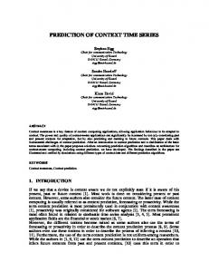
In numerical simulations, the behavior of the system is described by a mathematical model such as partial differential equations (PDEs). These equations are defined on continuous space and time also called domain of the simulation. As computers are not capable of dealing with continuity, time and space need to be mapped to a finite set of discrete points. The discrete points form a mesh on the continuous spaces. Using this mesh, the partial differential equations can be numerically solved using a system of linear equations. Figure 1 gives an overview of the process. On the left, the numerical treatment of PDEs is depicted. The model is kept in partial differential equations. These PDEs are discretized using techniques such as finite elements, finite differences or finite volumes. Those discretization techniques allow transforming the simulation to a finite mathematical problem like linear equations. The mathematical problem is then solved using a task-specific Solver, e.g. to solve a system of linear equations iteratively. In this paper, we deal with the question how to run this process within a distributed environment consisting of the mobile device and a server hosted in the cloud (cf. right side of Figure 1). In order to run the numerical simulation on this environment, quality has to be adapted to run-time constraints of the user and the available network and compute resources. There are a number of methods of how mobile simulations could be realized using existing

Mobile Device

PDE

Distributed Execution

Discretization Techniques Solver

Methods to adopt Quality

Cloud

Figure 1: Numerical simulations have to be adopted to run-time constraints in order to run on a mobile distributed environment.

work which can be categorized into two main classes. On the one hand, there are methods reducing quality of simulation so that the entire simulation can be efficiently executed on the mobile device [ASG01,HDO11]. On the other hand, there are methods to execute programs on a distributed infrastructure [CBC+ 10, CIM+ 11, RSM+ 11, GRA12, Fuj99, BPOS12]. In model reduction, the numerical simulation is transferred into a lower dimensional space [ASG01, HDO11]. This reduces quality, while it also reduces computational cost. Using model reduction, it is possible to run the entire simulation on mobile devices. A drawback of the approach is that no additional compute resources accessible over a wireless link can be used. Utilizing many compute resources in the course of a simulation is often addressed in high performance computing by a parallelization of the simulation’s execution [Fuj99, BPOS12]. However, the execution of a parallel simulation requires very frequent exchanges of states and synchronization between the parallel simulation instances. Therefore, parallelization yields good response time only when—unlike in a mobile environment—communication is subject to low latencies and high availability. A promising alternative are code offloading techniques. Code offloading is a paradigm where some parts of a mobile computation is offloaded to the cloud in order to either speed up the application [RSM+ 11,GRA12] or to save energy on the mobile device [CBC+ 10,CIM+ 11]. While both aspects are important for mobile simulations, code offloading is oblivious to the quality of the results of an application. In particular, code offloading per se will not be able to benefit from different discretization parameters of the simulation model.

3

An Architecture for Mobile Simulations

The proposed architecture of the mobile simulation middleware supports the execution of a mobile simulation to be executed on two interconnected nodes, the mobile device and a server in the cloud. Both nodes are assumed to be connected through a wireless communication link such as WiFi (IEEE 802.11) or a cellular network. As the mobile device is carried by users, the wireless connection is subject to varying bandwidth, e.g. a mobile device might leave the coverage area of its company’s WiFi and therefore has to

rely on cellular networks, providing significant lower bandwidth. In order to initiate a simulation a request needs to be posed to the middleware in form of a tuple (tS , tD ). The request defines that state of the simulated system at time tS should be available on the mobile device before the deadline tD expires. Our middleware should provide an adequate quality with respect to a trade-off between available resources and risk to exceed the deadline tD . Note, there is no perfect simulation. As it would cost too much compute resources to simulate all effects, some aspects of the real-world system have to be omitted during modeling and implementation [BZBP09]. In order to make run-time decisions our middleware requires to change some well-defined parameters during run-time that effect the trade-off between computation cost and quality. This may include time and space discretization grids (cf. Section 2). There are further parameters, e.g. the maximum error of an iterative solver after the discretization process or even different models for simulating the system. However, we will focus on discretization grids as they have a significant impact on computation time and state transfer volume. The method of how quality can be adopted in the discretization process depends on the applied discretization method. For finite differences, only the mesh size can be changed. For more advanced discretization techniques like finite elements, test functions can also be changed [BZBP09]. However, as the method used for discretization is chosen by the programmer, she also has to specify how quality can be changed in her implementation. Figure 2 depicts our architecture consisting of four components, named discretization controller, quality predictor, resource statistics and run-time protocol. These components will be explained in detail in the remainder of this section in the context of the following example: Consider a sailor on a boat near the cost and the sailor wants to find the fastest route to a nearby harbor. The fastest route depends on the wind flow near the coast. Wind depends on weather conditions as well as the structure of the coast like hills. To keep our simulation simple, we will neglect the flow of the sea and just focus on the wind flow. The behavior of wind flow will be modeled using Navier-Stokes equations [KPL00]. In our example, these equations are discretized using the finite volume method. For simplicity, we assume a quadratic 2D spatial domain. The quadratic domain is cut into squares of width Δx. The time domain is divided into equidistant time steps of length Δt. The simulation will provide the sailor with a map of the wind flow. This map is generated using data of nearby weather stations. In a more advanced example, sensor data of nearby boats might also be integrated into the simulation. To run and see the results of the mobile simulation, the sailor uses a mobile device like a tablet or smartphone. Dependent on the distance to the coast the communication link between the mobile device and the cloud can strongly vary in its characteristics. If the sailor is near the coast, the device might be connected through a 3/4G cellular network. When the sailor is too far off the coast, the mobile device may require satellite communication, or there may be temporarily no connection at all.

User Query ( , )

Middleware dl

Quality Predictor Discretization Controller

Runtime Protocol

Resource atistics Statistics

Mobile Device Link

Simulation Data

Simulation Model

Cloud Runtime Constraints

Figure 2: Components of the Architecture for Mobile Simulations

3.1

Quality Predictor

For multiple discretization parameters it is hard to find the optimal combination in order to have good quality with low computational cost. The question whether further compute resources should be invested for having finer spatial (in our example Δx) or finer temporal (in our example Δt) discretization to achieve maximum quality is not trivial [LDBNR13]. The quality predictor component is used to predict the quality of a fixed combination of discretization parameters. Given a combination of discretization parameters, it returns a number expressing the predicted quality of the result of the simulation. Quality can be defined by performing a comparison of the simulated to the real-world system. To obtain the real-world system state, either sensor data can be used, or the system has to be simulated using a reference combination of discretization parameters. Computing the outcome of the simulation using the reference discretization costs a lot of time. Therefor the spatial and temporal domain of the simulation needs to be constrained. In order to allow for time efficient computations, the reference simulation should be run on a highly constrained domain. Neglecting errors of inaccurate sensors, the model of the simulation and other effects, the outcome of the reference simulation and observed sensor values can be treated as the ’real’ behavior of the system. Finally, the behavior of the ’real’ system and the simulation with given discretization parameters is compared by a user-defined metric which is suited best for expressing quality in the application. In our example, the quality predictor component will receive requests (Δx0 , Δt0 ). It will use a very fine reference resolution (Δxref , Δtref ), expressing the behavior of the real system. For predicting the quality, the spatial domain will be restricted to a smaller square. In order to obtain results that are valid for the entire domain, we can choose a region where

the velocity of the flow was very fast, or changed its direction frequently in the past. When the reference simulation with (Δxref , Δtref ) and the requested simulation with (Δx0 , Δt0 ) are finished, their results will be compared. As metric, the maximum different velocity at any point in the simulated domain can be used. This value is returned by the quality predictor component.

3.2

Resource Statistics

The resource statistics component will collect data on load, bandwidth and latency on the nodes and the link connecting them. The data is interpreted statistically to predict available resources in future computation steps of a simulation. There are two components relying on resource statistics. The discretization controller needs statistical information on how load and bandwidth will develop in the future to set the discretization parameters. During run-time, the run-time protocol needs to decide when to transfer state from one node to another to estimate the risk in exceeding the bandwidth. The available bandwidth depends on the location of the mobile device. Therefor the resource statistics component may benefit from known mobility patterns of the device to improve the prediction of available bandwidth. In particular, the mobility of the device is restricted in many applications. For example, if the simulation is executed on a car, positions will be limited to the street network. Additionally the route can be known in advance as the destination might be known to the car’s navigation system. All this information can be used to predict available resources for future computations. In our example, the resource statistics component might collect data on where 3/4G cellular network is available. As the smartphone or tablet knows its current position and its heading, it might be able to predict its future position. This position can be used to predict available resources for the future.

3.3

Discretization Controller

In numerical simulations, there are several ways of how quality can be adopted to the availability of resources. One way is to change the discretization of time and space. If the simulation consists of fewer discretization points, computation time and quality is reduced. Discretization parameters affect different resources, e.g. while temporal discretization just affects compute resources, spatial resolution also affects the volume of data having to be transferred over the air. Goal of the discretization controller is to decide which discretization parameters to choose. Discretization parameters should be chosen such that the simulation i) has decent quality and ii) does not exceed the deadline tD . The discretization controller has to rely on the resource statistics to estimate the available computing and network resources. On the basis of these statistics it can find a set of

possible combination of discretization parameters. Every possible combination is fed into the quality estimator. The best quality combination is set as the discretization parameter for the simulation. For example, the flow simulation running on a device on a boat can use the resource statistics component to obtain a set of feasible discretization parameters Pf = {(Δxi , Δti )}. A simple implementation would annotate each of these parameter combinations (Δxi , Δti ) with the expected quality qi using the quality predictor component. After the annotation process it might select the parameter combination with maximum qi for execution.

3.4

Run-time Protocol

During execution of the simulation, the run-time protocol controls which of the computations are performed on the mobile device and which computations are performed in the cloud. The run-time protocol is a distributed online algorithm executed on both the mobile device and the cloud which intends to minimize the resource usage on the mobile device so that the result of a simulation is available within the specified deadline tD . To this end, the online algorithm needs to decide for each time-discretization step whether it should be executed on a node or not. It ensures that at least every time discretization step will be executed either on the mobile device or the server in the cloud. In order to perform a time-discretization step the results of the immediate preceding discretization step must be available on the device. Therefore, the run-time protocol also decides when to send updates between the cloud server and the mobile device. The online-decisions depend on the information about resource statistics which are also used to predict when meeting a deadline becomes infeasible. In this case, the run-time protocol needs to re-invoke the discretization controller to choose new discretization parameters at lower quality. A simple run-time protocol for our sailing boat example would be for the device on the boat to wait for a computation result of the cloud. If the network suddenly becomes and stays unavailable, the simulation has to be processed on the mobile device. To save time and energy in such a case, the server in the cloud can transfer intermediate results to the mobile device from time to time.

4

Challenges

As the mobile device is subject to movement by the user, its bandwidth on the link to the server in the cloud varies. Through this variation there is the risk of exceeding the deadline as a state transfer from the cloud to the mobile device might take longer than expected. Figure 3 depicts such a situation. The discretization controller decided to split the computation into 5 discrete time steps. The figure depicts two executions, (1) and (2). On (1), the last step of the computation is run on the mobile device, where in (2), the simulation is completely run on server in the cloud. During the computation of time step 5 on the cloud, the bandwidth decreases. Thus it is no longer possible for execution (2) to deliver

time Mobile Device

5 (1)

Cloud

1

2

3

4

(2) 5 ‫ݐ‬஽

Figure 3: Varying bandwidth can cause the system to miss the deadline tD .

the end state of the simulation to the mobile device before the deadline is reached. We will describe the following challenges using this example.

4.1

Dealing with Bandwidth Variations

In the previous example, one execution exceeds the deadline since the final state transfer takes longer than expected. A simple solution to this problem would be to run both executions, (1) and (2) at the same time. The run-time protocol is not restricted to atomic executions of time steps. It might compute time step 5 on both, the mobile device and the cloud. As the computation on the mobile device typically takes longer, the computation can be stopped when the state of time step 5 is successfully transferred to the mobile device. However, running the same computation on multiple nodes also consumes more resources. It will lead to increased bandwidth usage as multiple states need to be transferred over the wireless medium. It will also cost more energy for communication and computing. In cases where the available bandwidth is low and updates to the states can be only transferred at low rate, the server may have finished with the computation of several timediscretization steps before successfully sending the update of a single state. In such a situation the run-time protocol has to decide whether the transfer of the old time step should be continued or if it should be stopped to transfer the new time step. Another challenge is to find a good initial combination of discretization parameters. It would be easily possible to have a 6th time step if the bandwidth would be constantly as good as in execution (1). However, this would also increase the risk of not meeting the deadline. This risk is also increased by choosing a finer spatial discretization as the volume needed for state transfers increases. The discretization controller has to carefully optimize quality. While optimizing quality it has to take into account a constraint on the risk to exceed the deadline the user is willing to take. To have more choices during run-time, data can be compressed while sending it over the link. Especially when there is only small bandwidth available, compression might be the only way of how the final state can be delivered to the mobile device in time. There are

two classes of methods of how data can be compressed. Either the compression does not affect quality (lossless compression) or it does (lossy compression). Lossless compression is typically asymmetric. It takes more computational power to compress data than to decompress it. Thus it would be most interesting to compress data on the way from the cloud to the mobile device. There is a trade-off between decompressing and receiving data over a wireless medium in terms of energy cost. Either the energy is consumed by the processor for decompression or by the communication system to receive the data. Using lossy compression, the run-time protocol might send low quality states in order to reduce the risk of exceeding the deadline. Computation can be continued with reduced quality on the mobile device to have a backup result if the link is down and the final result cannot be transferred before the deadline is reached. One easy way to realize lossy compression would be to simply omit some spatial points of the simulated area. However, there are more advanced techniques like proper orthogonal decomposition, which also has a background in Model Reduction [ASG01]. Dealing with varying bandwidth is a critical task for the design of mobile simulations. In order to be able to describe the risk, statistical models need to be developed. The run-time protocol needs to decide if it should compress states in order to transfer it over the wireless medium even when bandwidth is scarce. However, this needs careful modeling as the user not only has to set a risk of exceeding the deadline but also a risk to get non-optimal quality.

4.2

Limited Energy Resources

Another challenge for mobile simulations are limited energy resources. Energy plays an important role in mobile computing. As typical code offloading exploits the trade-off between computation and transfer cost, mobile simulations might need to run several computations on both computing nodes in parallel. Energy consumption on mobile devices is already understood very well [BBV09, TAN+ 12]. There are several approaches of how energy consumption can be reduced, e.g. by shifting the transmission time to deliver messages in a bulk. Especially with multiple processors such as a graphical and a main processor, there might be different energy and computational characteristics for simulations. The usage of graphical processors for computation on smartphones is already provided by the latest Android version [And14]. Although there are no hardware vendors implementing these interfaces yet, they are expected to implement it in the near future. Since the quality of simulations depend on the validation of simulation parameters against real-world measurements, e.g. in form of global sensor grid [BKR14], the energy-efficient execution of a mobile simulation may strongly depend on how the integration of sensor measurements is achieved. In particular, participatory sensing utilizes sensors on the mobile devices themselves to gain increased access to sensors to sense various environmental properties such as pollution or temperature [LML+ 10]. Sensor measurements of a participatory sensing system cost on the one side energy. On the other side, quality can be increased, as more information about the real-world system is available. If the discretization controller

decides to run the simulation using a certain combination of parameters, sensor data can be requested to meet required quality while minimizing energy cost. While optimizing quality, mobile simulations should also be constraint in their energy consumption. Components need to be quality-aware. Methods to find out how much energy resources will be needed for an execution have to be developed. On top of that, methods to interact with sensor networks to provide just the right quality for the combination of discretization parameters are needed.

4.3

Monetary constraints

Computations in the cloud typically cost money and therefore impose additional constraints for the execution of the mobile simulation. There are numerous pricing mechanisms discussed in the literature to determine dynamically the resources in cloud dependent on the user behavior and the availability of resources [AWS12]. For instance, with spotinstances [AWS12] the price is set by the users. Every user decides how much she is willing to pay to run her spot-instance. If the price given by the provider is lower, the instance will be started. If the price rises above the user defined threshold, the instance will be stopped. Especially for predicting the quality of a simulation the understanding of pricing mechanisms is highly important. To avoid dependency on a single spot instance, we may need to refine our architecture to benefit from multiple servers in the cloud to increase the availability of resources.

5

Conclusions

In this paper we have proposed an architecture for mobile simulations and described challenges we need to address as part our future work for their realization. In particular, we highlighted in the context of simple distributed execution model consisting of a mobile device and a server in the cloud, mobile simulations can benefit from a distributed execution on both nodes in order optimize quality under time and resource constraints. The validation of the requirements and evaluation of the conceptual design will be performed in the course of simulation models explored by researchers in the context of the Cluster of Excellence in Simulation Technology. Acknowledgments The authors would like to thank the German Research Foundation (DFG) for financial support of the project within the Cluster of Excellence in Simulation Technology (EXEC 310/1) at the University of Stuttgart.

References [And14]

Android Developers. Render Script, Juni http://developer.android.com/guide/topics/renderscript/compute.html.

[ASG01]

Athanasios C. Antoulas, Danny C. Sorensen, and Serkan Gugercin. A survey of model reduction methods for large-scale systems. Contemporary mathematics, 280:193–220, 2001.

[AWS12]

Amazon Web Services. How http://aws.amazon.com/whitepapers/.

[BBV09]

Niranjan Balasubramanian, Aruna Balasubramanian, and Arun Venkataramani. Energy consumption in mobile phones: a measurement study and implications for network applications. In Proceedings of the 9th ACM SIGCOMM conference on Internet measurement conference, pages 280–293. ACM, 2009.

[BKR14]

Andreas Benzing, Boris Koldehofe, and Kurt Rothermel. Bandwidth-Minimized Distribution of Measurements in Global Sensor Networks. In To appear in Proceedings of the 14th IFIP International Conference on Distributed Applications and Interoperable Systems (DAIS 2014), pages 1–15. Springer, Juni 2014.

[BPOS12]

Jose J Blanco-Pillado, Ken D Olum, and Benjamin Shlaer. A new parallel simulation technique. Journal of Computational Physics, 231(1):98–108, 2012.

[BZBP09]

Hans-Joachim Bungartz, Stefan Zimmer, Martin Buchholz, and Dirk Pflüger. Modellbildung und Simulation. Springer, Berlin, Heidelberg, 2009.

[CBC+ 10]

Eduardo Cuervo, Aruna Balasubramanian, Dae-ki Cho, Alec Wolman, Stefan Saroiu, Ranveer Chandra, and Paramvir Bahl. MAUI: making smartphones last longer with code offload. In Proceedings of the 8th international conference on Mobile systems, applications, and services, pages 49–62. ACM, 2010.

[CIM+ 11]

Byung-Gon Chun, Sunghwan Ihm, Petros Maniatis, Mayur Naik, and Ashwin Patti. CloneCloud: elastic execution between mobile device and cloud. In Proceedings of the sixth conference on Computer systems, pages 301–314. ACM, 2011.

[Fuj99]

Richard M Fujimoto. Parallel and distributed simulation. In Proceedings of the 31st conference on Winter simulation: Simulation—a bridge to the future-Volume 1, pages 122–131. ACM, 1999.

[GRA12]

Ioana Giurgiu, Oriana Riva, and Gustavo Alonso. Dynamic software deployment from clouds to mobile devices. In Middleware 2012, pages 394–414. Springer, 2012.

[HDO11]

Bernard Haasdonk, Markus Dihlmann, and Mario Ohlberger. A training set and multiple bases generation approach for parameterized model reduction based on adaptive grids in parameter space. Mathematical and Computer Modelling of Dynamical Systems, 17(4):423–442, 2011.

[KPL00]

Hyun Goo Kim, VC Patel, and Choung Mook Lee. Numerical simulation of wind flow over hilly terrain. Journal of wind engineering and industrial aerodynamics, 87(1):45–60, 2000.

AWS

Pricing

Works,

March

2014.

2012.

[LDBNR13] Philipp C Leube, Felipe PJ De Barros, Wolfgang Nowak, and Ram Rajagopal. Towards optimal allocation of computer resources: Trade-offs between uncertainty quantification, discretization and model reduction. Environmental Modelling & Software, 50:97–107, 2013.

[LML+ 10]

Nicholas D Lane, Emiliano Miluzzo, Hong Lu, Daniel Peebles, Tanzeem Choudhury, and Andrew T Campbell. A survey of mobile phone sensing. Communications Magazine, IEEE, 48(9):140–150, 2010.

[RSM+ 11]

Moo-Ryong Ra, Anmol Sheth, Lily Mummert, Padmanabhan Pillai, David Wetherall, and Ramesh Govindan. Odessa: enabling interactive perception applications on mobile devices. In Proceedings of the 9th international conference on Mobile systems, applications, and services, pages 43–56. ACM, 2011.

[TAN+ 12]

Narendran Thiagarajan, Gaurav Aggarwal, Angela Nicoara, Dan Boneh, and Jatinder Pal Singh. Who killed my battery?: analyzing mobile browser energy consumption. In Proceedings of the 21st international conference on World Wide Web, pages 41–50. ACM, 2012.