Towards Real-Time Blob Detection in Large Images with Reduced Memory Cost Vladimir Petrović and Jelena Popović-Božović, Member, IEEE Best Young Researcher's Paper Award Abstract—We propose a method for real-time blob detection in large images by exploiting parallelism in computation which can be easily obtained in a specialized hardware (multi-core platforms, FPGA, ASIC). In this method, image is divided into blocks of equal size to which a maximally stable extremal regions (MSER) blob detector is applied in parallel. Parallelism provides a great speed-up of the algorithm, but the system is then unable to detect all blobs detected by original MSER detection algorithm. Our approach is over 20 times more memory efficient than original algorithm if large images are processed due to processing of smaller image blocks. Although it has some limitations, this method can find its place in many applications like medical imaging if the real time performance is needed, as well as in the video surveillance or in wide area motion imagery (WAMI). Since there is often need for image registration and alignment in these applications, we explored possibilities to use detected blobs for feature-based image alignment as well. Index Terms—real-time blob detection, maximally stable extremal regions, parallelism, video surveillance, image alignment.
I. INTRODUCTION IN computer vision, term blob is usually used for certain regions in an image that possess some distinguishing properties (e.g. brightness or color) compared to surrounding regions. Detection of these so-called blobs is often one of the basic parts of many image analysis systems. For some cases, blobs are already objects that we want to detect (e.g. some particles, cells in medical imaging, characters in text recognition etc.). In other cases, when it is impossible to determine whether detected blob is a desirable object by using simple detection, detected regions are usually an input to another stage of the object detection algorithm (e.g. moving car detection and tracking in video surveillance applications). Detected blobs are also frequently used as distinctive image features for image matching together with SIFT, SURF, BRIEF or other descriptors. Many of these applications require real-time performance which can be achieved in software only on high processing power platforms. Therefore, for embedded systems, there is a need for novel detection algorithms or parallelization of existing ones. Some of the well known blob detection approaches are the Laplacian of Gaussian, the difference of Gaussians and the determinant of Hessian approach including their affine and hybrid versions. Nowadays, one of the most common methods Vladimir Petrović (
[email protected]) and Jelena Popović-Božović (
[email protected]) are with the School of Electrical Engineering, University of Belgrade, 73 Bulevar kralja Aleksandra, 11020 Belgrade, Serbia.
for blob detection is method of maximally stable extremal regions (MSER) [1]. The MSER detection algorithm operates on the input image directly without any filtering which makes it able to detect both fine and coarse blobs. It is used in applications such as cell detection in medical imaging [2], automatic 3D-reconstruction from a set of images [3], feature detection and matching [4], or in automated surveillance systems for object detection and tracking [5]. The MSER detector is, like many other feature detectors, computationally intensive, hence it is not easy to achieve a real-time implementation of the algorithm. State of the art FPGA implementation has a real-time performance, but only for images up to 350 × 350 pixels [6]. Recent ASIC implementation has better performance, but at the high clock rate [7]. At the same operating frequency as in [6], this implementation has similar expected performance. We propose an algorithm for blob detection which uses MSER detector from [6], but applied to blocks of the divided input image in parallel. By exploiting parallelism, we achieved a great speed-up of the detection algorithm. Since we use significantly smaller blocks of an image for calculation than the image itself, a processing memory cost is significantly reduced. Limitation of this approach is inability to detect blobs whose size is larger than block size and, for some applications, large blobs at borders of blocks, but we believe that this method can be used in many applications. In the next section, we briefly describe a MSER detection algorithm and its FPGA implementation from [6] which is used as a reference for this work. Section III presents a method for parallel image processing and analysis of performance and memory usage which is a main contribution of the paper. In section IV we present some possible applications of this approach and use detected MSER regions for feature-based image alignment. Finally, we summarize our results and give conclusions and proposals for further work in section V. II. MAXIMALLY STABLE EXTREMAL REGIONS A. Definition of maximally stable extremal regions In this paper we consider that an image I is a set of pixels that take brightness values from 0 to 255. If we apply a threshold t ∈ [0, 255] to an image I, we get a binary image as the result of the calculation: = 1, I ≥ t t . (1) I bin 0, I < t In this binary image, we can see a set of connected regions
Proceedings of 3rd International Conference on Electrical, Electronic and Computing Engineering IcETRAN 2016, Zlatibor, Serbia, June 13 – 16, 2016, ISBN 978-86-7466-618-0
pp. EKI2.2.1-6
that are called extremal regions. As we increase the threshold, these regions are divided into multiple smaller extremal regions from which we can create a component tree as shown in Fig. 1. Each node of the tree represents a connected region
R tj whose size is R tj (|.| denotes cardinality of a set, i.e. number of pixels in the region), where j is a number of the region, and t is the threshold at which this region exists. We can observe a region Rj at different threshold values by looking at one branch of a component tree. For the region R tj ,
we define a stability factor q(t ) as
q(t ) =
R tj− ∆ − R tj+ ∆
(2)
R tj
where Δ is a parameter of the method. The region is maximally stable if the stability factor q(t ) has a local minimum at t*. This analysis applies to detection of bright regions on dark background. It is easy to obtain dark regions in bright background if we invert the input image I = 255 − I. R1t = 10
R2t = 40
t = 10
R3t = 40
t = 40
R470
R570
R670
R370
t = 70
R100 4
R100 5
R100 6
R100 3
t = 100
R130 5
R130 6
has N pixels, positions of sorted pixels are written to the Nentry memory where each entry has log 2 N bits. When sorting is finished, each pixel in the image is processed in a sorted order. The algorithm uses a memory which is called Region Map (RM). The region map has N memory locations too. Each memory location has three numbers that are used to keep track which pixels are added to which region, which pixels belong to a single region and which pixels are already processed. The first number is called union-find number (U). If this number is equal to 0 it means that the pixel is not connected to any other pixel or that the pixel has not yet been processed. If U > 0, the pixel is part of the same region as the pixel at position U. Finally, if U < 0, the pixel is a reference point of the region and 1 – U is the region size (number of pixels in the region). U is a 1+ log 2 N bits long word. A single bit is added to each region map location and it is an indicator that shows if the pixel is processed or not. In order to speed-up determining which pixels belong to the region with the reference point at location p, every region has a linked list of pixels in that region. This means that each entry in the region map has additional log2N-bit number which is a pointer to the next pixel in the list. An example of adding a pixel at level t = i – Δ − 1 to a region map is shown in Fig. 2. When processing a pixel, we check right, up, left and down neighboring pixels. If the neighbor belongs to an existing region (U > 0 or U < 0) we add the current pixel to that region. Otherwise, we check if the neighbor is already processed. If it is not, that means that the it has lower value than the current pixel and it is therefore skipped. If it is processed, a new region is made from the current processing pixel and the neighboring pixel. The example in Fig. 2. shows the most complex situation when a single pixel causes merging of two regions.
t = 130
Fig. 1. A part of the regions tree for determining maximally stable extremal regions, for an example image in upper left corner. A complete regions tree contains regions for all possible thresholds.
B. Implementation of MSER algorithm Algorithm for MSER detection can be divided into three basic stages. First one is preprocessing. At this stage the intensity level histogram of an image is calculated and pixels are sorted by intensity. The sorting is done by using a bin sort algorithm [8], since it is very efficient if the intensity level histogram is known before the sorting starts. Second stage is clustering at which representation of all regions at each threshold is created. This is done by using the Union-find algorithm [8] which is used to keep track of regions of connected pixels. The final stage is tracking sizes of regions and their stability factors. Local minimums of stability factor determine maximally stable extremal regions. As a reference design, in this paper we use an implementation of MSER algorithm described in [6]. At the beginning of the processing, the pixels are sorted. If the image
1
0
0
1
0
0
6 6 0 6 6 0
0 1 6 5
1
6 -4
1 0 6
1 11 10
1 0 11
0 5
1 0
0 1 6 5 1 7 10 0 5
6
6 3 6
1 1 0 6 1 8 11 1 0
0 0 0 0 3 0
2 0 8 7
-5 3
3
1 3 8
0 13 1 4 12 13 0 14 2
3
1 9 3
3
1 9
1
1 14
0
1
0
3 3
-11
3
3
3
0 11 7
1 3 8
1 13 1 4 12 13 0 14
3
1 9
4
4 1 9
1
1 14
0
1
0
3
6 6 0 6 6 0
0 1 6 5
1
6 -4
1 0 6
1 11 10
1 8 11
0 5
1 0
0 1 6 5 1 7 10 0 5
6
6 3 6
1 1 0 6 1 8 11 1 0
0 3 0 0 3 0
2 0 7 7
-6 3
3
1 3 8
0 13 1 4 12 13 0 14 2
3
1 9 3
3 3 3
3
3
3
1 3 8
1 13 1 4 12 13 0 14
3
1 9
1 9
1 14
-11
0 11 7
4
1 4 1 9
1 14
3
1
Fig. 2. A region map (RM) for union-find operations. Each RM memory location represents one pixel. The large middle number in each memory location is the union-find number (U). The number in upper right corner is a pixel address, and the number in lower right corner is indicator that shows whether the pixel is processed (1) or not (0). Number in lower left corner is an address of the next pixel in linked list of a connected region. The example here (taken from [6]) shows processing of a pixel at position 7 whose intensity is i – Δ − 1. The upper left image shows an RM at intensity i. Initially the pixel at position 7 is added to the region on the right due to first neighbor check at right side. After the neighbor check at left side, the two regions merge since the processing pixel needs to be added to both of the neighboring regions. In case we need the region pixels at threshold t = i, the first links are bypassed, like it is shown in lower right image.
In order to keep track of sizes of connected regions, a hash indexed memory is used. Whenever all pixels from one intensity level have been processed, the size of all regions that grew is updated in this memory. Sizes for a region R j are kept only for intensity levels from t – Δ – 1 to t + Δ + 1, since these intensity levels are needed for calculation of stability factors q(t − 1) , q(t ) and q(t + 1) . If these three stability factors are known, we can check if the q(t ) is a local
memories is finished, MSER detectors use a second set of memories as an input. Now, the controller again writes new set of data to first set of memories etc. When a new MSER is detected, MSER detector sends the pixel positions of the new MSER to the collector of detections. Depending on the application, the collector can use this new detection for post processing, reject it or just bypass it to the other system that uses detected blobs via the outer world interface.
minimum. If it is a local minimum, then a region R tj is a maximally stable extremal region. For further details about the implementation, please refer to [6].
With overlapping
III. PARALLELISM FOR DETECTION SPEED-UP AND REDUCED MEMORY COST
In this section we propose a system for real-time detection of MSER blobs with reduced memory cost. Note that we tested the algorithm in software and have done a performance and memory cost analysis, but we leave the FPGA or ASIC implementation for future work. A. System description A block diagram of the proposed system is shown in Fig. 3. The system contains M independent MSER detectors described in section II.B. Inputs to each detector are image blocks that can be overlapping or non-overlapping (Fig. 4.). As the image stream is being read from the camera or some local memory, the controller of image read gets the pixels data for a number of lines and writes them to M image block memories. MSER detectors use the data from these memories for processing while the controller writes next lines in second set of M memories. When the processing of first set of
Camera/memory interface
Controller of image read st
Interface to 1 block of memories
М11
М12
MSER detector 1
М1M
MSER detector 2
Interface to 2nd block of memories
М21
М22
М2M
Without overlapping Fig. 4. Two types of image partitioning: with overlapping of processing blocks and without overlapping of processing blocks
When we use non-overlapping image partitioning, for many applications there is a chance that a single region positioned at the block border is divided and detected as two or more neighboring regions (Fig. 5.). Some of these border detections could be false detections too. This is why we sometimes should use image partitioning with overlapping for detection of small objects and reject all border detections, but the method can then skip some detections. This is a limitation that is not crucial for applications shown in section IV. B. Merging of border regions when the type of object is known In medical imaging MSER detection is commonly used for cell detection. Cells are usually light or dark blobs on the uniform background, therefore all MSER detections in this kind of images refer to cells [2]. In situations like this, we can use non-overlapping image partitioning, detect multiple
MSER detector M Outer world interface
Collector of detections
Resultant memory bitmap (optional) Fig. 3. A block diagram of proposed system
Fig. 5. Connecting of border detections into one region. Red dots represent centroids of the regions.
C. Performance analysis Since we have not implemented the algorithm on any target platform (FPGA, GPU, ASIC), yet only in software, we base our analysis on the performance analysis from [6]. Based on the analysis from section II.B, the needed memory cost for image storing and implementation of the MSER detection in an N-pixel image is approximately MMSER = Mimage + Msort + Mregion_map + Mresult_bitmap = 8N + Nlog2N + N(1+1+log2N+log2N) + N = (11+3log2N)N bits [6]. According to that, the needed memory cost for one block processing is MMSER_block ≈ (10+3log2Nblock)Nblock, where Nblock is number of pixels in one block. Note that now we have number 10 inside the brackets, since in [6], N bits are needed for the resultant memory which we need too. If the image is squared (we take it as squared for simplicity), then a number of processing blocks is PBnum =
is no overlapping and PBnum =
N block + 1 , if there
N
N
(
)
N block − wol + 1 ,
from [6] and [7]. The execution time and memory cost is greater when blocks are overlapping, but there is still significantly large reduction of both performance parameters. TABLE I PERFORMANCE COMPARISON WITH STATE OF THE ART MSER DETECTOR HARDWARE IMPLEMENTATIONS FOR SQUARED IMAGE
Performance Metric MSER regions All MSER regions? Processing memory cost (bits, approx.)
)
N ⋅ N block + N block ⋅
Execution time of the MSER detection in [6] is approximated to texe ≈ 10NTCLK, where TCLK is a clock period, but the algorithm only detects either bright or dark regions. In order to detect both the bright and the dark regions, we need texe ≈ 20NTCLK. Since we process PBnum blocks in parallel, the approximated execution time of our approach is
t exe = 20 N block TCLK PBnum ≈ 20TCLK
(
)
N ⋅ N block + N block . (4)
We summarize our estimations in TABLE I and compare them to the state of the art FPGA and ASIC implementations
Yes
N(11+3log2N)
N(9+2log2N)
≈10NTCLK
Memory cost: Frame rate: fCLK = 50 MHz
≈10NTCLK
Bright and dark No N+(10+3log2Nblock)∙
176 Mbits
121 Mbits
2.12 fps
2.12 fps
⌋+Nblock)
1/2
∙(⌊(N blockN)
≈20TCLK ∙ 1/2 ∙(⌊(N blockN) ⌋+Nblock)
7.07 Mbits 25 fps
300 FPGA [6] ASIC [7] This work
250 200 150 100 50 0
0
0.5
1
1.5 2 2.5 3 3.5 4 Resolution (megapixels) Fig. 6. Processing memory cost depending on resolution of an input image for reference designs from [6] and [7] and for our approach where Nblock = 64×64.
150
Frame rate (fps)
(
≈ N + (10 + 3 log 2 N block )
+ 1 ≈ (3)
Yes
This work (expected)
For: N=1536×1536 and Nblock = 64×64 ⇒ PBnum = 24
where wol is the width of overlapping strip. Therefore, a total memory cost is
N M MSER ,tot = N + N block (10 + 3 log 2 N block ) N block
Either bright or dark
ASIC [7] (expected) Bright and dark
FPGA [6]
Execution time
Processing memory cost (Mbits)
regions parts in multiple blocks and then merge these parts into one region. In order to do this, we use a resultant memory bitmap whose capacity is N bits. Each bit represents one pixel in the input image and is set if that pixel is part of any detected MSER. During detection in the MSER detector, we keep information whether the detected MSER is the MSER at the border of the block and forward that information together with the region pixels to collector of detections. If the detected MSER is the MSER at the block border, the collector of detections checks in the resultant bitmap if there is a detected MSER in the neighboring block. If this is true, the current MSER is merged with the neighboring one. The neighboring region is determined by finding the shortest Euclidean distance between current region and the regions in the neighboring block. Merging of border regions allows us to detect almost all possible blobs for some applications.
FPGA [6] ASIC [7] This work
100
50
0
0.5
1
1.5 2 2.5 3 3.5 4 Resolution (megapixels) Fig. 7. Approximated frame rate depending on resolution of an input image for reference designs from [6] and [7] and for our approach. The execution time is approximated for detection of both the bright and the dark regions.
Additional comparison with implementations from [6] and [7] are shown in Fig. 6. and in Fig. 7. Fig. 6. shows extremely high memory cost efficiency of our approach comparing to the referenced MSER detection implementations. Fig. 7. shows comparison of frame rate for different resolutions of an input
image. As we can see from the table and figures, if the block size is Nblock = 64×64, we can achieve the real-time performance for maximal image resolution Nmax = 1536×1536, when detecting both the bright and dark regions. Note that if we detect only bright or only dark regions, we can achieve much higher frame rate. Likewise, the memory cost for the maximal image resolution is reduced about 25 times compared to [6] and about 17 times compared to [7]. IV. APPLICATIONS IN VIDEO SURVEILLANCE AND IMAGE ALIGNMENT
As we mentioned before, maximally stable extremal regions detection is used in video surveillance and in wide area motion imagery (WAMI). An example of one frame from wide area motion imagery, taken for tracking large number of vehicles, is shown in Fig. 8. As we can notice, the image covers large area and vehicles are small objects. Hence, we see that our approach can have applications in this area.
moving detected blobs for feature-based image alignment as well. This can be very convenient, since we can spare time for feature detection in feature-based alignment, by taking already detected blobs for image features. We just need to select nonmoving features for alignment. We were not able to get usable WAMI data, hence for image alignment test we used multiple images taken on the ground by DSLR camera in burst mode. Feature-based image alignment [9] is done in several stages: feature detection, feature description, feature matching, finding a geometric relationship between two images based on matched features and finally geometric transformation of the second image to align it with the first one. Feature detection is already done by detecting blobs using the proposed design (Fig. 9.). To demonstrate that our features can be used for this application, we apply the SURF descriptor [10] to each detected region in both images. After extraction of SURF features, the matching is done and pairs of matched features in first and second image are formed. Matched MSER/SURF features in two images are shown in Fig. 10.
Fig. 8. Wide area motion imagery frame example. Red circles represent detected maximally stable extremal regions which refer to vehicles. Example is taken from [5].
Since there is often need for image registration and alignment in this area, we explored possibilities to use non-
Fig. 9. Detected MSER features in example image
matched points 1 matched points 2
Fig. 10. Matched MSER/SURF features of original and shifted image used for feature-based image alignment. Note that there are some false detections, but that most of them are correct.
After the feature matching is done, a geometric relationship between two images is estimated by using Mestimator SAmple Consensus (MSAC) algorithm described in [11]. Second image is then transformed using the estimated geometric transformation. In order to determine the quality of the alignment, for quality metric, we choose the mean squared error of all pixels in the aligned second image as compared to the pixels in first image:
MSE =
1 N
∑ (I 2,aligned ( p ) − I1 ( p ))2 . N
(5)
p =1
For the example shown in Fig. 9. and Fig. 10, the initial mean squared error of non-aligned images is equal to MSEoriginal = 83.5181. After the feature-based alignment is done (with MSER detection from this paper, with block size Nblock = 64×64 and with overlapping strips of 8 pixels wide), we get the mean squared error MSEaligned = 9.9. The differences between non-aligned images and between aligned images are shown in Fig. 11. and Fig. 12. We compared the MSE when detection is done using our approach and when the detection is done by conventional MSER detection algorithm and we could not see any differences in alignment results except those that are caused by statistical properties of MSAC algorithm. We noticed that the MSE starts to increase if the overlapping strips are narrower since the number of detected MSER features strongly decreases.
Fig. 11. The difference between non-aligned images I1 − I2
Fig. 12. The difference between aligned images I1 − I2,aligned
V. CONCLUSION In this paper we have shown that for some applications the MSER blob detector can be implemented with significantly reduced memory cost and with greater speed performance. We gave examples in medical imaging, wide are motion imagery and in feature detection for featurebased image alignment, but we believe that with proper setting of parameters (size of a block, Nblock, and overlapping strip width, wol, at first) this approach can be used in many applications. The algorithm provides a space for compromise between accuracy and number of detected regions, at one side, and memory cost and execution speed, at the other side. In future work we plan to implement our parallel algorithm on an FPGA platform and explore more possibilities and new applications of this approach. ACKNOWLEDGMENT We would like to thank Dragomir El Mezeni from School of Electrical Engineering, University of Belgrade and Prof. Dejan Marković and Dejan Rozgić from University of California, Los Angeles for useful suggestions and comments. REFERENCES [1]
J. Matas, O. Chum, M. Urban, and T. Pajdla, “Robust Wide-Baseline Stereo from Maximally Stable Extremal Regions” in Proc. British Machine Vision Conference (BMVC), London, UK, vol. 22, pp. 761– 767, September, 2004. [2] C. Arteta, V. Lemptisky, J. A. Noble, and A. Zisserman, “Learning to Detect Cells Using Non-overlapping Extremal Regions” in Proc. International Conference on Medical Image Computing and Computer-Assisted Intervention (MICCAI), Nice, France, pp. 348– 356, October, 2012. [3] D. Martinec and T. Pajdla, “Consistent Multi-View Reconstruction from Epipolar Geometries with Outliers.” in Proc. of Scandinavian Conference on Image Analysis (SCIA), Halmstad, Sweden, pp. 493– 500, June 2003. [4] R. Kimmel, C. Zhang, A. Bronstein, and M. Bronstein, “Are MSER Featuers Really Interesting?”, IEEE Transactions on Pattern Analysis and Machine Intelligence, vol. 33, no. 11, pp. 2316-2320, September, 2011. [5] S. Varah and N. Grujic, “Target Detection and Tracking Using a Parallel Implementation of Maximally Stable Extremal Region”, NVIDIA GTC Conference, San Jose, USA, March, 2013. [6] F. Kristensen and W. J. MacLean, “Real-time extraction of maximally stable extremal regions on an FPGA”, Proc. of IEEE International Symposium on Circuits and Systems, New Orleans, USA, pp. 165– 168, May, 2007. [7] E. Salahat, H. Saleh, A. Sluzek, M. Al-Qutayri, B. Mohammad, and M. Ismail, “A Maximally Stable Extremal Regions System-on-Chip For Real-Time Visual Surveillance”, Proc. of 41st Anual Conference of the IEEE Industrial Electronics Society (IECON), Yokohama, Japan, November, 2015. [8] R. Sedgewick and K. D. Wayne, Algorithms, 4th ed. Upper Saddle River, NJ, USA, Addison-Wesley, 2011. [9] R. Szeliski, “Image alignment and stiching: a tutorial”, Foundations and Trends® in Computer Graphics and Vision, vol. 2, no. 1, pp. 1 104, January, 2006. [10] H. Bay, A. Ess, T. Tuytelaars, and L. Van Gool, “Speeded-Up Robust Features (SURF)”, Computer Vision and Image Understanding, vol. 110, no. 3, pp. 346-359, June, 2008. [11] P. H. S. Torr and A. Zisserman, “MLESAC: A New Robust Estimator with Application to Estimating Image Geometry”, Computer Vision and Image Understanding, vol. 78, no. 1, pp. 138-156, April, 2000.