the BIC-like measure to a Viterbi measure. ... development sets used in this evaluation: 15.11% error rate ... (a) Run a Viterbi decode to segment the data.
TOWARDS ROBUST SPEAKER SEGMENTATION: THE ICSI-SRI FALL 2004 DIARIZATION SYSTEM Chuck Wooters1, James Fung1,2, Barbara Peskin1 , Xavier Anguera 1,3 1
International Computer Science Institute, Berkeley, CA, U.S.A. 2 University of California, Berkeley, CA, U.S.A. 3 Polytechnical University of Catalonia (UPC), Barcelona, Spain {wooters,jgf,barbara,xanguera}@icsi.berkeley.edu
ABSTRACT We describe the ICSI-SRI entry in the Fall 2004 DARPA EARS Metadata Evaluation. The current system was derived from ICSI’s Fall 2003 Speaker-attributed STT system. Our system is an agglomerative clustering system that uses a BIC-like measure to determine when to stop merging clusters and to decide which pairs of clusters to merge. The main advantage of this approach is that it does not require pre-trained acoustic models, providing robustness and portability. Changes for this year’s system include: different front-end features, the addition of SRI’s Broadcast News speech/non-speech detector, and modifications to the segmentation routine. In post-evaluation work, we found further improvement by changing the stopping criterion from the BIC-like measure to a Viterbi measure. Additionally, we have explored issues related to pruning and improved initialization.
basic system in both the Spring 2003 (“Who Spoke When”) and Fall 2003 (“Who Spoke the Words”) evaluations [3]. The primary advantage of this approach is that it requires no pre-trained acoustic models— acoustic modeling is performed using only the evaluation data itself. Because there are no pre-trained acoustic models, the system is more robust and more easily portable to new audio conditions, languages, etc., than are systems that use pre-trained acoustic models. Evidence of this robustness can be seen in the similarity of performance of our system on the two different development sets used in this evaluation: 15.11% error rate for devset1 and 15.72% for devset2. In Section 2 we present the detailed description of our system. In Section 3 we describe the performance of our system in the evaluation. In Section 4 we describe some improvements to the system that were made after the evaluation was submitted. Ongoing and future work are presented in Section 5.
1. INTRODUCTION The goal of “diarization” is to locate homogeneous regions within audio segments and consistently label them for speaker, gender, music, noise, etc. Within the framework of the Fall 2004 Rich Transcription evaluation, the labels of interest were speaker, and gender1 . Participating sites were given approximately half-hour segments from twelve broadcast news shows and were required to produce a record of the show indicating “who spoke when”. Sites were not required to identify the actual speaker, just to consistently label segments from the same speaker. Performance was measured based on the amount of speech that was incorrectly assigned. For this evaluation, systems were allowed to make use of any form of automatic processing, including the output of Speech-to-text (STT) systems. The system we used this year is based on an agglomerative clustering system that was originally developed at IDIAP by Ajmera and colleagues [1, 2]. We used this same 1 We
did not participate in the gender identification task.
2. SYSTEM DESCRIPTION The system this year is nearly identical to the system submitted for the Fall 2003 evaluation. There were three changes from the system a year ago: 1) the addition of a speech/non-speech detector, 2) a switch from PLP to MFCC features, and 3) a small modification to the main clustering loop. We will examine the effect of each of these changes below. Since the system uses agglomerative clustering, it begins by segmenting the data into many small pieces. Each piece of data is assigned to a cluster. The system then iteratively merges clusters and stops when there are no clusters that can be merged. This procedure requires two measures: one to determine which pair of clusters to merge, and a second measure to determine when to terminate the merging process. In our baseline system, we use a modified version of BIC [4] for both of these measures. The modified BIC equation is defined as:
log p(D|θ) ≥ log p(Da |θa ) + log p(Db |θb )
(1)
where: • Da and Db represent the data in two clusters and θa and θb represent the models trained on the data assigned to the two clusters. • D is the data from Da ∪Db and θ represents the model trained on D. Eq. 1 is similar to BIC, except that the model θ is constructed such that the number of parameters is equal to the sum of the number of parameters in θa and θb . By keeping the number of parameters constant on both sides of the equation, we have eliminated the traditional BIC penalty term. This increases the robustness of the system as there is no need to tune this parameter. We can compute a merging score for θa and θb by combining the right and left-hand sides of Eq. 1: MergeScore(θa , θb ) = (2) log p(D|θ) − (log p(Da |θa ) + log p(Db |θb )) 2.1. Speech/non-speech Detection The primary difference this year is use of the SRI Broadcast News (BN) speech/non-speech (SNS) detector to eliminate non-speech frames. This is a two-class detector, in which each class is modeled by a three-state HMM, with a minimum duration of 30 msec. The non-speech model includes both music and silence. The features used in the SNS detector (MFCC12) are different from the features used for clustering below. This is the same detector that was used as part of SRI’s BN STT system for this year’s evaluation. This detector was trained on 80 hours of 1996 HUB4 BN acoustic data. 2.2. Signal processing For our system this year, we used 19 MFCC parameters, with no deltas. The MFCCs were computed over a 60 millisecond analysis window, stepping at 20 millisecond intervals. Before computing the features for each show, we extract just the region of audio specified in the NIST input UEM files. The features are then calculated over this extracted region. 2.3. Initialization The first step in our clustering process is to initialize the models. This requires a “guess” at the maximum number of speakers (K) that are likely to occur in the data. (For this
evaluation we use K = 40.) The data is then divided into K equal-length segments and each segment is assigned to one model. Each model’s parameters are then trained using its assigned data. These are the models that seed the clustering and segmentation processes described next. 2.4. Segmentation The procedure for segmenting the data includes the following steps: 1. Run the SRI BN SNS detector. 2. Extract 19 MFCCs. 3. Discard the Non-speech frames. 4. Create the initial models as described above in Section 2.3. The iterative merging process consists of the following steps: (a) Run a Viterbi decode to segment the data. (b) Retrain the models using the segmentation from (a). (c) Select the pair of clusters with the largest merge score (Eq. 2) that is > 0.0. (Since Eq. 2 produces positive scores for models that are similar, and negative scores for models that are different, a natural threshold for the system is 0.0.) (d) If no pair of clusters is found, stop. (e) Merge the pair of clusters found in (c). The models for the individual clusters in the pair are replaced by a single, combined model. Thus, the total number of clusters is reduced by one. (f) Go to (a). 3. EVALUATION PERFORMANCE Our official system this year had a diarization error rate (DER) of 17.97%2 and used the following parameters: • 19th order MFCC, no deltas, 60 msec analysis window, 20 msec step size. • Three second minimum duration for each segment • 40 initial clusters • Each initial cluster began with five gaussians • Iterative segmentation/training (See Sec. 3.3) • Cluster pruning (See Sec. 4.2) 2 After
the evaluation we discovered a bug in our script that creates the RTTM scoring files. Once this bug was fixed, the score of the official system dropped slightly to 17.91%. All of the results in this paper use the bug-fixed version of the conversion script.
Performance of the 2003 System %Miss %FA %Spkr %DER PLP Baseline + SRI/SNS MFCC Baseline + SRI/SNS
0.1 1.6
5.0 1.2
15.8 15.5
20.93 18.36
0.1 1.5
5.0 1.2
17.8 15.4
22.95 18.17
SRI SNS Detector vs. Ideal SNS Detector %Miss %FA %Spkr %DER Baseline 0.1 5.0 17.8 22.95 + SRI/SNS 1.5 1.2 15.4 18.17 + Ideal SNS 0.2 0.0 16.8 16.98 Table 2. Performance of the SRI SNS detector compared with an “ideal”
Table 1.
Performance of the 2003 system using both PLP and MFCC features on the Fall 2004 eval data. The “+ SRI/SNS” line shows the performance of the baseline system using the SRI BN speech/non-speech detector to remove non-speech frames.
3.1. Comparison with 2003 System The systems we used in the Spring and Fall evaluations in 2003 were essentially identical. For the Fall, we switched to using PLP for our frontend features since it performed better on the official development data. However, the official development data was a small data set and our findings didn’t generalize to the evaluation data. Also, since the Fall evaluation was a “who spoke the words” evaluation, we did not use the speech/music classifier [5] that was used in the Spring system. The system for this year is nearly identical to the Fall 2003 system except for the following: • Changed frontend from PLP12 to MFCC19 • Added SRI’s BN speech/non-speech detector • Added iterative segmentation/training (see Sec. 3.3) Table 1 shows a comparison of the Fall 2003 system using both PLP12 and MFCC19 features3 . The “Baseline” rows are for the baseline system as it was in 2003. Thus, they do not include the SNS detector or the iterative segmentation/training mentioned above. The “+ SRI/SNS” rows in Table 1 show the performance of the 2003 system using the SRI BN speech/non-speech detector to remove non-speech frames. (The effect of the iterative segmentation/training will be shown in Sec. 3.3 below.) In Table 1, the “%Miss” column shows the percentage of time in the reference that was not labeled by the system. The “%FA” column shows the percentage of time that the system attributed to a speaker that was not in the reference. The “%Spkr” column shows the percentage of time that the system incorrectly identified the reference speaker. The “%DER” column give the diarization error rate, which is the sum of Miss, FA, and Spkr errors. 3 In 2003, we experimented
with the feature order, step size and analysis window size. We found that the two best candidates were 12th order PLP (10 msec step and 25 msec analysis window) and 19th order MFCC (20 msec step and 60 msec analysis window). Thus, these are the only two candidate feature sets we considered this year.
SNS detector using the 2003 baseline system on Fall 2004 eval data.
Table 1 shows that the baseline systems each have a 0.1% miss rate. Since the baseline system assigns a speaker label to every frame of speech, the miss rate should be 0.0%. We believe this is due to a rounding error in our conversion from seconds to frames or frames to seconds. For the baseline 2003 system, both the PLP and MFCC features perform similarly in terms of %Miss and %FA. However, the MFCC features seem to be more sensitive to the presence of the non-speech frames, resulting in a 2% absolute increase in Spkr error. Once the non-speech frames are removed, the MFCC features slightly outperform the PLP features. So, for the PLP features, the main contribution of the SNS detector is to the reduction of false alarms. While for the MFCC features, the SNS detector reduces the false alarms and reduces the speaker errors. 3.2. Performance of the SRI Speech/Non-Speech Detector Table 2 shows a comparison between an “ideal” SNS detector and the SRI BN SNS detector. The “ideal” detector was constructed by using the times contained on the “SPEAKER” lines in the reference RTTM file for each show. The SRI SNS detector achieves about 80% of the gain possible. We did not attempt to optimize the parameter settings of the SRI detector for this task. We expect that we could improve the performance for diarization since the default parameter settings we used were originally set for optimal ASR performance. Without the use of a SNS detector, our system, predictably, has a high number of false alarms. Adding the SNS detector not only reduces the false alarms, it reduces the speaker error, probably due to having “cleaner” data for clustering. Table 2 also shows non-zero Miss rates where there should be zeros. Presumably this is due to the same bug mentioned above. 3.3. Iterative Segmentation/Training In an attempt to improve the segmentation in the system, we iterated the Viterbi segmentation and HMM training steps during the merging process. Basically, we added a loop around steps 4.(a) and 4.(b) in Sec. 2.4. Table 3 shows the improvement gained by this. While the improvement in
Performance of 2004 System %Miss %FA %Spkr Baseline MFCC 0.1 5.0 17.8 + SNS 1.5 1.2 15.4 + SNS + Loops 1.5 1.2 15.1
%DER 22.95 18.17 17.91
Table 3.
Performance gain for each of the two additions to this year’s system (on Fall 2004 eval data.) The “+ SNS + Loops” line corresponds to the system used in the evaluation.
BIC Stopping vs. Viterbi Stopping %Miss %FA %Spkr BIC Stopping 1.5 1.2 15.1 Viterbi Stopping 1.5 1.2 13.6 Table 4.
%DER 17.91 16.36
Performance comparison between the two stopping criterion.
%DER is relatively small (only 0.26% absolute), all of this improvement comes from a reduction in the %Spkr error. Table 3 indicates that the score for our “official” system is 17.91%. However, it should be noted that our “official” NIST score was 17.97%. The number given in Table 3 is the score we get after fixing a small bug in a post-processing script. All scores reported in this paper are with the fixed script. The changes to this year’s system resulted in a net gain of about 3.0% over the system that we used in the 2003 evaluations (the PLP system). While it appears that we lost about 2% by changing back to MFCC features, we gained it back when we added the SRI SNS detector. It is interesting to note that the 2003 system performed fairly well on the 2004 data. We believe this is due to the simplicity of our approach: no external training data is used and few tunable parameters. 4. POST-EVALUATION IMPROVEMENTS 4.1. Stopping Criterion In the past, we have always indicated that the algorithm stops merging clusters when it arrives at a maximum in the likelihood function [3]. However, the actual implementation of this did not use the likelihood produced by the Viterbi segmentation at each merging step. Rather, we approximated this by stopping the merging when there were no more cluster pairs whose merge score (Eq. 2) was > 0.0. This approximation was used to save the extra iterations that would be required to search for the maximum in the likelihood function. Table 4 shows the results using the approximate max (“BIC Stopping”) versus using the max according to the Viterbi segmentation (“Viterbi Stopping”). Stopping when we reach a maximum in the Viterbi likelihood improves the %DER score by 1.55% absolute. All of this improvement comes from a reduction in the %Spkr
BIC Stopping vs. Viterbi Stopping For Individual Eval Shows Show BIC Viterbi Full Name ABC ENG 29.83 33.96 (20031203 183814 ABC ENG) ABC ENG 26.20 20.48 (20031217 184122 ABC ENG) ABC ENG 33.66 35.37 (20031209 193152 ABC ENG) CNBC ENG 13.54 12.64 (20031202 203013 CNBC ENG) CNBC ENG 13.78 15.71 (20031219 202502 CNBC ENG) CNNHL ENG 17.22 16.93 (20031215 204057 CNNHL ENG) CNN ENG 6.23 6.98 (20031202 050216 CNN ENG) CNN ENG 28.56 17.89 (20031204 130035 CNN ENG) CSPAN ENG 5.41 3.43 (20031206 163852 CSPAN ENG) PBS ENG 22.29 15.93 (20031218 004126 PBS ENG) PBS ENG 7.34 9.37 (20031209 193946 PBS ENG) WBN ENG 11.52 11.15 (20031215 231058 WBN ENG) Table 5.
Performance comparison between the two stopping criteria on each show in the eval 2004 set. Not all shows improve using Viterbi stopping. Best scores are shown in bold.
error. Figure 1 plots the diarization error rate, the Viterbi scores, and BIC scores against the number of clusters for a typical show. In this example, the max in the Viterbi score results in a number of clusters that is closer to the optimal number. However, not all of the eval shows improved using Viterbi stopping, as can be seen in Table 5.
4.2. Pruning At each merge step, there are N ∗ (N − 1)/2 pairs (where N is the current number of clusters) for which we must compute a merge score (Eq. 2). We can reduce this computation by keeping a list of cluster-pairs with poor merge scores (< 0.0). Before we compute the merge score for a pair, we look to see if the pair is on the prune list and if so, we don’t consider it. We can reduce the amount of pruning by only adding cluster pairs to the pruning list if their merge score is less than some threshold, where the threshold is < 0.0. Table 6 compares the results using three pruning strategies: 1) no pruning, 2) “Full Pruning” (the default pruning used in our official submission) with a threshold = 0.0, and 3) “Light Pruning”, with a threshold4 = -1600.0. These results show that we are taking a small hit for pruning. Although the “Light Pruning” has a slightly better score than “No Pruning”, we don’t think this difference is significant. While we did not examine the computation savings in detail, rough estimates show that the system runs about twice as fast with full pruning than with no pruning. 4 The “Light Pruning” threshold was determined by examining the distribution of merging scores over several shows.
The Affect of Pruning on System Performance %Miss %FA %Spkr %DER Full Pruning 1.5 1.2 15.1 17.91 Light Pruning 1.5 1.2 14.2 17.00 No Pruning 1.5 1.2 14.3 17.07
Diarization error vs. # of clusters 60
50
Diarization error (%)
40
Table 6.
This table shows what affect pruning has on our system.
30
5. FUTURE WORK 20
5.1. XBic 10
0
0
5
10
15
20
25
30
35
40
6
−2.46
x 10
−2.47
Viterbi score
−2.48
−2.49
We believe that one of the weak points of the current algorithm is the initialization. Currently, we simply divide the input file evenly into K pieces and use these pieces of data to initialize the K models. However, this is not necessarily a good starting point. We have begun work to find a better initialization. The approach we are exploring is called XBic [6]. XBic is similar to BIC in that it measures the dissimilarity between two adjacent segments. However, XBic calculates the cross-probabilities of each segment’s data given the other segment’s model. The XBic measure for segment boundary i is given by:
−2.5
XBic(i) = p(Da |θb ) + p(Db |θa ) −2.51
−2.52
−2.53
0
5
10
15
20
25
30
35
40
4
1
x 10
0.5
BIC score of merge
0
−0.5
−1
−1.5
(3)
As in Eq. 1, Da and Db represent the data for segments a and b respectively and θa and θb represent the models trained on Da and Db . Figure 2 shows a plot of Eq. 3 versus time for a 60 second segment of a BN show. The true segment boundaries are shown along with the XBic scores. From this figure we can see that XBic looks like a promising method of locating boundaries. Additionally, it is simple to compute and there are no tuning thresholds to be set during the XBic calculations. However, we do have to decide which XBic scores correspond to boundaries that we will use for segmentation. We plan to explore methods of integrating XBic into the initialization process. The hope is that the boundaries that XBic locates will allow for a “cleaner” set of initial segments.
−2
5.2. Neighbor Merging −2.5
−3
0
5
10
15
20 25 Number of clusters
30
35
40
Fig. 1. top: Diarization error rate vs. number of clusters. The line marked with the square shows the optimal (oracle) stopping point. The point marked with the ’X’ shows the point corresponding to the number of clusters producing the best Viterbi score, and the line marked with the circle, shows the point corresponding to the number of clusters at which the BIC merge score = 0.0.
Because the computational cost of our algorithm increases roughly with the square of the number of clusters, we are exploring ways to increase the number of initial clusters without significantly impacting the run-time. One approach we are exploring is to begin merging by only considering cluster-pairs that are located next to each other. This involves iterating through the initial segments sequentially looking for matches only between clusters that are assigned to neighboring segments. In theory, the merges that occur initially will most likely be between clusters whose segments are located temporally adjacent to one another. The
6. CONCLUSION The system we are using for speaker diarization is a simple, easy to run, portable system. Because we don’t train acoustic models on external data and we have few “tunable” thresholds, the system is relatively robust to differences between data sets. The nearly identical performance of our system on the two development test sets this year is a good example of this robustness. 7. ACKNOWLEDGMENTS
Fig. 2. Plot showing the XBic distance vs. true boundary loca-
This work was partly supported by the Defense Advanced Research Projects Agency under Contract No. MDA97202-C-0038 as part of a subcontract to ICSI by SRI International. This work was also partly supported by the European Union 6th FWP IST Integrated Project AMI (Augmented Multi-party Interaction, FP6-506811). We also would like to thank Andreas Stolcke at SRI for advice and assistance.
tions.
8. REFERENCES hope is that using this neighbor merging approach will allow us to begin with a much larger number of initial clusters without dramatically increasing the run-time. 5.3. Incorporating speaker ID techniques Both the MITLL and LIMSI diarization systems this year showed improvements through the incorporation of “standard” speaker ID techniques. We plan to explore the use of these techniques in our algorithm. For example, we could try to use MAP adaptation of a UBM to train the models for our clusters instead of our current maximum likelihood training. Also, we currently don’t perform any type of feature transformation to try to reduce the effect of the acoustic environment. We hope that incorporating some of these techniques will result in better acoustic modeling without resorting to the use of pre-trained acoustic models. 5.4. Alternate Acoustic Features In the current work, we briefly explored the use of PLP and MFCC features. We would like to explore the use of a variety of new frontend feature types. Of particular interest are features that may carry more speaker-specific information such as pitch, speaking-rate, etc.
[1] J. Ajmera, H. Bourlard, I. Lapidot, and I. McCowan, “Unknown-multiple speaker clustering using hmm”, in J. H. L. Hansen and B. Pellom, editors, Proc. ICSLP, Denver, Sep. 2002. [2] J. Ajmera, H. Bourlard, and I. Lapidot, “Improved unknown-multiple speaker clustering using hmm”, Technical Report RR-02-23, IDIAP, 2002, http://www.idiap.ch/publications. [3] J. Ajmera and C. Wooters, “A robust speaker clustering algorithm”, in Proceedings IEEE Workshop on Speech Recognition and Understanding, St. Thomas, U. S. Virgin Islands, Dec. 2003. [4] S. S. Chen and P. S. Gopalakrishnan, “Speaker, environment and channel change detection and clustering via the Bayesian information criterion”, Technical report, IBM T.J. Watson Research Center, 1998. [5] J. Ajmera, I. McCowan, and H. Bourlard, “Robust HMM based speech/music segmentation”, in Proc. ICASSP, Orlando, FL, May 2002. [6] X. Anguera, J. Hernando, and J. Anguita, “Xbic:nueva medida para segmentacion de locutor hacia el indexado automatico de la senal de voz”, in III Jornadas en Tecnologias del Habla, Valencia, Spain, November 2004.