A refinement of the approach of Godin et al. is presented in [15], whereas a principally different method has been ...... In H. Delugach and G. Stumme, editors,.
Towards scalable divide-and-conquer methods for computing concepts and implications Petko Valtchev 1 and Vincent Duquenne 2
Abstract Formal concept analysis (FCA) studies the partially ordered structure induced by the Galois connection of a binary relation between two sets (usually called objects and attributes), which is known as the concept lattice or the Galois lattice. Lattices and FCA constitute an appropriate framework for data mining, in particular for association rule mining, as many studies have practically shown. However, the task of constructing the lattice, a key step in FCA, is known to be computationally expensive, due to the inherent complexity of the structure. As a possible remedy to the higher cost of manipulating lattices, recent work has laid the foundation of a divide-and-conquer approach to lattice construction whereby the key step is a merge of factor lattices drawn from data fragments. In this paper, we propose a novel approach for lattice assembly that brings in the implication rules and canonical bases. To that end, we devised a procedure that interweaves implication and concept constructions. The core of our method is the efficient discarding of invalid elements of the direct product of factor lattices and a set of heuristics has been designed for that. The method applies invariably to both complete lattices and iceberg lattices. In its most efficient realization, the approach largely outperforms the classical FCA algorithm N EXT C LOSURE.
1
Introduction
Formal concept analysis (FCA) studies the partially ordered structure induced by the Galois connection of a binary relation between two sets (usually called objects and attributes), which is known as the concept lattice or the Galois lattice. Galois/concept lattices and FCA in general constitute an appropriate framework for data mining, in particular for association rule mining, as many studies have practically shown. The specific benefit of using this framework amount in a reduced output size (closed vs. plain itemsets, and maximally informative rule bases versus sets of conventional rules). However, to thoroughly benefit from the strengths of the FCA paradigm, the mining tools need to construct the lattice (or a substructure of it), a task that is known to be computationally demanding, due to the inherent complexity of the lattice structure. The problem is particularly acute with large datasets as in modern data warehouses or on the Web. A natural approach to the processing of large volumes of data is to split them into fragments to be dealt with separately and further aggregate the partial results into a global one. In this paper, we tackle the problem of constructing the lattice of a data table from factor lattices, i.e., lattices built on top of a complete set of fragments from the initial table. But the merge operation may bring more than performance gains. On the one hand, it is a natural way of underlying the links between factor concepts and those from the global lattice. In many cases, this information is precious for the understanding of interactions between two (semantically defined) groups of attributes (see [13] for motivation rooted at some software engineering problems). On the other hand, we show in the sequel that the merge methods apply to icebergs, i.e., an iceberg of the global lattice can be constructed from the respective icebergs of the factors. In this case, merge may not only be more efficient, but also more natural than starting from scratch, i.e., considering the entire dataset. The paper is organized as follows. Section 2 gives a background on Galois/concept lattices and construction methods. Section 3 recalls the basics of nested line diagrams and summarizes previous work on lattice merge. In Section 4, the theoretical basis for our approach are presented, linking concepts and implication bases from factor lattices to their global counterparts. The following Section 5 describes the algorithmic approach in a generic manner and provides further information about its efficient implementation and their practical performances. The next steps and the future research avenues following from this work are discussed in Section 6.
2
Background on FCA, lattices and implications
Formal concept analysis (FCA) [6] is a discipline that studies the hierarchical structures induced by a binary relation between a pair of sets. The structure, made up of the closed subsets (see below) ordered by set-theoretical inclusion, satisfies the properties of a complete lattice and ¨ [12] and Birkhoff (see [2]). Later on, it has been the subject of an extensive study [1] under the has been first mentioned in the work of Ore name of Galois lattice. The term concept lattice and formal concept analysis (FCA) are due to Wille [18]. 1 2
DIRO, Universit´e de Montr´eal, CP 6128, Succ. Centre-Ville, Montr´eal Qu´ebec H3C 3J7 CNRS - UMR 7090 - ECP6, Paris, France
2.1
FCA basics
FCA considers a binary relation I (incidence) over a pair of sets O (objects) and A (attributes). The attributes considered represent binary features, i.e., with only two possible values, present or absent. The binary relation is given by the matrix of its incidence relation I (oIa means that object o has the attribute a). This is called formal context or simply context (see Figure 1 for an example). For convenience reasons, we shall denote objects by numbers and attribute by lowercase letters, whereas separators will be skipped in set notations (e.g., 127 will stand for {1, 2, 7}, and abdf for {a, b, d, f }). 1 2 3 4 5 6 7 8
a x x x x x x x x
Table 1.
b x x x x x
c
d
e
f
x x x x x
x x x x
g x x x x
h
i
x x x
x
x x x x
A sample context borrowed from [6].
Two set-valued functions, f and g, summarize the links established by the context: • f : P(O) → P(A), f (X) = {a ∈ A|∀o ∈ X, oIa} • g : P(A) → P(O), g(Y ) = {o ∈ O|∀a ∈ Y, oIa} Following standard FCA notations, both functions will be denoted by 0 . For example, w.r.t. the context in Table 1, 6780 = acd and abgh0 = 23. Both functions induce a Galois connection [1] between P(O) and P(A). Furthermore, the composite operators 00 , map the sets P(O) and P(A) respectively into themselves (e.g., 56700 = 5678). These are actually closure operators and therefore each of them induces a family of closed subsets over the respective power-set, with the initial operators as bijective mappings between both families. A pair (X, Y ), of mutually corresponding subsets, i.e., X = Y 0 and Y = X 0 , is called a (formal) concept in [18] whereby X is referred to as the concept extent and Y as the concept intent. For example (see Figure 1), the pair c = (678, acd) is a concept.
Figure 1.
The lattice of the context in Table 1
The set of all concepts of the context K = (O, A, I), CK , is partially ordered by the order induced by intent/extent set theoretic inclusion: (X1 , Y1 ) ≤K (X2 , Y2 ) ⇔ X1 ⊆ X2 (Y2 ⊆ Y1 ). In fact, set inclusion induces a complete lattice over each closed family and both lattices are isomorphic to each other with 0 operators as dual isomorphisms. Both lattices are thus merged into a unique structure called the Galois lattice [1] or the (formal) concept lattice of the context K [6].
Property 1 The partial order L = hCK , ≤K i is a complete lattice with LUB and GLB as follows: W S T • ki=1 (Xi , Yi ) = (( ki=1 Xi )00 , ki=1 Yi ), Vk Tk Sk • i=1 (Xi , Yi ) = ( i=1 Xi , ( i=1 Yi )00 ). Figure 1 shows the concept lattice of the context in Table 1. For example, given the concepts c1 = (36, abc) and c2 = (56, abdf ), their join and meet are (36, abc) ∨ (56, abdf ) = (12356, ab) and (36, abc) ∧ (56, abdf ) = (6, abcdf ), respectively.
2.2
Implications
Dependencies among attributes in the dataset constitute important information and may be the goal of separate analysis process for a context. Indeed, a fact like “the attribute a is met in an object each time the attributes d and f are met” may convey a deep knowledge about the regularities that exist in the domain where the data comes from. FCA offers a compact representation mode for this type of knowledge, the implication rules. An implication rule follows the same pattern as its logical counterpart, the implication operator, with two attribute sets, premise and conclusion, X → Y (X, Y ⊆ A). Such a rule is interpreted as all objects that have the attributes of X have also those in Y . An implication is valid in a context if none of the contexts objects violates it, i.e., has all the premise attributes but misses at least one of the conclusion ones. For example, the rule cg → h is a valid one in the context of Table 1, whereas cd → f is not. The set of all implications that are valid in a context K is denoted here by ΣK . Clearly, a rule X → Y is valid iff Y ⊆ X 00 . Moreover, a rule is informative if its premise is minimal and its consequence maximal for set inclusion. For example, the rule ae → cd is a valid but non informative rule whereas e → acd is informative. The size of ΣK is, in general, huge, even for small contexts. Even the number of informative rules may be much higher than the number of concepts in CK . Fortunately, many of the information conveyed by the rules in these sets is redundant in the sense that it could be retrieved from smaller sets of rules by means of inference mechanisms (with a deduction-like operator denoted |=). The most popular system of inference rules is the one due to Armstrong, called also the Armstrong axioms [9]. The tree axioms may be summarized as follows: • ∅ |= Y → Y ; • Y → Z, U → V |= Y ∪ U → Z ∪ V ; • Y → Z, U → V , U ⊆ Z |= Y → V . Given a context K, several compact representations, or bases, may be defined for the rules in ΣK , using the above axioms. The canonical basis defined by Guigues and Duquenne [8] is known to be minimal in the number of rules. It relies on a particular sort of attribute sets, called pseudo-closed. We recall that a set Y is pseudo-closed if it is not closed and for any other pseudo-closed Z, Z ⊂ Y entails Z 00 ⊂ Y [6]. The canonical basis of K, denoted BK , is made up of all the rules Y → Y 00 where Y is pseudo-closed. The entire set ΣK may be obtained as the implicational hull of BK . Inversely, BK is said to be a cover of ΣK . For example, the canonical basis for our running example is: adg → bcef hi acdef → bghi abcghi → def
acg → h abd → f ai → cgh
ah → g ae → cd
→a af → d
Implication rules are close relatives to functional dependancies, known in the database field since the early works on the relational model. They made their way to data mining, where approximative functional dependancies inspired the association rule mining sub-field.
2.3
Lattice construction
A variety of efficient algorithms exist for constructing the concept lattice of a binary table [5, 3, 7, 11]. A classical distinction between them is made on two axes. The first one focuses on the way the initial data is acquired, it divides the methods on batch and incremental ones, the latter proceeding by gradual incorporation of new context elements. The second axis distinguishes algorithms that construct the entire lattice, i.e., set of concepts and order (precedence) relation, from algorithms that only focus on concept set. Early algorithms to solve the above concept formation problem (under different name) may be found in [4, 10]. The algorithm N EXT C LO SURE designed by Ganter [5] is undoubedly the most sophisticated one as it uses a deeper insight in the structure of the concepts to speed-up the computation. Actually, in order to avoid the most expensive part of the concept generation, i.e., the lookup for redundant generations, the algorithm uses a specific order on the concept sets called lectic. The concepts are generated according to the lectic order which is total and therefore, each concept is computed only once. The main drawback of the approach, as in the two previous cases, remains the lack of structure over the concept set. Batch algorithms for the extended lattice construction problem, i.e., concepts plus order, have been proposed first by Bordat [3] and later on by Nourine and Raynaud [11]. The Bordat algorithm relies on structural properties of the precedence relation in L to generate the concepts in an appropriate order. Thus, from each concept the algorithm generates its upper covers which means that a concept will be generated a number of times that corresponds to the number of its lower covers. Recently, Nourine and Raynaud suggested an efficient procedure for constructing a family of open sets3 and showed it may be used to construct the lattice. The key result of the work is a fast mechanism for the computation of the precedence relation between members of the family that explores the closeness property of the family. 3
i.e., the dual to a family of closed sets as in the lattice
On-line or incremental algorithms construct the lattice by successive maintenance steps upon the insertion of a new object/attribute into the context. In other words, an (extended) incremental method can construct the lattice L starting from a single object o1 and gradually incorporating any new object oi (on its arrival) into the lattice Li−1 (over a context K = ({o1 , ..., oi−1 }, A, I)), each time carrying out a set of structural updates [14]. Godin et al. [7] suggested an incremental procedure which locally modifies the lattice structure (insertion of new concepts, completion of existing ones, deletion of redundant links, etc.) while keeping large parts of the lattice untouched. The basic approach follows a fundamental property of the Galois connection established by the 0 operators on (P(O), P(A)): both families C o and C a are closed under intersection [1]. Thus, the whole insertion process is aimed at the integration into Li−1 of all concepts (called new) whose intents correspond to intersections a a of {oi }0 with intents from Ci−1 , which are not themselves in Ci−1 . A refinement of the approach of Godin et al. is presented in [15], whereas a principally different method has been proposed in [16] taking advantage of a complete study on the lattice substructures related to incremental adds of columns/rows of the context. A recent study proposed a novel paradigm for lattice construction that may be seen as a generalization of the incremental one [17]. In fact, the suggested methods construct the final result in a divide-and-conquer mode, by splitting recursively the initial context and then merging the lattices resulting from the processing of sub-contexts at various levels. In this paper, we follow this third approach to lattice algorithmics. Our goal is to put the paradigm on practical ground by proposing more efficient algorithms that potentially scale over large datasets and therefore could support real-world applications to data mining. In the next section, we recall the basic results from the lattice merge framework.
3
Table splits and lattice merges
FCA has already an established framework dealing with the relations between lattices and possible factors, based on splits of a data table on its object/attribute dimensions and the reverse subposition/apposition of tables.
3.1 Apposition of contexts Apposition is the horizontal concatenation of contexts sharing the same set of objects [6]. Definition 1 Let K1 = (O, A1 , I1 ) and K2 = (O, A2 , I2 ) be two contexts with the same set of objects O. Then the context K3 = ˙ 2 ) is called the apposition of K1 and K2 : K3 = K1 |K2 . ˙ 2 , I1 ∪I (O, A1 ∪A
#1
(12356,ab) #2
#3
(12345678,a)
(34678,ac)
(5678,ad)
#7 #6
(12345678, Ø )
#4
#4
#5 (36,abc)
#1
(56,abd)
#2
#3
(7,e)
(568,f)
#5
(1234,g)
(234,gh)
(678,acd) #6 (4,ghi)
#8
(6,abcd) #7
Figure 2.
( Ø ,efghi)
Partial lattices L1 and L2 constructed from a vertical decomposition of the context in Table 1.
For example, with a global context K = (O, A, I) as given in Table 1, where O = {1, 2, 3, 4, 5, 6, 7, 8} and A = {a, b, c, d, e, f, g, h, i}, let A1 = {a, b, c, d} and A2 = {e, f, g, h, i}. The lattices corresponding to K1 and K2 , say L1 and L2 , will further be referred to as factor lattices. The lattices L1 and L2 of our example are given in Figure 2. Subposition, or vertical assembly of contexts upon a common attribute set, is dual to apposition. Both operations easily generalize to n-splits of a context.
3.2
Semi-product of factor lattices
The lattices L1 and L2 are related to the lattice L3 of the apposition context in very specific way. Actually, in the extreme case, L3 will be isomorphic to the direct product of L1 and L2 , L1 × L2 (denoted shortly L1,2 in the sequel). However, in the general case, L3 is only a join
sub-semi-lattice of L1,2 . The lattice operator that sends couples of lattices of “apposed” contexts into the lattice of the resulting context is called the semi-product in [6]. Furthermore, two mappings link the factor lattices to the semi-product and vice versa. The composition of two concepts from the factors is based on the fact that the object dimension in both remains steady and thus the semi-product may be seen as the merge of two Moore families on O. Therefore, each pair of concepts (c1 , c2 ) from L1,2 is sent to the concept c from L such that the extent of c is the intersection of the extents of c1 and c2 . For example, the couple (c#5 , c#3 ) (see Figure 2) is sent into the concept (56, abdf ) since 56 is the intersection of the respective extents. The resulting function from L1,2 to L3 is a surjective order morphism that preserves lattice joins (see [17] for details). Conversely, L3 is surjectively projected on each each factor by the simple projection of the concept intent on the respective subset of A. In other words, the projections of a closed attribute set (intent) from L3 both on A1 and A2 are themselves closed in K1 and K2 , respectively. For example, the concept (34, acgh) is projected to the node (c#3 , c#5 ). The effective transition from a given pair of lattices L1 , L2 to their semi-product, say L3 has been extensively studied in [17]. The key features of the resulting algorithmic approach are summarized in the following paragraphs, starting with the visualization framework for lattices called nested line diagrams which strongly relies on apposition and semi-product.
3.3
Nested line diagrams
Nested line diagrams (NLD) [6] constitute a visualization mode for large lattices in which semi-product and direct product of a set of lattices are combined. More precisely, given a lattice L of a context K = (O, A, I), which is to be drawn, instead of presenting the entire graph of L on the screen, one may chose to decompose the task into a set of sub-tasks corresponding to factor lattices. Thus, K = (O, A, I) is split into several contexts Ki = (O, Ai , I ∩ Ai × O) whit their respective lattices Li . The direct product ×Li is then used as a outer framework in which L, i.e., the semi-product of the lattices Li is drawn as embedded. To that end, the combination of the embeddings of L to each factor is used. Visually, the direct product is seen as a multi-level structure corresponding to a particular ordering among factors. The outer most level is simply the diagram of the first lattice L1 , while the structuring of each level i + 1 amounts to copying the diagram of the lattice Li+1 at each node of the diagram of Li . This recursive procedure results in a multi-diagram where only the nodes of inner most level represent valid combinations of factor concepts, i.e., nodes in ×Li , that may or may not correspond to concepts of L (see Figure 3).
Figure 3.
NLD of the lattice in Figure 1 embedded in L1 × L2 .
To distinguish between both sorts of nodes, those which belong to the image of L are drawn differently, typically filled as opposed to unfilled nodes in the remaining part of ×Li . For example, the node (c#3 , c#1 ) (see the numbering in Figure 2) of the product lattice is located within the NLD in Figure 3 at the top of the inner lattice within the outer node labelled by c. Moreover, the links of all level but the inner most one are multi-links as they represent a set of links. Roughly speaking, a link between two nodes of a diagram at level k represents all the links between nodes representing the same concept in the respective copies of k + 1 level lattice diagram. Thus, it is easy to check that the substructure induced by the black nodes in Figure 3 is isomorphic to the lattice shown in Figure 1. In the sequel, we shall use and think of the NLD as a whole, however, the real visualization value of such a diagram comes from the possibility to focus on a single diagram at a particular level.
3.4
Merge of factor lattices
In [17], the theoretical results about semi-product and apposition were enhanced to a complete framework for lattice merge with a set of effective methods that further combine to a novel divide-and-conquer lattice construction paradigm. The suggested merge approach considers the direct product of the factor lattices whereby the core task amounts to filtering the product nodes that belong to the join sub-semi-lattice isomorphic to the semi-product lattice. The characterization of those nodes that enables effective filtering regards them as canonical representative of particular equivalence classes. The underlying equivalence relation arises through intersection of extents in the factor concepts. In fact, a global concept (X, Y ) is projected into a pair of concepts ((X1 , Y1 ), (X2 , Y2 )) where: X = X1 ∩ X2 ; Y = Y1 ∪ Y2 . As the function that maps concept pairs from the direct product L1,2 to concepts from L by preserving extent intersection is not injective, a further property states that the pair ((X1 , Y1 ), (X2 , Y2 )), where Y = Y1 ∪ Y2 is canonical representative for its intersection class. In fact, it is the minimal node of the direct product among all those which satisfy X = X1 ∩ X2 . The above facts together with further properties characterizing the order in L with respect to that in L1,2 underlie a straightforward algorithm for lattice merges. The algorithm performs a bottom-up traversal of all combinations of factor concepts in L1,2 with successive canonicity tests for each combination. An overview of the method is provided by the following Algorithm 1. 1: 2: 3: 4: 5: 6: 7: 8: 9: 10:
procedure M ERGE(In: L1 , L2 lattices; Out: L a lattice) L←∅ S ORT(C1 ); S ORT(C2 ) {Increasing order} for all (ci , cj ) in L1 × L2 do E ← Extent(ci ) ∩ Extent(cj ) if C ANONICAL((ci , cj ), E) then c ← N EW-C ONCEPT(E, Intent(ci ) ∪ Intent(cj )) U PDATE -O RDER(c, L) L ← L ∪ {c} Algorithm 1: Assembling the global Galois lattice from a pair of partial ones.
It is noteworthy that the canonicity test in the initial M ERGE method is based on a comparison of extent intersection on a node (ci , cj ) (variable E) to the intersection on node’s immediate predecessors in L1,2 . Moreover, the computation of the lattice order in L (procedure U PDATE -O RDER) also compares (ci , cj ) to its immediate predecessors, or, more precisely, to the canonical nodes in the respective equivalence classes. For example, the node (c#5 , c#3 ) is canonical for its class since the extent intersection of both factor concepts, 56, is strictly greater than the intersection on immediate predecessors (c#5 , c#7 ) and (c#8 , c#3 ) in L1,2 (6 and ∅, respectively). Algorithm 1 is completed to a first-class lattice construction procedure of a divide-and-conquer type. The resulting method performs recursive context splits until the basic case of a single column is reached, followed by the reverse merges that end up by computing the lattice of the entire context.
3.5
Practical performances of the method
The study of practical performances of the divide-and-conquer method reported in [17] indicates that it can successfully compete with conventional lattice construction methods whenever the dataset is the result of preliminary scaling (i.e., with lots of mutually exclusive attributes). However, in the general case, the method may score much worse than competing techniques. More dramatically, detailed analysis of cost distribution has shown that the overwhelming part of the computational effort goes to the merge of the higher most level factors. This is a clear indication that an efficient merge operation is the key for any substantial improvement in the performances of the entire divide-and-conquer approach. In the following paragraphs we present a different manner to tackle the problem of merging the concept sets of two apposable contexts.
4
Merge of concept sets and implication bases
The design of such an efficient lattice merge method is the main motivation for our present study, however it is not the only one.
4.1
Motivation
On the one hand, we feel that the lattice merge, otherwise strongly connected to lattice visualization, has a large potential for supporting practical applications. Indeed, in many cases descriptive attributes in data may be easily split into groups according to some semantic criteria. Thus, factor lattices may have their own justification and their links to the global lattice, in particular, the correlations between pairs of factor concepts, which are made explicit by the merge procedure, may convey important regularities. On the other hand, we extend the scope of the merge problem to the equivalent representation of the concept family, that is the implication system associated to the lattice. Thus, we not only look for concepts of the global lattice as pairs of factor concepts, but also study the rules of the global canonical basis as a result of the “merge” of rules from both factor bases. As a matter of fact, both representations may be interwoven during the merge procedure so that advances on
the one side could benefit on the other side and vice versa. Finally, we put even stronger emphasis on efficiency since we look for procedures that successfully extend to iceberg lattices (i.e., truncated versions of concept lattices that only contain large concepts) that are preferred in association rule mining for their reduced size.
4.2
Key ideas
A major conclusion drawn from the initial study on lattice merge was that the traversal of factor product with subsequent canonicity test is by far the most expensive step of the entire merge process. A partial hint about why this happens is that canonicity was tested on concept extents, which, unlike intents, do not shrink along table splits along the attribute set. This fact suggests that a winning strategy may be the one that puts canonicity computation on intent manipulation basis. Thus, to check whether a particular pair of factor concepts ((X1 , Y1 ), (X2 , Y2 )) represents a valid combination and hence a concept of L, we shall no more look at the would-be extent of the pair X = X1 ∩ X2 , but rather test the joint intent Y = Y1 ∪ Y2 for closeness in L. The test relies on the alternative definition of closed attribute set, i.e., the inclusion of the closure for each subset, or equivalently, satisfaction of all valid implications in the context. Property 2 Given a context K = (O, A, I), a set Y = Y 00 iff ∀r ∈ ΣK , r = (Z1 → Z2 ), Z1 ⊆ Y implies Z2 ⊆ Y . Using the compact representation provided by the canonical basis, the above definition may be restated as follows. Property 3 Given a context K = (O, A, I), a set Y = Y 00 iff ∀r ∈ BK , r = (Z → Z 00 ), Z ⊆ Y implies Z 00 ⊆ Y . Obviously, the second definition is, at least theoretically, less expensive since fewer implications are to be checked. However, in its current form the definition still requires the complete knowledge of BK , which is, of course, not realistic. A possible solution could be to construct L3 and B3 simultaneously in such a way that whenever a would-be intent Y = Y1 ∪ Y2 is examined, all the relevant implications in B3 are already discovered. The relevant subset of B3 with respect to an attribute set Y is made up of implications r = (Z → Z 00 ) where Z ⊆ Y . Clearly, in order to insure the availability of this set for any Y , a necessary condition is to construct both the lattice L3 and the basis B3 top-down, i.e., starting from smaller sets. Moreover, just like in the reference study, a bread-first search will be necessary to ensure each predecessor in L1,2 of the node ((X1 , Y1 ), (X2 , Y2 )) with Y = Y1 ∪ Y2 , has been already processed. The above general procedure requires the gradual and synchronous computation of the basis B3 , a task that may prove too much an overhead with respect to the initial goal of computing the concept set of L3 . In fact, while the intents of K3 may only be two-unions of factor intents, pseudo-closed attribute sets could be any set and this widens the search space substantially. Recall that the bid is that invalid product nodes will be easily detected, i.e., within the first few rules there will be one that is violated by the would-be concept. The above observations hint at the use of implication construct that is easier to obtain than B3 while still not too much bigger than it so that the closure tests remain efficient. A complete strategy based on a specific trade off between size and maintenance cost of the implication set is presented in the next paragraph.
4.3
Structural results
Recall that initial data of the target method include both factor lattices L1 , L2 , in the form of a concept set, as well as both canonical bases B1 , B2 . The intended output is the lattice L3 of the apposition context together with its basis B3 .
4.3.1
Hybrid implications
As the computation of B3 in run time can be expensive, it is delayed till the end of the construction of L3 , i.e., it is carried out as a postprocessing step. Instead, another implication set is used during the construction process. The key idea behind this set is to stick to a form for implications that stays within the search space for closed attribute sets. Thus, we define the basis B3/1,2 which, although possibly larger than B3 stays close in size, while, when combined with B1 and B2 conveys the same information. The premisses of all the rules in B3/1,2 ∪ B1 ∪ B2 are attribute sets that represent the union of one closed from B1 and one other closed from B2 . In fact the rules from B1 and B2 already satisfy the constraint while B3/1,2 is defined correspondingly, as shown in the rest of this section. For example, in the factors of our running example, the bases B1 and B2 are as follows: B1 →a
i → gh eg → f hi
B2 h→g ef → ghi
f g → ehi
The definition of the implication set B3/1,2 starts with the trivial observation that whenever L3 is isomorphic to L1,2 , i.e., all combinations of factor concepts are valid, the canonical basis B3/1,2 equals the union of both factor bases, B1 ∪ B2 . When now a particular combination ((X1 , Y1 ), (X2 , Y2 )) is invalid, this means that an implication rule Y1 ∪ Y2 → (Y1 ∪ Y2 )33 is valid in K3 , i.e., belongs to the implicational hull of B3 . For example, the node (c#3 , c#3 ) is invalid, thus the implication acf → acdf where the closure acdf corresponds to the node (c#7 , c#3 ). Let us denote the set of all such rules by I3/1,2 .
4.3.2
Implication cover
First step of the process leading to the definition of B3/1,2 is to observe that I3/1,2 ∪ B1 ∪ B2 is a cover for the implications in Σ3 . First, in both sets of concepts L1 and L2 , particular subsets of intents will remain intents in L3 . These sets form upper-sets in both lattices and as such, induce corresponding subsets of B1 and B2 , respectively, which are made up of exactly those factor implications that remain valid in the global context. In fact, it can easily be proved that both the involved i-pseudo-closed and the i-closed sets preserve their respective status in K3 . In our running example, the only rule in B3 that comes from the factor bases is → a. The rest of the implications in B1 and B2 , remain valid since the conclusion is still a part of the closure of the premise. However, such a rule is no more informative since the conclusion part is no more a closed set. Moreover, the premise of the rule, which is a i-pseudo-closed, needs not to be a pseudo-closed in K3 (but might well be in some particular case). For example, the 2-pseudo-closed f g is no more a pseudo-closed in K3 . More dramatically, f g is not even a part of a 3-pseudo-closed set. We can now formulate the cover property for the set of implications in factor bases augmented by implications associated to “holes” in the semi-product. Property 4 I3/1,2 ∪ B1 ∪ B2 is a cover for Σ3 . To prove Property 4, one needs only to show that for each 3-pseudo-closed Y , the rule Y → Y 33 may be derived from the referred set of implications. Let Y ∩ Ai = Yi , (i = 1, 2). We know that Yi → Yiii is a valid implication in Ki and thus in K3 . As such, Yi → Yiii can be derived from Bi . Applying the Armstrong axioms results in the implication Y → Y111 ∪ Y222 . The implication is not only derivable from our initial set but it is also valid in K3 . Hence, Y111 ∪ Y222 is at least a subset of the closure of Y in K3 : Y111 ∪ Y222 ⊆ Y 33 . If this set is itself closed, i.e., Y111 ∪ Y222 = (Y111 ∪ Y222 )33 , then the target implication Y → Y 33 is proven (as Y ⊆ Y111 ∪ Y222 and hence Y 33 ⊆ Y111 ∪ Y222 ). Otherwise, i.e., if Y111 ∪ Y222 is not closed, we only have Y111 ∪ Y222 ⊂ Y 33 . Consequently, as Y ⊆ Y111 ∪ Y222 , one may assert that both have the same closure, that is (Y111 ∪ Y222 )33 = Y 33 . Observe now that Y111 ∪ Y222 corresponds to the node ((Y11 , Y111 ), (Y22 , Y222 )) of the product L1,2 . Hence, there is an implication Y111 ∪ Y222 → (Y111 ∪ Y222 )33 in I3/1,2 . By the transitivity axiom, Y → Y 33 belongs to the implication hull of I3/1,2 ∪ B1 ∪ B2 . To sum up, any implication of the basis B3 can be derived from I3/1,2 ∪ B1 ∪ B2 . This clearly means that the latter set is a cover.
4.3.3
Hybrid basis
The above cover set is much too extensive to be manageable for a critical process like the canonicity tests. Therefore, we extract a basis from its main component, the set of “missing” closures in L1,2 , that is I3/1,2 . The new basis, further called “hybrid”, follows the same principle as the canonical basis, namely aggregating premisses of rules with the same closed consequence (by following the rule combination axiom). Thus in a spirit similar to Guigues and Duquenne’s pseudo-closed, we define the pseudo-closed for the rule set I3/1,2 , denoted 3/1, 2-pseudo-closed. This notion is relative to the “closure” defined via the implications in I3/1,2 . Let us observe that the 3/1, 2-closed, i.e., sets that with any premise of a rule contain also its closure, are actually 3-closed (by definition of I3/1,2 ). This is not the case for 3/1, 2-pseudo-closed defined as follows. Definition 2 A set Y ⊆ A is 3/1, 2-pseudo-closed if: (i) Y 6= Y 33 , (ii) ∀Z ⊂ Y , Z 33 ⊂ Y 33 implies Z 33 ⊂ Y , and (iii) ∀V ⊂ Y , V 3/1, 2-pseudo-closed implies V 33 ⊂ Y . For example, the set acg corresponding to the node (c#3 , c#4 ) is 3/1, 2-pseudo-closed. In fact, all its upper covers in L1,2 are valid nodes, i.e., their respective intent unions are 3-closed. Thus, acg cannot violate a rule from I3/1,2 (hence from B3/1,2 ). Correspondingly, we define the basis B3/1,2 that is made up of all rules whose premise is a 3/1, 2-pseudo-closed: B3/1,2 = {Y → Y 33 |Y is3/1, 2 − pseudo − closed}. Technically, it remains to be shown that B3/1,2 is a valid basis. Property 5 B3/1,2 is a cover for I3/1,2 . In other words, given a node ((X1 , Y1 ), (X2 , Y2 )) such that Y = Y1 ∪ Y2 is not 3-closed, it is to be shown that the implication Y → Y 33 – which is a part of I3/1,2 – is derivable from B3/1,2 . Take Y = Y1 ∪ Y2 which can be a 3/1, 2-pseudo-closed set. In this case, the implication Y → Y 33 is in B3/1,2 (by definition) and the proof is terminated. In case Y is not 3/1, 2-pseudo-closed, we consider the implication Y → Y and apply the transitivity axiom. Technically speaking, for each rule Z → Z 33 from B3/1,2 such that Z ⊂ Y , the closure Z 33 is cumulated to Y (in the conclusion part). After no more extensions of the conclusion can be realized through transitivity, the resulting set Y˜ is closed for 3/1, 2-saturation, which means Y˜ could be either 3-closed or 3/1, 2-pseudo-closed. In the first case, the proof is complete whereas in the second one a final step of transitivity is necessary, using the fact that Y˜ → Y˜ 33 is a rule from B3/1,2 . The above results are used in an efficient canonicity check for elements of the product L1,2 . Property 6 Given a node ((X1 , Y1 ), (X2 , Y2 )) in L1,2 , the set Y = Y1 ∪ Y2 is closed for 3/1, 2-saturation whenever for all rules Z → Z 33 from B3/1,2 , Z ⊆ Y implies Z 33 ⊆ Y .
The test is embedded in a top-down traversal of product elements so that before a node is met, all its predecessors are already processed. This means in particular that all the 3/1, 2-pseudo-closed included in a set Y = Y1 ∪Y2 where Yi are i-closed (i = 1, 2) are already discovered before the node ((X1 , Y1 ), (X2 , Y2 )) is examined. Therefore, the complete knowledge of B3/1,2 beforehand is not necessary and thus the basis could be computed simultaneously with L3 . Unfortunately, the above test is not powerful enough to distinguish 3/1, 2-pseudo-closed from 3-closed. The operation could be easily performed if factor extents are available, which of course entails some extra costs. Nevertheless, being forced to compute with extents on 3-closed and 3/1, 2-pseudo-closed as opposed to using the same operation on each node of L1,2 is quite a reasonable cost to pay.
5
Algoritmic issues
The global algorithmic method that computes concepts from L3 and rules from B3/1,2 follows a scheme that is similar to the reference procedure (see Algorithm 1).
5.1 Algorithmic scheme The work of the algorithm is organized along a top-down traversal of the product lattice L1,2 . At each node ((X1 , Y1 ), (X2 , Y2 )), the canonicity test is performed on the set Y = Y1 ∪ Y2 by means of the known part of the basis B3/1,2 ∪ B1 ∪ B2 . The nodes that “survive” the test are further considered for closeness of Y . The filtering of closed sets is necessarily made on the object side, i.e., with some expensive returns to the data table or, equivalently, to the factor extents. The aim is to establish whether the new candidate intent is closed and this requires a jump over the Galois connection. However, the total number of costly closure tests is reduced to the number of concepts and pseudo-closed sets of attributes in the global lattice. Further on, closed Y generate global concepts while non-closed become premises of a rule while their 3-closures constitute the conclusion. At the end of the traversal, the basis B3/1,2 ∪ B1 ∪ B2 is reduced to the real canonical basis B3 . The above general scheme is illustrated by Algorithm 2. 1: 2: 3: 4: 5: 6: 7: 8: 9: 10: 11: 12: 13: 14: 15: 16: 17: 18:
procedure M ERGE -B IS(In: L1 , L2 lattices; B1 , B2 implication sets; Out: L3 a lattice; B3 an implication set) L3 ← ∅ Bw ← B1 ∪ B2 S ORT(C1 ); S ORT(C2 ) {Decreasing order} for all (ci , cj ) in C1 × C2 do Y ← Intent(ci ) ∪ Intent(cj ) r ← F IND -I NVALID -RULE(Bw , Y ) if r = NULL then Yc ← C LOSURE(Y ) if Y = Yc then c ← N EW-C ONCEPT(Extent(ci ) ∩ Extent(cj ), Y ) U PDATE -O RDER(c, L) L ← L ∪ {c} else rn ← N EW-RULE(Y , Yc ) Bw ← Bw ∪ {rn } B3 ← R EDUCE(Bw ) Algorithm 2: Merge of factor lattices and canonical implication bases.
It is noteworthy that the global basis is obtained at a post-processing step, through a reduction process that follows standard recipe from the functional dependency theory. The process is computationally inexpensive since both sets already share a large subset of their implications.
5.2
Optimization techniques
A key stake in the above scheme is the rapid elimination of a void node. Intuitively, this could be achieved by pushing the potential ”killer” implications towards the head of the implication list Bw that is examined at a node. A first idea is to structure the search space in a way that eases transfer of successful invalidating implications downwards in the lattice. This becomes feasible whenever the order of the traversal is compatible with the lattice order in L1,2 . More advanced techniques involve an explicit structuring of the previously examined part of the product, e.g., in a tree, so that an “inheritance” among neighbour nodes could be realized. An alternative, but not exclusive technique consists in maintaining a short list of recent invalidation cases (“smoking gun” list), i.e., list of implications where the premise is not a pseudo-closed but just an invalidated node in L1,2 whereas the conclusion is the result of the invalidation. This list is a refinement of our hypothesis that some continuity may be observed in the behaviour of product nodes. Moreover, the size of the list becomes an additional parameter of the method.
5.3
Performance tests
We have implemented a number of variants of the basic algorithmic scheme described above. Each of them features a specific combination of speed-up heuristics. These have been compared to a set of variation on the basic N EXT C LOSURE algorithm. The latter has been chosen for its highly valuable properties of reduced additional space requirements and relatively high efficiency. Moreover, both schemes, the reference one and ours, benefit from the same implicit tree structures that “organize” the memory of past computations in a way that helps carry out the current test more rapidly. The comparison has been made on several synthetic datasets. An average case of the still on-going study is described as follows. The dataset is made up of 200 objects described by 26 attributes. The contexts generates 21550 concepts, with 2169 pseudo-closed and 2069 3/1, 2-pseudo-closed. The current implementations of the various merge methods use the environment provided by the GLAD system. Thus, the implementation language is FORTRAN. The tests have been run on a Windows platform, with a Pentium I, 166 MHz. Among the versions of highest level of optimization, the one that produces only concepts takes 0.77s while the most rapid method for both concepts and implications takes 2.36s. The next step of the process is the implementation of a complete set of concrete methods that realize the above scheme by means of a portable programming language (e.g., Java, C#, etc.). This will enable large-scope performance studies on realistic datasets.
5.4
Scalability
The above algorithmic family is not only suitable for computation of implication rules from complete lattices. It also fits some practical tasks such as the calculation of all frequent closed itemsets of a transaction database given a frequency or support threshold. Indeed, as the overall procedure follows a top-down traversal of the lattice, it is easy to halt whenever the discovered closures are not frequent enough in the date. In other terms, an iceberg of a particular frequency could be easily substituted to the complete lattice. More interestingly, the factors can be themselves icebergs with the same or lower threshold. The above reasoning still fully applies to such a reduced framework and this significantly increases the scope of our method.
6
Discussion
We presented a new algorithmic study on lattice merge that also considered merging of implication bases. Bases are used, in a slightly modified form, to efficiently filter the nodes of the product of the initial lattices. The methods that were designed within the study implement the same generic scheme but diverge on heuristics used to speed-up node elimination. Performance tests on various datasets indicated that these are more efficient than the classical N EXT C LOSURE, even when advanced variations of the latter were used. These results are even more encouraging since the basic framework adapts easily to iceberg lattices that enjoy a large popularity among FCA practitioners, especially in the data mining field.
REFERENCES [1] [2] [3] [4] [5] [6] [7] [8] [9] [10] [11] [12] [13] [14] [15] [16] [17] [18]
M. Barbut and B. Monjardet. Ordre et Classification: Alg`ebre et combinatoire. Hachette, 1970. G. Birkhoff. Lattice Theory, volume XXV of AMS Colloquium Publications. AMS, 3rd edition, 1967. J.-P. Bordat. Calcul pratique du treillis de Galois d’une correspondance. Math´ematiques et Sciences Humaines, 96:31–47, 1986. M. Chein. Algorithme de recherche des sous-matrices premi`eres d’une matrice. Bull. Math. de la soc. Sci. de la R.S. de Roumanie, 13, 1969. B. Ganter. Two basic algorithms in concept analysis. preprint 831, Technische Hochschule, Darmstadt, 1984. B. Ganter and R. Wille. Formal Concept Analysis, Mathematical Foundations. Springer-Verlag, 1999. R. Godin, R. Missaoui, and H. Alaoui. Incremental concept formation algorithms based on galois (concept) lattices. Computational Intelligence, 11(2):246–267, 1995. J.L. Guigues and V. Duquenne. Familles minimales d’implications informatives r´esultant d’un tableau de donn´ees binaires. Math´ematiques et Sciences Sociales, 95:5–18, 1986. D. Maier. The theory of Relational Databases. Computer Science Press, 1983. E. M. Norris. An algorithm for computing the maximal rectangles in a binary relation. Revue Roumaine de Math´ematiques Pures et Appliqu´ees, 23(2):243–250, 1978. L. Nourine and O. Raynaud. A Fast Algorithm for Building Lattices. Information Processing Letters, 71:199–204, 1999. ¨ O. Ore. Galois connections. Transactions of the American Mathematical Society, 55:493–513, 1944. G. Snelting and F. Tip. Semantics-based composition of class hierarchies. In Proceedings of the 16th European Conference on Object-Oriented Programming (ECOOP 2002), Malaga, Spain, June 2002. P. Valtchev. An algorithm for minimal insertion in a type lattice. Computational Intelligence, 15(1):63–78, 1999. P. Valtchev and R. Missaoui. Building concept (Galois) lattices from parts: generalizing the incremental methods. In H. Delugach and G. Stumme, editors, Proceedings of the ICCS’01, volume 2120 of Lecture Notes in Computer Science, pages 290–303, 2001. P. Valtchev, R. Missaoui, R. Godin, and M. Meridji. Generating Frequent Itemsets Incrementally: Two Novel Approaches Based On Galois Lattice Theory. Journal of Experimental & Theoretical Artificial Intelligence, 14(2-3):115–142, 2002. P. Valtchev, R. Missaoui, and P. Lebrun. A partition-based approach towards building Galois (concept) lattices. Discrete Mathematics, 256(3):801–829, 2002. R. Wille. Restructuring lattice theory: An approach based on hierarchies of concepts. In I. Rival, editor, Ordered sets, pages 445–470, Dordrecht-Boston, 1982. Reidel.