and dynamic ones for particles and for contact detection. We have ..... enforce this by de ning a unique point, which we call the center-of-interaction (COI).
TRANSIENT DYNAMICS SIMULATIONS: PARALLEL ALGORITHMS FOR CONTACT DETECTION AND SMOOTHED PARTICLE HYDRODYNAMICS
STEVE PLIMPTON� , STEVE ATTAWAY , BRUCE HENDRICKSON , JEFF SWEGLE , COURTENAY VAUGHAN , AND DAVID GARDNER
Abstract. Transient dynamics simulations are commonly used to model phenom-
ena such as car crashes, underwater explosions, and the response of shipping containers to high-speed impacts. Physical objects in such a simulation are typically represented by Lagrangian meshes because the meshes can move and deform with the objects as they undergo stress. Fluids (gasoline, water) or uid-like materials (soil) in the simulation can be modeled using the techniques of smoothed particle hydrodynamics. Implementing a hybrid mesh/particle model on a massively parallel computer poses several di�cult challenges. One challenge is to simultaneously parallelize and load-balance both the mesh and particle portions of the computation. A second challenge is to e�ciently detect the contacts that occur within the deforming mesh and between mesh elements and particles as the simulation proceeds. These contacts impart forces to the mesh elements and particles which must be computed at each timestep to accurately capture the physics of interest. In this paper we describe new parallel algorithms for smoothed particle hydrodynamics and contact detection which turn out to have several key features in common. Additionally, we describe how to join the new algorithms with traditional parallel nite element techniques to create an integrated particle/mesh transient dynamics simulation. Our approach to this problem di�ers from previous work in that we use three di�erent parallel decompositions, a static one for the nite element analysis and dynamic ones for particles and for contact detection. We have implemented our ideas in a parallel version of the transient dynamics code PRONTO-3D and present results for the code running on a large Intel Paragon. 1. Introduction. Large-scale simulations are increasingly being used to complement or even replace experimentation in a wide variety of settings within science and industry. Computer models can provide a exibility which is di�cult to match with experiments and can be a particularly cost-e�ective alternative when experiments are expensive or hazardous to perform. As an example, consider the modeling of crashes and explosions which can involve the interaction of uids with complex structural deformations. The simulation of gas-tank rupture in an automobile crash is a prototypical example. Transient dynamics codes are able to model the material deformations occurring in such phenomena, and smoothed particle hydrodynamics (SPH) provides an attractive method for including uids in the model. There are several commercial codes which simulate structural dynamics including LS-DYNA3D, ABACUS, EPIC, and Pam-Crash. Sandia National Labs, Albuquerque, NM 87185-1111. Email: [sjplimp,swattaw,bahendr,jwswegl,ctvaugh,drgardn]@sandia.gov. 1 �
Of these, EPIC is the only one which includes an SPH capability [11]. PRONTO-3D is a DOE code of similar scope that was developed at Sandia National Laboratories [19, 2, 18] which includes both structural dynamics and SPH models. A complicated process such as a collision or explosion involving numerous complex objects requires a mesh with ne spatial resolution if it is to provide accurate modeling. The underlying physics of the stress-strain relations for a variety of interacting materials must also be included in the model. Coupling of mechanical and hydrodynamic e�ects further increases the complexity. Running such a simulation for thousands or millions of timesteps can be extremely computationally intensive, and so is a natural candidate for the power of parallel computers. Unfortunately, these kinds of simulations have resisted large-scale parallelization for several reasons. First, multi-physics simulations which couple di�erent types of phenomenological models (e.g. structures and uids), are often di�cult to parallelize. A strategy which enables e�cient parallel execution of one portion of the model may lead to poor performance of other portions. Second, the problem of contact detection, which is described in the next section, is central to structural dynamics simulations, but has resisted e�cient parallelization. We believe our parallel algorithm for this computational task is the rst to exhibit good scalability. In this paper we describe the algorithms we have developed to enable an e�cient parallel implementation of PRONTO-3D, coupling structural dynamics with SPH. Although there have been previous attempts to parallelize contact detection and SPH individually, to our knowledge PRONTO-3D is the rst code to parallelize them together. A key idea in our approach is the use of di�erent parallel decompositions for each of the three dominant computations that occur in a timestep: nite element analysis, SPH calculation, and contact detection. Although we must communicate information between the di�erent decompositions, the cost of doing so turns out to be small, and thus is more than compensated for by the load-balance and high parallel e�ciency we achieve in each individual stage. In the next section we present a brief overview of transient dynamics simulations including SPH. We also introduce our parallelization strategy and contrast it with previous approaches. We omit a detailed discussion of the numerics of either deformation modeling or SPH, since this can be found in the references and is beyond the scope of this paper. In x3 we introduce two fundamental operations which serve as building blocks for our parallel algorithms. These operations are used repeatedly in the parallelization of SPH in x4 and the contact detection task described in x5. This is followed in x6 by some performance results using PRONTO-3D. We note that our development e�ort has targeted large distributed-memory parallel supercomputers such as the Intel Paragon and Cray T3D. As such, parallel PRONTO3D and the algorithms we describe here are written in F77 and C with standard messagepassing calls (MPI). 2. Overview. Transient structural dynamics models are usually formulated as nite element (FE) simulations on Lagrangian meshes [10]. Unlike Eulerian meshes which remain xed in space as the simulation proceeds, Lagrangian meshes can be easily t2
ted to complex objects and can deform with the objects as they change shape during a simulation. The deformation of an individual mesh element is computed by calculating the material-dependent stresses and strains imparted by neighboring elements within the topology of the FE mesh. We term this calculation the FE portion of the transient dynamics simulation. Smoothed particle hydrodynamics (SPH) models are gridless Lagrangian techniques used to model regions of extreme deformation where traditional FE meshes become too distorted and break down [15, 5, 17]. Essentially the material is modeled as a dense collection of particles. In this setting, the term \hydrodynamics" is somewhat of a misnomer, since in a transient dynamics code the particles can carry along stress and strain tensors to model the strength of solid materials as well as liquids. A group of nearby SPH particles is treated as a collection of interpolation points. Spatial gradients of various quantities are computed as a sum of pairwise interactions between a particle and its neighbors and this information is used in material equations-of-state to compute the forces on individual particles. We term this calculation the SPH portion of a hybrid particle/mesh transient dynamics simulation. For illustration purposes, Fig. 1 shows a schematic of the initial state of a simulation containing both FE meshes and SPH particles. This is a model of an underwater explosion where an explosive charge is detonated beneath a steel plate with a protruding plug in the center [18]. In this cutaway view, the gure shows a central square region of water (cyan) represented by SPH particles. Inside the water region is a small explosive charge (not visible in the gure), also represented by SPH particles. The entire cyan region is modeled by SPH particles because it will undergo extreme stress when the explosive is detonated. Adjacent to the SPH region is a at circular plate (blue) with a plug (red) and more water (black). All of these meshed regions can be modeled with nite elements since they experience less deformation. In most transient dynamics simulations, there is a third major computation which must be performed every timestep. This is the detection of contacts between pairs of unconnected mesh elements and between SPH particles and mesh elements. For example, in Fig. 2, initial and 5 millisecond snapshots are shown of a simulation of a steel rod colliding with a brick wall. Contacts occur any time a surface element on one brick interpenetrates a surface element on another brick. These contacts impart forces to the impacting objects which must be included in the equations-of-motion for the interpenetrating elements. If SPH particles are included in the model, then contacts also occur whenever an SPH particle penetrates a surface element of a meshed object. Finding the set of all such mesh/mesh and particle/mesh contact pairs is termed the contact detection portion of the simulation. To achieve high performance on a massively parallel machine with a hybrid particle/mesh transient dynamics code such as PRONTO-3D all three of the computational tasks outlined above must be e�ectively parallelized. We now discuss some of the issues that must be considered in such an e�ort. Consider a single timestep of the simulation as outlined in Fig. 3. In step (1), the FE portion of the timestep is performed. Within a single timestep in an explicit timestepping scheme, each mesh element interacts with 3
Fig. 1. Initial state of a combination nite element and smoothed particle hydrodynamics simulation.
only the neighboring elements it is connected to within the topology of the FE mesh. These kinds of FE calculations can be parallelized straightforwardly. This is also true for implicit schemes if iterative methods are used to solve the resulting matrix equation. In either case, the key is to assign each processor a small cluster of elements so that the only interprocessor communication will be the exchange of information on the cluster boundary with a handful of neighboring processors. It is important to note that because the mesh connectivity does not change during the simulation (with a few minor exceptions), a static decomposition of the elements to processors is su�cient to insure good performance. A variety of algorithms and tools have been developed that optimize this assignment task. For PRONTO-3D we use a software package called Chaco [7] as a pre-processor to partition the FE mesh so that each processor has an equal number of elements and interprocessor communication is minimized. Similar FE parallelization strategies have been used in other transient dynamics codes [9, 13, 14, 16]. In practice, the resulting FE computations are well load-balanced and scale e�ciently (over 90%) when large meshes are mapped to thousands of processors in PRONTO-3D. The chief reasons for this are that the communication required by the FE computation is local in nature and the quantity of communication required per-processor is roughly constant if the problem size is scaled with the number of processors. In step (2), the SPH portion of the timestep is performed. In PRONTO-3D, individual SPH particles are spheres with a variable smoothing length or radius that can grow or shrink as the simulation progresses. The details of how SPH particles interact with each other and how physical quantities such as stresses and forces are derived from these interactions is beyond the scope of this paper, but the interested reader is 4
compact, although somewhat irregularly-shaped sub-domains. We have opted for a di�erent approach in PRONTO-3D, which is to use recursive coordinate bisectioning (RCB) as a dynamic decomposition technique for the SPH particles. The technique is detailed in the next section, but in essence it assigns a simple rectangular sub-domain to each processor which contains an equal number of particles. We use this technique for several reasons in addition to the fact that it is simpler to implement. First it allows us to take advantage of the fast sorting and searching routines that are already part of serial PRONTO-3D that work within a rectangular sub-domain to optimize the neighbor nding on a single processor. It also produces a smaller boundary region with neighboring processors than does the oct-tree method. Finally, as we shall see in the next sections, the RCB technique is used for both the SPH and contact detection tasks and thus we can reuse the same routine for both purposes. In step (3) of Fig. 3, the forces previously computed on mesh elements and SPH particles are used to advance their positions and velocities in time. This step is perfectly parallel within the context of the separate decompositions for the FE and SPH steps. In step (4), the element and particle interpenetrations resulting from step (3) must be detected. As illustrated in Fig. 4, several kinds of contacts can occur. In (a), mesh elements from distant regions of one object may come in contact as when a car fender crumples. In (b) elements on two separate objects can also contact, as in the bricks simulation above. Formally, a \contact" is de ned as a geometric penetration of a contact surfaces (face of a mesh element) by a contact node (corner point of an element). Thus in the 2-D representation of (c), node B has contacted surface EF and likewise node F has contacted surface BC. In this context, the centers of SPH particles in PRONTO-3D are treated as additional contact nodes. Thus, in (d), particle B has contacted the top surface of the lower object, but particle A has not.
this computation in the serial version of PRONTO-3D [6]. Unfortunately, parallelizing contact detection is problematic. First, in contrast to the FE portion of the computation, some form of global analysis and communication is now required. This is because a contact node and surface pair can be owned by any two processors in the static mesh decomposition described above. Second, load-balance is a serious problem. The contact nodes associated with SPH particles are balanced by the RCB decomposition described above. However, the contact surfaces and nodes come from mesh elements that lie on the surface of meshed object volumes and thus comprise only a subset of the overall FE mesh. Since the static mesh decomposition load-balances the entire FE mesh, it will not (in general) assign an equal number of contact surfaces and nodes to each processor. Finally, nding the one (or more) surfaces that a contact node penetrates requires that the processor who owns the node acquire information about all surfaces that are geometrically nearby. Since the surfaces and nodes move as the simulation progresses, we again require a dynamic decomposition technique which results in a compact sub-domain assigned to each processor if we want to e�ciently search for nearby surfaces. Given these di�culties, how can we e�ciently parallelize the task of contact detection? The most commonly used approach [13, 14, 16] has been to use a single, static decomposition of the mesh to perform both FE computation and contact detection. At each timestep, the FE region owned by a processor is bounded with a box. Global communication is performed to exchange the bounding box's extent with all processors. Then each processor sends contact surface and node information to all processors with overlapping bounding boxes so that contact detection can be performed locally on each processor. Though simple in concept, this approach is problematic for several reasons. For general problems it will not load-balance the contact detection because of the surface-to-volume issue discussed above. This is not as severe a problem in [16] because only meshes composed of \shell" elements are considered. Since every element is on a surface, a single decomposition can balance both parts of the computation. However, consider what happens in Fig. 2 if one processor owns surface elements on two or more bricks. As those bricks y apart, the bounding box surrounding the processor's elements becomes arbitrarily large and will overlap with many other processor's boxes. This will require large amounts of communication and force the processor to search a large fraction of the global domain for its contacts. An alternative approach, more similar in spirit to our work and which was developed concurrently, is described in [9]. This approach uses a di�erent decomposition for contact detection than for the FE analysis. In their method, they decompose the contact surfaces and nodes by overlaying a ne 1-D grid on the entire simulation domain and mapping the contact surfaces and nodes into the 1-d \slices". Then a variable number of slices are assigned to each processor so as to load-balance the number of contact elements per processor. Each processor is responsible for nding contacts within its collection of slices which it can accomplish by communicating with processors owning adjacent slices. While this approach is likely to perform better than a static decomposition, its 1-D nature limits its utility on large numbers of processors. The implementation 7
described in [9] su�ered from some load imbalance on as few as 32 processors of a Cray T3D. Our approach to parallel contact detection in FE simulations as implemented in PRONTO-3D has been described in [8, 1]. In this paper we generalize the discussion to include SPH particles. The key idea is that we use the same RCB approach described above to dynamically balance the entire collection of contact nodes and SPH particles at each timestep as part of step (4) in Fig. 3. Note however that this is a di�erent decomposition than used in step (2) for the SPH particles alone. In other words, the RCB routine is called twice each timestep, with a di�erent set of input data. The details of how contacts are detected within the context of this new decomposition are presented in x5. Once contacts have been detected, restoring or \push-back" forces are computed in step (5) that move the interpenetrating mesh elements and particles back to nonpenetrating positions. This adjustment is performed in step (6). Both steps (5) and (6) only work on the relatively small set of pairs of contact nodes (including SPH particles) and contact surfaces detected in step (4). Thus they consume only a small fraction of the timestep which is dominated by the computations in steps (1), (2), and (4). In summary, we have outlined a parallelization strategy for transient dynamics simulations that uses 3 di�erent decompositions within a single timestep: a static FEdecomposition of mesh elements, a dynamic SPH-decomposition of SPH particles, and a dynamic contact-decomposition of contact nodes and SPH particles. In the early stages of this project we considered other parallelization strategies that were less complex, such as sharing particles and mesh elements evenly across processors. However our nal decision to use 3 separate decompositions was motivated by two considerations. First, the only \overhead" in such a scheme is the cost of moving mesh and particle data between the decompositions. Once that cost is paid (and it turns out to be small in practice), we have a highly load-balanced decomposition in which to perform each of the three major computational stages within a timestep. We have not found any other viable path to achieving scalable performance on hundreds to thousands of processors. Second, in each of the three decompositions we end up reducing the global computational problem to a single-processor computation that is conceptually identical to the global problem, e.g. nd all contacts or compute all SPH forces within a rectangular sub-domain. This allows the parallel code to re-use the bulk of the intricate serial PRONTO-3D code that performs those tasks in the global setting. Thus the parallel parts of the new parallel version of PRONTO-3D simply create and maintain the new decompositions; the transient dynamics computations are still performed by the original serial code with only minor modi cations. In the following sections we provide more detail as to how these new decompositions are used to parallelize the SPH and contact-detection computations. But rst, in the next section, we provide some details about two fundamental operations that are central to all of the higher level algorithms. 3. Fundamental Operations. Our parallel algorithms for SPH and contact detection involve a number of unstructured communication steps. In these operations, 8
each processor has some information it wants to share with a handful of other processors. Although a given processor knows how much information it will send and to whom, it doesn't know how much it will receive and from whom. Before the communication can be performed e�ciently, each processor needs to know about the messages it will receive. We accomplish this with the approach sketched in Fig. 5. (1) (2) (3) (4)
Form vector of 0/1 denoting who I send to Fold vector over all P processors nrecvs = vector(q) For each processor I have data for, send message containing size of the data (5) Receive nrecvs messages with sizes coming to me (6) Allocate space & post asynchronous receives (7) Synchronize (8) Send all my data (9) Wait until I receive all my data Fig. 5. Parallel algorithm for unstructured communication for processor q. In steps (1){(3) each processor learns how many other processors want to send it data. In step (1) each of the P processors initializes a local copy of a P -length vector with zeroes and stores a 1 in each location corresponding to a processor it needs to send data to. The fold operation [4] in step (2) communicates this vector in an optimal way; processor q ends up with the sum across all processors of only location q, which is the total number of messages it will receive. In step (4) each processor sends a short message to the processors it has data for, indicating how much data they should expect. These short messages are received in step (5). With this information, a processor can now allocate the appropriate amount of space for all the incoming data, and post receive calls which tell the operating system where to put the data once it arrives. After a synchronization in step (7), each processor can now send its data. The processor can proceed once it has received all its data. Another low{level operation used to create both our SPH- and contact-decompositions is recursive coordinate bisectioning (RCB). The RCB algorithm was rst proposed as a static technique for partitioning unstructured meshes [3]. Although for static partitioning it has been eclipsed by better approaches, RCB has a number of attractive properties as a dynamic partitioning scheme [12]. The sub-domains produced by RCB are geometrically compact and well-shaped. The algorithm can also be parallelized in a fairly inexpensive manner. And it has the attractive property that small changes in the positions of the points being balanced induce only small changes in the partitions. Most partitioning algorithms do not exhibit this behavior. The operation of RCB is illustrated in Fig. 6 for a 2-D example. Initially each processor owns some subset of \points" which may be scattered anywhere in the domain; in PRONTO-3D the \points" can be SPH particles or corner nodes of nite elements. The rst step is to choose one of the coordinate directions, x, y, or z. We choose 9
(1) Choose a coordinate axis (xyz) (2) Position cut so as to partition points equally (3) Send points that lie on far side of cut (4) Receive points that lie on my side of cut (5) Recurse Fig. 7. Parallel algorithm for recursive coordinate bisection. points to each processor, as shown in Fig. 7 for an 8-processor example. The nal geometric sub-domain owned by each processor is a regular parallelepiped. Note that it is simple to generalize the RCB procedure for any N and non-power-of-two P by adjusting the desired \median" criterion at each stage to insure the correct number of points end up on each side of the cut. For non-power-of-two P there will be stages at which a single processor on one side of a cutting plane needs to partner with 2 processors on the other side. Table 1 illustrates the speed and scalability of the RCB operation. The time to decompose a 3-d collection of N points on P processors is shown. The times given are an average of 10 calls to the RCB routine; between invocations of RCB the points are randomly moved a distance up to 10% of the diameter of the global domain to mimic the motion of nite elements or SPH particles in a real PRONTO-3D simulation. For xed P , as the problem size N is increased, the timings show linear scaling once the problem size is larger than about 100 particles per processor. For xed N , as more processors are used the scaling is not as optimal, but the amount of work performed by the RCB operation is also logarithmic in the number of processors. For example, running RCB on 32 processors means each processor participates in 5 cuts to create its sub-domain; for P =512, each processor participates in 9 cuts. The bottom-line for using RCB in PRONTO-3D as a decomposition tool is that its per-timestep cost must be small compared to the computational work (e.g. SPH particle interaction or FE contact detection) that will be performed within the new decomposition. As we shall see in Section x6, this is indeed the case. 4. Parallel Smoothed Particle Hydrodynamics. Our parallel algorithm for the SPH portion of the global timestep (step (2) of Fig. 3) is outlined in Fig. 8. Since the SPH particles have moved during the previous timestep, we rst rebalance the assignment of SPH particles to processors by performing an RCB operation in step (1). This results in a new SPH-decomposition where each processor owns an equal number of SPH particles contained in a geometrically compact sub-domain. This will loadbalance the SPH calculations which follow and enable the neighbors of each particle to be e�ciently identi ed. Once the RCB operation is complete, in step (2) we send full information about only those SPH particles that migrated to new processors during the RCB operation to the new owning processors. This is a much larger set of information (about 50 quantities per particle) than was stored with the RCB \points" in step (1). Step (2) uses the unstructured communication operations detailed in the previous section and is N=P
11
on the number Table 1. CPU s
consists of two kinds of computations. First, in step (6), pairwise interactions are computed between all pairs of particles which overlap. Each processor determines the interacting neighbors for each of its owned particles. Then the interactions are computed for each pair. This is done in exactly the same way as in the serial PRONTO-3D code (including the sorts and searches for neighbors) with one important exception. It is possible that a pair of interacting particles will be owned by 2 or more processors after extra copies of particles are communicated in step (5). Yet we want to insure that exactly one processor computes the interaction between that pair of particles. We enforce this by de ning a unique point, which we call the center-of-interaction (COI) between two spheres A and B. Let x be the point within A which is closest to the center of B, and let y be the point within B which is closest to the center of A. The COI of A and B is (x+y)/2 . A processor computes a pairwise interaction if and only if the COI for that pair is within its sub-domain. This is illustrated in Fig. 9 for two kinds of cases. In the upper example two particles are owned by processors responsible for neighboring sub-domains. After step (5), both processors will own copies of both particles. However, only processor 0 will compute the pairwise interaction of the particles since the COI for the pair is within processor 0's sub-domain. The lower example illustrates a case where processors 0 and 2 own the particles but the COI is on processor 1. Thus only processor 1 will compute the pairwise interaction for those particles. Note that this methodology adds only a tiny check (for the COI criterion) to the serial SPH routines and allows us to take full advantage of Newton's 3rd law so that the minimal number of pairwise interactions are computed. When step (6) is complete, as a result of computing the pairwise interactions based on the COI criterion, the processor owning a particular particle may not have accumulated the entire set of pairwise contributions to that particle, since some of the contributions may have been computed by other processors. In step (7) these contributions are communicated to the processors who actually own the particles within the SPH-decomposition. Then in step (8) each processor can loop over its particles to compute their equations-of-state and the total force acting on each particle. In actuality, steps (5){(8) are iterated on several times in PRONTO-3D [2], to compute necessary SPH quantities in the proper sequence. From a parallel standpoint however, the calculations are as outlined in Fig. 8: communication of neighbor information, followed by pairwise computations, followed by reverse communication, followed by particle updates. In summary, steps (2) and (4) require unstructured communication of the kind outlined in Fig. 5. Steps (1), (2), (5), and (7) are also primarily devoted to communication. Steps (6) and (8) are solely on-processor computation. They invoke code which is only slightly modi ed from the serial version of PRONTO-3D. This is because the SPH-decomposition produced in step (1) reformulated the global SPH problem in a self-similar way: compute interactions between a group of particles contained in a box. 5. Parallel Contact Detection Algorithm. Our parallel algorithm for the contact detection portion of the global timestep (step (4) of Fig. 3) is sketched in Fig. 10. It 13
(1) (2) (3) (4) (5)
Send minimal contact node and SPH data to old RCB decomposition Perform RCB to rebalance Send full contact and SPH data to new RCB decomposition Share RCB cut info with all processors For all my surfaces If surface extends beyond my sub-domain Determine which processors it overlaps (6) Send overlapping surfaces to nearby processors (7) Find contacts within my sub-domain (8) Send contact results to FE and SPH owners Fig. 10. A parallel algorithm for contact detection.
Once the RCB operation is complete, in step (3) we send full information about the contact nodes and SPH particles to their new contact-decomposition owners. This is a much larger set of information than was sent in step (1) and we delay its sending until after the RCB operation for two reasons. First, it does not have to be carried along as \points" migrate during the RCB stages. More importantly, in step (3) we also send contact surface information to processors in the new contact-decomposition by assigning each contact surface to the contact-decomposition processor who owns one (or more) of the 4 contact nodes that form the surface. By delaying the sending of contact surfaces until step (3), the surfaces do not have to be included in the RCB operation. Once step (3) is nished, a new contact-decomposition has been created. Each processor owns a compact geometric sub-domain containing equal numbers of contact nodes and SPH particles. This is the key to load-balancing the contact detection that will follow. Additionally each processor in the new decomposition owns some number of contact surfaces. Steps (4){(6) are similar to steps (3){(5) in the SPH algorithm. The only di�erence is that now contact surfaces are the objects that overlap into neighboring sub-domains and must be communicated to nearby processors since they may come in contact with the contact nodes and SPH particles owned by those processors. The extent of this overlap is computed by constructing a bounding box around each contact surface that encompasses the surface's zone of in uence. In step (7) each processor can now nd all the node/surface and particle/surface contacts that occur within its sub-domain. Again, a nice feature of our algorithm is that this detection problem is conceptually identical to the global detection problem we originally formulated, namely to nd all the contacts between a group of surfaces, nodes, and particles bounded by a box. In fact, in our contact algorithm each processor calls the original unmodi ed serial PRONTO-3D contact detection routine to accomplish step (7). This enables the parallel code to take advantage of the special sorting and searching features the serial routine uses to e�ciently nd contact pairs [6]. It also means we did not have to recode the complex geometry equations that compute intersections between 15
moving 3-D surfaces and points! Finally, in step (8), information about discovered contacts is communicated back to the processors who own the contact surfaces and contact nodes in the FE-decomposition and who own the SPH particles in the SPHdecomposition. Those processors can then perform the appropriate force calculations and element/particle push-back in steps (5) and (6) of Fig. 3. In summary, steps (1), (3), (6) and (8) all involve unstructured communication of the form outlined in Fig. 5. Steps (2) and (4) also consist primarily of communication. Steps (5) and (7) are solely on-processor computation. 6. Results. In this section we present timings for PRONTO-3D running two test problems on the Intel Paragon at Sandia with the SUNMOS operating system. The rst uses nite elements and requires contact detection; the second is a pure SPH problem. Fig. 11 shows the results of a parallel PRONTO-3D simulation of a steel shipping container being crushed due to an impact with a at inclined wall. The front of the gure is a symmetry plane; actually only one half of the container is simulated. As the container crumples, numerous contacts occur between layers of elements on the folding surface. We have used this problem to test and benchmark the implementations of our parallel FE analysis and contact detection algorithms in PRONTO-3D.
The average CPU time per timestep for simulating this problem on various numbers of Intel Paragon processors from 4 to 128 is shown in Fig. 12. Whether in serial or parallel, PRONTO-3D spends virtually all of its time for this calculation in two portions of the timestep { FE computation and contact detection. For this problem, both portions of the code speed-up adequately on small numbers of processors, but begin to fall o� when there are only a few dozen elements per processor.
CPU Time (seconds per timestep)
10
10
10
0
-1
-2 4
8
16
32
64
128
Number of Processors
Fig. 12. Average CPU time per timestep to crush a container with 7152 nite elements on the Intel Paragon. The dotted line denotes perfect speed-up.
Fig. 13 shows performance on a scaled version of the crush simulation where the container and surface are meshed more nely as more processors are used. On one processor a 1875-element model was run. Each time the processor count was doubled, the number of nite elements was also doubled by halving the mesh spacing in a given dimension. Thus all the data points are for simulations with 1875 elements per processor; the largest problem is nearly two million elements on 1024 processors. Each data point represents timings averaged over many hundreds of timesteps required to evolve the particular simulation model to the same physical elapsed time. In contrast to the previous graph, we now see excellent scalability. The upper curve is the total CPU time per timestep; the lower curve is the time for parallel contact detection. The di�erence between the two curves is essentially all FE computation which scales nearly perfectly. Together these curves show that the parallel contact detection algorithm requires about the same fraction of time on 1 processor (the serial code) as it does on large numbers of processors, which was one of original goals of this 17
CPU Time (seconds/timestep)
2.0
1.5
1.0
0.5
0.0 1
2
4
8
16
32
64 128 256 512 1024
Number of Processors
Fig. 13. Average CPU time per timestep on the Intel Paragon to crush a
container meshed at varying resolutions. The mesh size is 1875 nite elements per processor at every data point. The solid line is the total time; the dotted line is the time for contact detection.
work. In fact, since linear speed-up would be a horizontal line on this plot, we see apparent super-linear speed-up for some of the data points! This is due to the fact that we are really not exactly doubling the computational work involved in contact detection each time we double the number of nite elements. First, the mesh re nement scheme we used does not keep the surface-to-volume ratio of the meshed objects constant, so that the contact algorithm may have less (or more) work to do relative to the FE computation for one mesh size versus another. Second, the timestep size is reduced as the mesh is re ned. This slightly reduces the work done in any one timestep by the serial contact search portion of the contact detection algorithm (step (7) in Fig. 10), since contact surfaces and nodes are not moving as far in a single timestep. The nal set of timing results are for a parallel PRONTO-3D simulation of two colliding blocks modeled with SPH particles. This is also a scaled problem where the number of particles per processor is held xed at 500. Thus the three sets of timing data shown in Fig. 14 are for simulations with 2000, 16000, and 128000 particles. The upper timing curve is the total time per timestep to perform the SPH calculation. This is dominated by the time required on each processor to compute pairwise SPH interactions and particle forces within its sub-domain { steps (6) and (8) in Fig. 8. All of the other steps in Fig. 8 can be considered parallel \overhead" { re-balancing the particles via RCB, communicating information about overlapping particles, etc. The 18
time for all of these steps together is shown as the lower curve in Fig. 14. The overhead is less than 10% of the total time for each of the 3 data points { a relatively small price to pay for achieving load-balance in the overall SPH calculation.
CPU Time (seconds/timestep)
3
2
1
0 4
32
256
Number of Processors
Fig. 14. Average CPU time per timestep on the Intel Paragon to simulate
two colliding blocks composed of 500 SPH particles per processor at each data point. The solid line is the total time; the dotted line is the time for the parallel portion of the SPH calculations.
The graph also shows that the parallel SPH calculation is not scaling linearly with This is primarily due to boundary e�ects in the scaled problem we have devised. In the 2000-particle run, the 4 processors own sub-domains with a majority of their surface area facing the exterior of the non-periodic global domain. This means there are relatively few overlapping particles to communicate and perform pairwise SPH computations on. By contrast when the 128000-particle problem is subdivided among 256 processors, each processor owns a mostly interior sub-domain and thus has a relatively large number of overlapping particles to share with its neighboring processors. This means that both the communication and computation times per processor will increase somewhat as P increases, as evidenced in the gure. A non-linear dependence on N is also present in serial PRONTO-3D, although for a di�erent reason. If a larger problem is run on one processor, the sorts and searches that are performed to quickly nd neighboring particles have an N log(N ) dependence. The per-timestep timings for the same 3 model problems run with PRONTO-3D on a single-processor Cray Jedi (about 1/2 the speed of a Y-MP processor) re ect this fact: N = 2000 runs at 2.0 secs/timestep, N = 16000 at 16.0 secs/timestep, N = 128000 at N.
19
166.4 secs/timestep. Our parallel timings compare quite favorably with these numbers. 7. Conclusions. We have described the parallelization of the multi-physics code PRONTO-3D, which combines transient structural dynamics with smoothed particle hydrodynamics to simulate complex impacts and explosions in coupled structure/ uid models. Our parallel strategy uses di�erent decompositions for each of the three computationally dominant stages, allowing each to be parallelized as e�ciently as possible. This strategy has proven e�ective in enabling PRONTO-3D to be run scalably on hundreds of processors of the Intel Paragon. We use a static decomposition for nite element analysis and a dynamic, geometric decomposition known as recursive coordinate bisectioning for SPH calculations and contact detection. RCB has the attractive property of responding incrementally to small changes in the problem geometry, which limits the amount of data transferred in updating the decomposition. Our results indicate that the load balance we achieve in this way more than compensates for the cost of the communication required to transfer data between decompositions. One potential concern about using multiple decompositions is that mesh and particle data may be duplicated, consuming large amounts of memory. We reduce this problem by using a dynamic decomposition of the SPH particles, so that each particle is only stored once (although the processor which owns it may change over time). However, we do su�er from data duplication in the contact detection portion of the code both for contact surfaces and nodes and for SPH particles. This has not been a major bottleneck for us because the duplication is only for surface elements of the volumetric meshes and because we are typically computationally bound, not memory bound, in the problems that we run with PRONTO-3D. 8. Acknowledgements. This work was performed at Sandia National Laboratories which is operated for the Department of Energy under contract No. DE{AC04{ 76DP00789. The work was partially supported under the Joint DOD/DOE Munitions Technology Development Program, and sponsored by the O�ce of Munitions of the Secretary of Defense. REFERENCES [1] S. Attaway, B. Hendrickson, S. Plimpton, D. Gardner, C. Vaughan, M. Heinstein, and J. Peery, Parallel contact detection algorithm for transient solid dynamics simulations using PRONTO3D, in Proc. ASME Intl. Mech. Eng. Congress & Exposition, ASME, November 1996. [2] S. W. Attaway, M. W. Heinstein, and J. W. Swegle, Coupling of smooth particle hydrodynamics with the nite element method, Nuclear Eng. Design, 150 (1994), pp. 199{205. [3] M. J. Berger and S. H. Bokhari, A partitioning strategy for nonuniform problems on multiprocessors, IEEE Trans. Computers, C-36 (1987), pp. 570{580. [4] G. C. Fox, M. A. Johnson, G. A. Lyzenga, S. W. Otto, J. K. Salmon, and D. W. Walker, Solving Problems on Concurrent Processors: Volume 1, Prentice Hall, Englewood Cli�s, NJ, 1988. [5] R. A. Gingold and J. J. Monaghan, Kernel estimates as a basis for general particle methods in hydrodynamics, J. Comp. Phys., 46 (1982), pp. 429{453. 20
[6] M. W. Heinstein, S. W. Attaway, F. J. Mello, and J. W. Swegle, A general{purpose contact detection algorithm for nonlinear structural analysis codes, Tech. Rep. SAND92{2141, Sandia National Laboratories, Albuquerque, NM, 1993. [7] B. Hendrickson and R. Leland, The Chaco user's guide: Version 2.0, Tech. Rep. SAND94{ 2692, Sandia National Labs, Albuquerque, NM, June 1995. [8] B. Hendrickson, S. Plimpton, S. Attaway, C. Vaughan, and D. Gardner, A new parallel algorithm for contact detection in nite element methods, in Proc. High Perf. Comput. '96, Soc. Comp. Simulation, April 1996. [9] C. G. Hoover, A. J. DeGroot, J. D. Maltby, and R. D. Procassini, Paradyn: Dyna3d for massively parallel computers, October 1995. Presentation at Tri{Laboratory Engineering Conference on Computational Modeling. [10] T. J. R. Hughes, The nite element method - linear static and dynamic nite element analysis, Prentice Hall, Englewood Cli�s, NJ, 1987. [11] G. R. Johnson, E. H. Petersen, and R. A. Stryk, Incorporation of an SPH option in the EPIC code for a wide range of high velocity impact computations, Intl. J. Impact Engineering, 14 (1993), pp. 385{394. [12] M. Jones and P. Plassman, Computational results for parallel unstructured mesh computations, Computing Systems in Engineering, 5 (1994), pp. 297{309. [13] G. Lonsdale, J. Clinckemaillie, S. Vlachoutsis, and J. Dubois, Communication requirements in parallel crashworthiness simulation, in Proc. HPCN'94, Lecture Notes in Computer Science 796, Springer, 1994, pp. 55{61. [14] G. Lonsdale, B. Elsner, J. Clinckemaillie, S. Vlachoutsis, F. de Bruyne, and M. Holzner, Experiences with industrial crashworthiness simulation using the portable, message-passing PAM-CRASH code, in Proc. HPCN'95, Lecture Notes in Computer Science 919, Springer, 1995, pp. 856{862. [15] L. B. Lucy, A numerical approach to the testing of the ssion hypothesis, Astro. J., 82 (1977), pp. 1013{1024. [16] J. G. Malone and N. L. Johnson, A parallel nite element contact/impact algorithm for nonlinear explicit transient analysis: Part II { parallel implementation, Intl. J. Num. Methods Eng., 37 (1994), pp. 591{603. [17] J. J. Monaghan, Why particle methods work, SIAM J. Sci. Stat. Comput., 3 (1982), pp. 422{433. [18] J. W. Swegle and S. W. Attaway, On the feasibility of using smoothed particle hydrodynamics for underwater explosion calculations, Comp. Mech., 17 (1995), pp. 151{168. [19] L. M. Taylor and D. P. Flanagan, Update of PRONTO{2D and PRONTO{3D transient solid dynamics program, Tech. Rep. SAND90{0102, Sandia National Laboratories, Albuquerque, NM, 1990. [20] T. Theuns and M. E. Rathsack, Calculating short range forces on a massively parallel computer: SPH on the connection machine, Comp. Phys. Comm., 76 (1993), pp. 141{158. [21] M. S. Warren and J. K. Salmon, A portable parallel particle program, Comp. Phys. Comm., 87 (1995), pp. 266{290.
21