from each node in the graph to its few, closest transit nodes, every non-local ...... (GUI) for displaying our road networks plus a number of additional elements.
TRANSIT: Ultrafast Shortest-Path Queries with Linear-Time Preprocessing Holger Bast
Stefan Funke
Domagoj Matijevic
Max-Planck-Institut f¨ ur Informatik, Saarbr¨ ucken, Germany {bast,funke,dmatijev} at mpi-inf dot mpg dot de
Abstract We introduce the concept of transit nodes, as a means for preprocessing a road network, with given coordinates for each node and a travel time for each edge, such that point-to-point shortest-path queries can be answered extremely fast. The transit nodes are a set of nodes, as small as possible, with the property that every shortest path that is non-local in the sense that it covers a certain not too small euclidean distance passes through at least on of these nodes. With such a set and precomputed distances from each node in the graph to its few, closest transit nodes, every non-local shortest path query becomes a simple matter of combining information from a few table lookups. For the US road network, which has about 24 million nodes and 58 million edges, we achieve a worst-case query processing time of about 10 microseconds (not milliseconds) for 99% of all queries. This improves over the best previously reported times by two orders of magnitude.
1
Introduction
The classical way to compute the shortest path between two given nodes in a graph with given edge lengths is Dijkstra’s algorithm [5]. The asymptotic running time of Dijkstra’s algorithm is O(m + n log m), where n is the number of nodes, and m is the number of edges. For graphs with constant degree, like the road networks we consider in this paper, this is O(n log n). While it is still an open question, whether Dijktra’s algorithm is optimal for single-source single-target queries in general graphs, there is an obvious Ω(n + m) lower bound, because every node and every edge has to be looked at in the worst case. Sublinear query time hence requires some form of preprocessing of the graph. For general graphs, constant query time can only be achieved with superlinear space requirement; this is due to a recent result by Thorup and Zwick [16]. Like previous works, we therefore exploit special properties of road networks, in particular, that the nodes have low degree and that there is a certain hierarchy of more and more important roads, such that further away from source and target the more important roads tend to be used on shortest paths. Our benchmark for most of this paper will be the US road network, which has about 24 million nodes and 58 million edges. On this network, a good implementation of Dijkstra’s algorithm on a single state-of-the-art PC takes on the order of seconds, on average, for a random query. Note that for a random query, source and target are likely to be far away from each other, in which case Dijkstra’s algorithm will settle a large portion of all nodes in the network before eventually reaching the target. For most of this paper, edge lengths will be travel times, so that shortest paths are actually paths with minimum travel time. We will continue to speak of shortest, however, because 1
Figure 1: Transit nodes (red/bold dots) for a part of a city (center, dark) when travelling far (outside the light-gray area).
that is more familiar and to stress the wider applicability of our transit node idea. At the end of the paper we will also present results for unit edge lengths and when the length of an edge is the euclidean distance between its endpoints, and results for the road network of Western Europe.
2
Our results
We present a new algorithm, coined TRANSIT, which can answer non-local shortest path queries extremely fast, by combining information from a small number of lookups in a table. On the US road network, we achieve an average query processing time of around 10 microseconds (not milliseconds) for 99 % of all queries, when only the length (travel time) of the shortest path is required. The remaining 1 % of the queries are local in the sense that source and target are geometrically very close to each other. We also provide a simple algorithm for dealing with the few local queries efficiently. However, the focus of this work is on the non-local queries. In fact, we prefer to view our transit node approach as a filter : the vast majority of all queries can be processed extremely fast, leaving only a small fraction of local queries, which can be processed by any other method. Note that already Dijktra’s algorithm can process the local queries by orders of magnitudes faster than arbitrary random queries. Our processing times for the non-local queries beat the best previously reported figure of about 1 millisecond, due to Sanders and Schultes [14], by two orders of magnitude. When the full path, with all its edges, is to be output, we achieve an average query processing time of about 5 milliseconds on the US road network. We remark that all of the previous, more sophisticated algorithms use some form of edge compression, which does not easily allow them to output the edges along the shortest path. The basic idea of TRANSIT is as follows. For a given road network, compute a small set of
2
transit nodes with the property that every shortest path that covers a certain not too small euclidean distance passes through at least one of these transit nodes. For every node in the given graph, then compute a set of closest transit nodes, with the property that every shortest path starting from that node and passing through a transit node at all (which it will if it goes sufficiently far), will pass through one of these closest transit nodes. These sets of closest transit nodes turn out to be very small: about 10 on average for our choice of transit nodes on the US road network. This allows us to precompute, for each node, the distances to each of its closest transit nodes. Also, the overall number of transit nodes turns out to be small enough so that we can easily precompute and store the distances between all pairs of transit nodes. A non-local shortest path query can then easily be answered as follows. For a given source node src and target node trg, fetch the precomputed sets of closest transit nodes T src and Ttrg , respectively. For each pair of transit nodes t src ∈ Tsrc and ttrg ∈ Ttrg compute the length of the shortest path passing through these nodes, which is d(src, t src ) + d(tsrc , ttrg ) + d(ttrg , t). Note that all three distances in this sum have been precomputed. The minimum of these |T src | · |Ttrg | lengths is the length of the shortest path. Given an algorithm for length-only shortest path queries, one can easily compute the edges along the shortest path using a few length-only shortest path queries per edge on the shortest path. To see this, assume we have already found a portion of the shortest path from the source to a node u. To find the next edge on the path, we simply launch a length-only shortest path query for each of the adjancent nodes of u. Given the length of the portion of the shortest path we already know, its total length, and the length of the edges adjacent to u, it is then easy to tell which of these edges is next on the shortest path. We want to stress that there are natural applications, where length-only shortest path queries are good enough, and not all the edges along the path are required. For example, most car navigation systems merely have a local view of the road network (if any). In that case it suffices to know the next few edges on the shortest path, and these can be computed by just a few length-only shortest-path queries, as described above. We decribe TRANSIT in more detail in Section 4.
3
Related Work
We give a quick survey of work directly relevant to the problem of preprocessing road networks for subsequent fast shortest-path querying. Gutman in [8] proposes a general concept of edge levels. Consider an edge e that appears ”in the middle” of a shortest paths, shortest with respect to travel time, between two nodes that are a certain distance d apart, distance with respect to some arbitrary other metric, e.g., euclidean distance. Then the level of e is the higher, the larger d is. Gutman defines levels with respect to euclidean distance, but he notes that any metric can be used for the discrimination of the ”in the middle” property. He presents simple algorithms which compute upper bounds for the edge levels and instruments those to obtain more efficient exact shortest path queries on moderate-size road networks. Due to the use of the euclidean metric as classifying metric, his approach allows for several variants of Dijkstra, in particular a natural goal-directed (unidirectional) version as well as efficient one-to-many shortest path queries. The – compared to later work – less competitive running times, both for the preprocessing phase as well as the queries are mostly due to the lack of an efficient compression scheme, which – in particular for the networks induced by higher level edges – improves the processing time considerably. 3
Later Sanders and Schultes have adopted a different classifying metric for their so-called HighwayHierarchies [13]. In an ordinary Dijkstra computation from a source src, say that the rth node settled has Dijkstra rank r with respect to src. Sanders and Schultes say that the level of an edge (u, v) is high if it is on a shortest path between some src and trg such that v has high Dijkstra rank with respect to src and u has high Dijkstra rank with respect to trg. They achieve an improvement of an order of magnitude both in preprocessing time as well as in query times, mainly because of a highly efficient compression and pruning scheme in the higher levels of the network. The output of the algorithm is a path containing compressed edges, though, and it is not clear how much effort in both time and space is necessary to uncompress those edges. Their variant is also inherently bidirectional, so both goal-direction as well as one-to-many queries are not easily added. Goldberg et al. in [7] combine edge levels with a compression scheme and they use lower bounds, based on precomputed distances to a few landmarks, to allow for a more goal-directed search. They report running times comparable to those of [13]. Their space consumption is somewhat higher though, because every node in the network has to store distances to all landmarks. More recently, Sanders and Schultes [14] have presented the so far best combination of preprocessing and query time. They show how to preprocess the US road network in 15 minutes, for subsequent query times of, on the average, 1 millisecond. As mentioned before, this scheme outputs only the shortest path distance. While we could not yet come close to their extremely fast preprocessing time, our length-only scheme beats their query time by two orders of magnitude. M¨ohring et al. [11, 9], and, in independent work, Lauther [10] explored edge signs as a means to achieve very fast query times. Intuitively, an edge sign says whether that edge is on a shortest path to a particular region of the graph. In an extreme case, an edge could have a sign to every node on the shortest path to which it lies. A shortest path query could then be answered by simply following the signs to the target without any detour. However, to precompute these perfect signs requires an all-pairs shortest-path computation, which takes quadratic time and would be infeasible already for a small portion of the whole road network, say the network of California. It is shown in [11, 9] and [10] how to cut down on this preprocessing somewhat, by putting up signs to sufficiently large regions of the graph, but precomputation of those signs is still prohibitive for large networks. Most recently, following the first appearance of our paper, Sanders and Schultes have combined the transit node idea with highway hierarchies [15]. They report to have worked independently on similar ideas, but with a five times larger number of closest transit nodes (called access nodes in their work) per node. Note that the average query time of any scheme based on the transit node idea grows quadratically in the average number of closest transit nodes per node. The idea of precomputing all-to-all distances between a small subset of all nodes was already used in [14], to terminate local searches when they ascended far enough in the hierarchy. Prompted by our formulation of the transit node idea and the observation that an average of about 10 closest transit nodes per node suffice for a road network like that of the US, Sanders and Schultes were able to develop their ideas further to achieve very fast processing times on the order as we report them in this paper. They achieve these processing times for both non-local and local queries. (We would get a similar result by using the original highway hierarchies as a fallback for the local queries, but their implementation is more integrated as it uses highway hierarchies both for the local queries and for the computation of transit nodes.) Their preprocessing is an order of magnitude faster than what we report in this paper. The price is a more complex algorithm and implementation, and an increased space consumption. More details on the comparison between both approaches, our simple geometric one and the one based on highway hierarchies, are given in a joint follow-up paper [2]. 4
Figure 2: Transit neighborhood of a cell in a 64 × 64 subdivision of the US. In retrospect, the work of [12] (which later became [3]) can be taken as another alternative to computing transit nodes. In a nutshell, they use a hierarchy of separators to partition a given road network (making use of its almost-planarity). Their separator nodes could be taken as transit nodes, in which case local queries would be those with both endpoints in the same component. However, just like for the early attempts of Sanders and Schultes, this approach gives rise to an inherently much larger number of closest transit nodes (access nodes), which implies one to two orders of magnitude larger preprocessing time, space consumption and query processing times.
4 4.1
The TRANSIT algorithm Intuition
The basic intuition behind our approach is very simple: imagine you live in a big city and intend to travel long-distance by car. What you will observe is that irrespectively of where your final destination is (as long it is reasonably far away) and where exactly you live in the city, there will be few roads via which you will actually leave the urban area when travelling on a shortest path to your destination. In Figure 1 we have depicted these roads for the center part of a city. No matter where you start your journey inside the central region (in dark) – if your final destination lies outside the light-grey area and you travel on a shortest path, you will pass through one of the 14 marked roads (red/bold dots). This property, that long-distance trips (where the length is to be seen relative to the ”starting region”) pass through few transit nodes, is in fact to some degree invariable to scale. The example in Figure 1 shows the transit nodes for a cell in a 256 × 256 subdivision of the road network of the US; there are 14 of them. Figures 2 and 3 show transit nodes (or more precisely transit neighborhoods by which we compute transit nodes) for cells of a 64 × 64 and 1024 × 1024 subdivision of the US respectively. They exhibit 17 and 8 transit nodes respectively. In essence our approach is then to compute an (in our case geometric) subdivision of the network into cells and determine their transit nodes, such that the total number of transit nodes is √ o( n). This allows us to precompute all pairwise distances between transit nodes and store them in sublinear space. Furthermore each node stores distances to the transit nodes of its resident cell. At query time a simple lookup yields the exact distance between any source-target pair provided they are not too close to each other.
5
Figure 3: Transit neighborhood of a cell in a 1024 × 1024 subdivision of the US.
C
CA
C1
+2
CB
C2
+1
CC
C3
0
CD
C4
−1
CE
C5
−2
inner
outer
Figure 4: Definition and computation of transit nodes in the grid-based construction.
4.2
Computing the Set of Transit Nodes
Consider the smallest enclosing square of the set of nodes (coming with x and y coordinate each), and the natural subdivision of this square into a grid of g × g equal-sized square cells, for some integer g. We define a set of transit nodes for each cell C as follows. Let S inner and Souter be the squares consisting of 5 × 5 cells and 9 × 9, respectively, each with C at their center. Let E C be the set of edges which have one endpoint inside C, and one outside, and define the set V C of what we call crossing nodes by picking for each edge from E C the node with smaller id. Define Vouter and Vinner accordingly. See the left side of Figure 4 for an illustration. The set of closest transit nodes for the cell C is now the set of nodes v from V inner with the property that there exists a shortest path from some node in VC to some node in Vouter which passes through v. The overall set of transit nodes is just the union of these sets over all cells. It is easy to see that if two nodes are at least four grid cells apart in either horizontal or vertical direction, then the shortest path between the two nodes must pass through one of these transit nodes. Also note that if a node is a transit node for some cell, it is likely to be a transit node for many other cells, each of them two cells away, too. A naive way to compute these sets of transit nodes would be as follows. For each cell, compute all shortest paths between nodes in V C and Vouter , and mark all nodes in Vinner that appear on at
6
least one these shortest paths. Figure 4 will again help to understand this. But such a computation would take several days even for a relatively coarse grid like the 128 × 128 grid. As a first improvement, consider the following simple sweep-line algorithm, which runs Dijkstra computations within a radius of only three grid cells, instead of five, as in the naive approach. Consider one vertical line of the grid after the other, and for each such line do the following. Let v be one of the endpoints of an edge intersecting the line. We run a local Dijkstra computation for each such v as follows: let Cleft be the set of cells two grid units left of v and which have vertical distance of at most 2 grid units to the cell containing v. Define C right accordingly. See Figure 4, right; there we have Cleft = {CA, CB, CC, CD, CE} and Cright = {C1, C2, C3, C4, C5}. We start the local Dijkstra at v until all nodes on the boundary of the cells in C left and Cright respectively are settled; we remember for all settled nodes the distance to v. This Dijkstra run settles nodes at a distance of roughly 3 grid cells. After having performed such a Dijkstra computation for all nodes v on the sweep line, we consider all pairs of boundary nodes (v L , vR ), where vL is on the boundary of a cell on the left and vR is on the boundary of a cell on the right and the vertical distance between those cells is at most 4. We iterate over all potential transit nodes v on the sweep line and determine the set of transit nodes for which d(v L , v) + d(v, vR ) is minimal. With this set of transit nodes we associate the cells corresponding to v L and vR , respectively. It is not hard to see that two such sweeps, one vertical and one horizontal, will compute exactly the set of transit nodes defined above (the union of all sets of closest transit nodes). The computation is space-efficient, because at any point in the sweep, we only need to keep track of distances within a small strip of the network. The consideration of all pairs (v L , vR ) is negligible in terms of running time. As a further improvement, we first do the above computation for some refinement of the grid for which we actually want to compute transit nodes. For the finer grid, we consider only those sweep lines, which also lie on the coarser grid. When computing the transit nodes for the coarser grid, we can then restrict ourselves to nodes from the sets of transit nodes computed for the finer grid. This easily generalizes to a sequence of refinements. In our experiments we used grids with 2i × 2i cells.
4.3
Computing the Distance Tables
For each node v, the distances to the closest transit nodes of its cell can be easily memorized from the Disjktra computations which had these transit nodes as source. A standard all-pairs shortestpath computation gives us the distances between each pair of transit nodes. Since the number of transit nodes is small (less than 8 000 for the US road network, using a 128 × 128 grid), this takes negligible time. The space consumption of these distance tables is discussed in Sections 4.7 and 4.8 below.
4.4
Shortest-path queries (length only)
We next describe how to compute the length of the shortest path between a given source node src and a given target node trg, based on the preprocessing described in the previous two subsections. We here give a description for the scenario where we have precomputed only a single level of transit nodes. The extension to a hierachy of grids is straightforward, and will be explained in Section 4.7. 0. If src and trg are less than four grid cells (with respect to the grid used in the precomputation) apart, compute the distance from src to trg via an algorithm suitable for local shortest-
7
path queries; a number of possibilities are described in Section 4.6. Otherwise, perform the following steps: 1. Fetch the lists Tsrc and Ttrg of the closest transit nodes for the grid cells containing src and trg, respectively. Also fetch the lists of precomputed distances d(src, t src ), tsrc ∈ Tsrc and d(s, ttrg ), ttrg ∈ Ttrg . 2. For each pair of tsrc ∈ Tsrc and ttrg ∈ Ttrg compute the sum of the lengths of the shortest path from src to tsrc , from tsrc to ttrg , and from ttrg to trg, which is d(src, tsrc ) + d(tsrc , ttrg ) + d(ttrg , trg). Note that we may have tsrc = ttrg , in which case d(tsrc , ttrg ) = 0. 3. Compute the length of the shortest path from src to trg as the minimum of the |T src | · |Ttrg | distances computed in step 2. The algorithm is easily seen to be correct. Steps 1-3 will only be executed if source and target are more than four grid cells apart. Then, by the definition of the transit nodes in Section 4.2, the shortest path between source and target must pass through at least one transit node. But then, by the definition of closest transit nodes, the shortest path from src to trg will pass through one of the closest transit node of src as well as through one of the closest transit nodes of trg. The shortest path will therefore be among those tried in step 2, and we pick the shortest of these. Since we have precomputed the distances from each node to its closest transit nodes and the distances between each pair of transit nodes, steps 1-3 take time O(|T src | · |Ttrg |). The average number of closest transit nodes of a node is a small constant — about 10 for the US road network.
4.5
Shortest-path queries (with edges)
In this subsection, we describe how we can enhance the procedure given in the previous subsection to also output the edges along the shortest path from a given source node src to a given target node trg. Assume that we have executed the procedure from the previous subsection, that is, we already know the length of the shortest path from src to trg. Assume that we have already found the part of the shortest path from src to some u (initially, u = src). Let d(u, trg ), which we can compute as d(src, trg) − d(src, u), be the length of the part of the path which we have not found yet. Then the next node on the shortest path is that node v adjacent to u with the property that d(u, trg ) = c(u, v) + d(v, trg ). This node can therefore be easily identified from the nodes adjacent to u, if only we can compute the distances d(v, trg ). But these are just instances of the problem we solved in the previous subsection: given two nodes, compute the length of the shortest path between them. As described so far, the computation of d(v, trg ) would resort to the special algorithm for local shortest-path queries when v and trg are less than four grid cells apart. We can avoid this, if we compute the shortest path from src only until four grid cells away from trg, and, symmetrically, compute the shortest path from trg until four grid cells away from src. This will give us the full path if src and trg are at least eight grid cells apart. Otherwise, there is no way around runnning the local algorithm.
4.6
Dealing with the Local Queries
If source and target are very close to each other (less than four grid cells apart in both horizontal and vertical direction for length-only shortest-path queries; less than eight grid cells apart in that 8
way when computing the edges along the path), we cannot compute the shortest path via the transit nodes. This makes sense intuitively: there is hardly any hierarchy of roads in an area like, for example, downtown Manhattan, and a shortest path between two locations within the same such area will mostly consist of (small) roads of the same kind. In such a situation, no small set of transit nodes exist. The good news is that most shortest-path algorithms are much faster when source and target are close to each other. In particular, Dijkstra’s algorithm ist about a thousand times faster for local queries, where source and target are at most four grid cells apart, for an 128 × 128 grid laid over the US road network, than for arbitrary random queries (most of which are long-distance). However, the non-local queries are roughly a million times faster and the fraction of local queries is about 1 %, so the average running time over all queries would be spoiled by the local Dijkstra queries. Instead, we can use any of the recent sophisticated algorithms to process the local queries. Highway hierarchies, for example, achieve running times of a fraction of a millisecond for local queries, which would then only slightly affect the average processing time over all queries. The drawback is that we would need the full implementation of another method, and that this method requires additional space and precomputation time. For our experiments in Section 5, we used a simple extension of Dijkstra’s algorithm using geometric edge levels and shortcuts, as outlined in Section 3. This extension uses only six additional bytes per node. An edge has level l if it is on the middle of a shortest path, where the sum of the euclidean lengths of the edges along that path are above a certain monotonic function f (l). For each node u, we insert at most two shortcuts as follows: consider the unique level, if any, where u lies on a chain of degree-2 nodes (degree with respect to edges of that level); on that level insert a shortcut from u to the two endpoints of this chain. In each step of the Dijkstra computation for a local query, then consider only edges above a particular level (depending on the current euclidean distance from source and target), and make use of any available shortcuts suitable for that level. This algorithm requires an additional 5 bytes per node.
4.7
Multi-Level Grid
In our implementation as described so far, there is an obvious tradeoff between the size of the grid and the percentage of local queries which cannot be processed via precomputed distances to transit nodes. For a very coarse grid, say 64 × 64, the number of transit nodes, and hence the table storing the distances between all pairs of transit nodes, would be very small, but the percentage of local queries would be as large as 10 %. For a very fine grid, say 1024 × 1024, the percentage of local queries is only 0.1 %, but now the number of transit nodes is so large, that we can no longer store, let alone compute, the distances between all pairs of transit nodes. Table 1 gives the exact tradeoffs, also with regard to preprocessing time, for the US road network. The average query processing time for the non-local queries is around 10 microseconds, independent of the grid size. To achieve a small fraction of local queries and a small number of transit nodes at the same time, we employ a hierarchy of grids. We briefly describe the two-level grid, which we used for our implementation. The generalization to an arbitrary number of levels would be straightforward. The first level is an 128 × 128 grid, which we precompute as described so far. The second level is an 256 × 256 grid. For this finer grid, we compute the set of all transit nodes as described, but we compute and store distances only between those pairs of these transit nodes, which are local with respect to the 128 × 128 grid. This is a fraction of about 1/200th of all the distances, and can 9
64 × 64 128 × 128 256 × 256 512 × 512 1 024 × 1 024
|T |
2 042 7 426 24 899 89 382 351 484
|T | × |T |/node 0.1 1.1 12.8 164.6 2 545.5
avg. |A|
11.4 11.4 10.6 9.7 9.1
% global queries 91.7% 97.4% 99.2% 99.8% 99.9%
preprocessing 498 525 638 859 964
min min min min min
Table 1: Number |T | of transit nodes, space consumption of the distance table, average number |A| of closest transit nodes per cell, percentage of non-local queries (averaged over 100 000 random queries), and preprocessing time to determine the set of transit nodes for the US road network. be computed and stored in negligible time and space. Note that in this simple approach, the space requirement for the individual levels simply add up. A more sophisticated approach to multi-level transit node routing is described in [2]. Query processing with such a hierarchy of grids is straightforward. In a first step, determine the coarsest grid with respect to which source and target are at least four grid cells apart in either horizonatal or vertical direction. Then compute the shortest path using the transit nodes and distances computed for that grid, just as described in Sections 4.4 and 4.5. If source and target are at most four grid cells apart with respect to even the finest grid, we have to resort to the special algorithm for local queries.
4.8
Reducing the Space Further
As described so far, for each level in our grid hierarchy, we have to store the distances from each node in the graph to each of its closest transit nodes. For the US road network, the average number of closest transit nodes per node is about 11, independent of the grid size, and most distances can be stored in two bytes. For a two-level grid, this gives about 44 bytes per node. To reduce this, we implemented the following additional heuristic. We observed that it is not necessary to store the distances to the closest transit nodes for every node in the network. Consider a simplification of the road network where chains of degree 2 nodes are contracted to a single edge. In the remaining graph we greedily compute a vertex cover, that is, we select a set of nodes such that for every edge at least one of its endpoints is a selected node. Using this strategy we determine about a third of all nodes in the network to store distances to their respective closest transit nodes. Then, for the source/target node v of a given query we first check whether the node is contained in the vertex cover, if so we can proceed as before. If the node is not contained in the vertex cover, a simple local search along chains of degree 2 nodes yields the desired distances to the closest transit nodes. The average number of distances stored at a node reduces from 11.4 to 3.2 for the 128 × 128 grid of the US, without sigificantly affecting the query times. The total space consumption of our grid data structure then decreases to 16 bytes per node.
10
5 5.1
Implementation and Experiments Experimental results
We tested all our schemes on the US road network, publically available via http://www.census/ gov/geo/www/tiger. This is a graph with 24,266,702 nodes and 58,098,086 edges, and an average degree of 2.4. Edge lengths are travel times. We implemented our algorithms in C++ (compiled with gcc 3.3.5 -O3) and ran all our experiments on a Dual Opteron Machine with two 2.4 GHz processors, 8 GB of main memory, running Linux 2.6.14 (64 bit). Table 2 gives a summary of our experimental results. Experiments on the DIMACS benchmark collections and for other edge lengths than travel time are provided in Section 5.2
non-local (99%)
local (1%)
all queries
preprocessing
space per node
12 µs
5112 µs
63 µs
15 h
21 bytes
Table 2: Average query time (in microseconds), preprocessing time (in hours), and space consumption (in bytes per node) for our new algorithm TRANSIT, for the US road network. TRANSIT achieves an average query time of 12 microseconds for 99% of all queries. Together with our simple algorithm for the local queries, described in Section 4.6, we get an average of 63 microseconds over all queries. This overall average time could be easily improved by employing a more sophisticated algorithm, e.g. the one from [14], for the local queries, however at the price of a larger space requirement and a more complex implementation. The space consumption of our algorithm is 21 bytes per node, which comes from 16 bytes per node for the distance tables of the two grids (Section 4.7) plus 5 bytes per node for the edge levels and shortcuts for the local queries (Section 4.6). If we also output the edges along the shortest path, our average query processing becomes about 5 milliseconds (which happens to be the average processing time for the local queries, too). This is still competitive with the processing times reported in [14] and its closest competitors [13] [6] [7]. All of these schemes, do not output edges along the shortest path, because they use some kind of compression of subpaths. In their most recent works, Sanders and Schultes have resolved this problem [4] [15]. Many previous works provided a figure that showed the dependency of the processing time of a query on the Dijkstra rank of that query, which is the number of nodes Dijkstra’s algorithm would have to settle for that query. The Dijkstra rank is a fairly natural measure of the difficulty of a query. For TRANSIT, query processing times are essentially constant for the non-local queries, because the number of table lookups required varies little and is completely independent from the distance between source and target. Table 3 therefore gives details on which percentage of the queries with a given Dijkstra rank are local. Note that for both the 128×128 grid and the 256×256 grid, all queries with a Dijkstra rank of 2 9 = 512 or less are local, while all queries with Dijkstra rank above 221 ≈ 2 000 000 are non-local.
5.2
Results for the DIMACS benchmark data
We also conducted experiments with additional benchmark data as provided by the DIMACS shortest path challenge website [1]. We used the same kind of machine as specified at the beginning 11
grid size
≤ 29
210
211
212
213
214
215
216
217
218
219
220 ≥ 221
128 × 128
100% 100% 100% 99% 99% 99% 98% 94% 85% 64% 29% 5%
0%
256 × 256
100%
0%
99%
99% 99% 97% 94% 84% 65% 36% 12%
1% 0%
Table 3: Estimated fraction of queries which are local with respect to the given grid, for various ranges of Dijkstra ranks. The estimate for the column labeled 2 r is the average over 1000 random queries with Dijkstra rank in the interval [2 r , 2r+1 ). of the previous section. For the sake of comparability with the results of other authors, Table 4 gives the results of the DIMACS core benchmark on such a machine. Clearly, the efficacy of our grid-based approach does not depend on the metric used for computing the shortest paths; that is, for a given road network and resolution of the grid – say 128 × 128 the fraction of all queries that are considered ’long range’ does not change when varying the edge weights. What does change, though, is the number of transit nodes necessary to provide correct answers to these long range queries. In particular, when travel times are replaced by Euclidean distances or unit distances, the property of road networks to canalize traffic is weakened, hence the number of transit nodes necessary for a certain grid size increases. Likewise the average number of closest transit nodes per node increases and hence the query times; the increase is more pronounced for Euclidean edge weights compared to unit weights. In our benchmarks for the additional datasets we restricted to one level of transit nodes and only report the results for the non-local queries, which, for all the experiments in Table 5 and 6, were 97% of all queries. Table 5 show our results for different metrics and (sub)networks of the road network of the US. The astute reader will notice a difference in the number of transit nodes as well as in the preprocessing and average query time between the figures of Table 1 (TIGER data) and Table 5 (DIMACS data). This difference is due to the fact that the conversion from road types to speeds (and hence travel times) which we used for the TIGER data is different from the conversion used for the DIMACS data. In our conversion the difference in speed between slow and fast roads is more pronounced, and hence the canalizing property of the network with our travel times is stronger (fast roads are even more attractive). For the CTR network with euclidean edge lengths, the number of transit nodes for the 128 × 128 grid was too large, so we provided the results for a 64 × 64 grid instead. Table 6 show our results for the road network of Western Europe (n = 18, 010, 173, m = 42, 560, 279). A particularity of this network is a number of very slow ferry connections. Without special treatment of the corresponding edges (we tried a few heuristics but then decided to leave the data as is), the preprocessing time goes up significantly. This is so, because whenever one of the local Dijkstra computations in our transit node precomputation (Section 4) has to settle a node that can only be reached via a very long (slow) path, then almost all nodes in the network will be settled in that computation. Like this, the ferry connections give rise to a significant number of very time-consuming global Dijkstra computations in our precomputation. In Table 6, note that the problem indeed does not occur for unit edge lengths (in which case a ferry connection costs just as much as any other edge), and that it is worst for the travel time metric (relative to other edges, travel time along a ferry connection is worse than euclidean length). In general, the space-efficiency of our approach improves with growing network size, the reason for that being that there is only little correlation between the number of transit nodes necessary 12
graph NY BAY COL FLA NW NE CAL LKS E W CTR
#nodes 264346 321270 435666 1070376 1207945 1524453 1890815 2758119 3598623 6262104 14081816
#edges 733846 800172 1057066 2712798 2840208 3897636 4657742 6885658 8778114 15248146 34292496
metric time distance 59.47 62.09 66.08 72.17 96.44 100.48 238.27 257.97 282.40 328.19 407.42 457.07 469.54 544.74 731.10 836.44 1042.63 1241.10 1988.49 2401.79 8934.93 9906.62
Table 4: Query times (ms) for the DIMACS core experiment (Opteron 240, 2.4 GHz, Linux 2.6.14, gcc 3.3.5, 64bit)
for a 128 × 128 grid and the size of the respective road network. In fact the number of transit nodes can be even larger for subnetworks if they exhibit a worse canalizing property or the respective subnetwork covers more area of the square grid area (as observed for some subnetworks of the US). For amortizing the cost of storing the all-pairs distance table over the transit nodes, a large network size is beneficial. In particular, if the complete road network of the whole world was available, the per-node space requirement to store a transit node data structure of the same granularity would be considerably lower than for the US road network and still the same fraction of queries could be processed via a few table lookups. In that case one could provably even afford to create and store transit nodes based on a 512 × 512 grid which would resolve 99.8% of all queries by fast table-lookups.
5.3
Graphical User Interface
We have gone to quite some pain to implement a relatively comfortable graphical user interface (GUI) for displaying our road networks plus a number of additional elements. The GUI is implemented in C++ using the Gtkmm library, which gives instant response times for dragging and zooming also for large road networks like that of the US. The GUI runs in its own thread, so that user and redraw events can be interleaved with computation and other code. The GUI supports seamless dragging and zooming with the mouse (wheel), as one knows it, for example, from tools like Google Earth. This is very convenient for navigating in a large network quickly, but that was also the part that cost us the most work. The graph has to be divided into relatively small chunks, and only those chunks must be drawn which are actually visible from the current perspective and position. Also, there have to be priorities between edges, because always drawing all edges tends to clutter up the display and is an efficiency problem, too. The GUI also supports the drawing of custom objects, like cross hairs (to visualize important locations), arrows along roads (to visualize something like edge signs), etc.
13
Figure 5: Screenshot of our interactive graphical user interface.
14
6
Conclusions
Transit nodes are a simple, yet powerful idea: they reduce the shortest-path computation for all but a small fraction of local queries to a few table lookups. In this paper we have focused on presenting this idea and giving a simple geometric algorithm realizing that idea. The algorithms in this paper work for undirected graphs. A generalization to directed graphs is not trivial but feasible. The highway hierarchies from Sanders and Schultes, in particular their combination with the transit node idea [15], also work for directed graphs. A more difficult open problem is how to make our data structure dynamic, that is, how to update our data structures in response to only small changes in the graph, like an increase of a few edge lengths due to a traffic jam. None of the mentioned previous works on the problem has tackled this problem so far, except for a trivial recomputation from scratch.
References [1] The 9th DIMACS Implementation http://www.dis.uniroma1.it/∼challenge9/.
Challenge:
Shortest
Paths;
[2] H. Bast, S. Funke, D. Matijevic, P. Sanders, and D. Schultes. In transit to constant time shortest-path queries in road networks. In 9th Workshop on Algorithm Engineering and Experiments (ALENEX’07), 2007. [3] D. Delling, M. Holzer, K. M¨ uller, F. Schulz, and D. Wagner. High-performance multi-level graphs. In DIMACS Implementation Challenge Shortest Paths, 2006. [4] D. Delling, P. Sanders, D. Schultes, and D. Wagner. Highway hierarchies star. In DIMACS Implementation Challenge Shortest Paths, 2006. [5] E. Dijkstra. A note on two problems in connexion with graphs. Numerische Mathematik, 1:269–271, 1959. [6] A. Goldberg and C. Harrelson. Computing the shortest path: A ∗ search meets graph theory. In 16th Symposium on Discrete Algorithms (SODA’05), pages 156–165, 2005. [7] A. Goldberg, H. Kaplan, and R. Werneck. Reach for A ∗ : Efficient point-to-point shortest path algorithms. In 8th Workshop on Algorithm Engineering and Experiments (ALENEX’06), 2006. [8] R. Gutman. Reach-based routing: A new approach to shortest path algorithms optimized for road networks. In 6th Workshop on Algorithm Engineering and Experiments (ALENEX’04), 2004. [9] E. K¨ohler, R. H. M¨ohring, and H. Schilling. Acceleration of shortest path and constrained shortest path computation. In 4th Workshop on Experimental and Efficient Algorithm (WEA’05), pages 126–138, 2005. [10] U. Lauther. An extremely fast, exact algorithm for finding shortest paths in static networks with geographical background. In M¨ unster GI-Tage, 2004. [11] R. H. M¨ohring, H. Schilling, B. Sch¨ utz, D. Wagner, and T. Willhalm. Partitioning graphs to speed up dijkstra’s algorithm. In 4th Workshop on Experimental and Efficient Algorithm (WEA’05), pages 189–202, 2005. [12] K. M¨ uller. Design and implementation of an efficient hierarchical speed-up technique for computation of exact shortest paths in graphs. Master’s thesis, University of Karlsruhe, 2006. [13] P. Sanders and D. Schultes. Highway hierarchies hasten exact shortest path queries. In 13th European Symposium on Algorithms (ESA’05), pages 568–579, 2005. 15
[14] P. Sanders and D. Schultes. Engineering highway hierarchies. In 14th European Symposium on Algorithms (ESA’06), pages 804–816, 2006. [15] P. Sanders and D. Schultes. Robust, almost constant time shortest-path queries on road networks. In DIMACS Implementation Challenge Shortest Paths, 2006. [16] M. Thorup and U. Zwick. Approximate distance oracles. Journal of the ACM, 51(1):1–24, 2005.
16
graph USA USA USA BAY BAY BAY CAL CAL CAL E E E FLA FLA FLA LKS LKS LKS NE NE NE NW NW NW NY NY NY W W W CTR CTR CTR COL COL COL
metric eucl travel unit eucl travel unit eucl travel unit eucl travel unit eucl travel unit eucl travel unit eucl travel unit eucl travel unit eucl travel unit eucl travel unit eucl travel unit eucl travel unit
Grid 128x128 128x128 128x128 128x128 128x128 128x128 128x128 128x128 128x128 128x128 128x128 128x128 128x128 128x128 128x128 128x128 128x128 128x128 128x128 128x128 128x128 128x128 128x128 128x128 128x128 128x128 128x128 128x128 128x128 128x128 64x64 128x128 128x128 128x128 128x128 128x128
# transit nodes 31 536 10 084 17 699 13 269 10 077 10 314 21 230 15 087 15 747 23 842 10 477 13 915 9 937 6 248 6 404 20 222 7 447 10 257 22 937 11 542 13 675 23 963 19 429 19 096 24 435 19 133 18 598 36 214 19 107 25 554 24 359 24 540 40 282 13 199 10 502 10 686
avg.# closest TNs 36 14 22 13 8 9 16 9 11 26 12 15 14 9 9 30 12 16 23 11 13 15 10 11 15 12 12 19 10 14 39 14 20 14 9 10
query time (µs) 69.4 17.8 30.3 11.6 9.1 9.2 16.0 8.9 10.6 46.0 12.2 19.0 12.3 7.8 7.7 46.1 12.2 17.5 28.0 11.1 13.1 14.8 10.2 11.3 14.3 10.1 10.3 22.8 10.6 15.2 88.2 17.5 32 11.5 7.0 7.9
preproc 9h 7h 9h 20 min 20 min 20 min 30 min 30 min 30 min 2h 1h 1h 10 min 10 min 10 min 1h 30 min 1h 40 min 20 min 25 min 35 min 30 min 25 min 15 min 10 min 10 min 2h 2h 1h 12 h 6h 7.5h 10 min 5 min 5 min
Table 5: Results for (sub)networks of the US road network with three kinds of edge lengths: travel time, euclidean length of the respective edge, and unit length.
graph Europe Europe Europe
metric travel eucl unit
Grid 128x128 128x128 128x128
# transit nodes 10 394 20 126 7 708
avg.# closest TNs 14 38 14
query time (µs) 13 56 12
preproc 58h 29h 17h
Table 6: Results for the road network of Western Europe (including ferry connections).
17