16th ASCE Engineering Mechanics Conference July 16-18, 2003, University of Washington, Seattle
TREATMENT OF SEISMIC INPUT AND BOUNDARY CONDITIONS IN NONLINEAR SEISMIC ANALYSIS OF A BRIDGE GROUND SYSTEM 1
Yuyi Zhang Zhaohui Yang , Associate Member ASCE 2 Jacobo Bielak , Member ASCE 1 Joel P. Conte , Member ASCE 1 Ahmed Elgamal , Member ASCE 1
ABSTRACT The Middle Channel Humboldt Bay Bridge near Eureka, California, was selected as a testbed in the ongoing development of a performance-based earthquake engineering design and assessment methodology at the Pacific Earthquake Engineering Research (PEER) Center. A two-dimensional, advanced nonlinear computational model of the structure-foundation-soil system for the Middle Channel Bridge has been developed using OpenSees, the new PEER software framework for seismic response simulation of structural and geotechnical systems. This paper presents and discusses a simplified, yet improved definition of the seismic excitation along the boundaries of the soil domain included in the finite element model of the structure-foundation-soil system. This seismic excitation assumes vertically incident shear waves and a linear elastic, undamped, and homogeneous semi-infinite half-space underlying the nonlinear soil region modeled. It is also consistent with free field (rock and soil) actual earthquake records representative of the seismicity of Humboldt Bay. The proposed treatment of the boundary conditions includes transmitting/absorbing boundaries in order to limit the occurrence of spurious seismic wave reflections along the boundaries of the modeled soil medium. Using simple (single wavelet) and complex (earthquake-like) incident wave motions, the dynamic response of the bridge-foundation-soil system obtained using the above modeling assumptions is compared to that obtained under the common assumption of a total rigid base excitation in conjunction with shear beam constraints across the longitudinal direction of the soil domain. The computational model developed is exercised to assess the effects of soil nonlinearity (including lateral spreading) on the seismic response of the structure-foundation-soil system. Keywords: Bridge, structure-foundation-soil transmitting/absorbing boundary
1
2
interaction,
seismic
input,
boundary
conditions,
Department of Structural Engineering, University of California at San Diego, La Jolla, CA 92093. E-mails:
[email protected],
[email protected],
[email protected],
[email protected]. Department of Civil & Environmental Engineering, Carnegie Mellon University, Pittsburgh, PA 15217. E-mail:
[email protected].
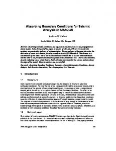
INTRODUCTION The Humboldt Bay Middle Channel Bridge (Fig. 1) is one of three bridges that cross Humboldt Bay on California State Route 255. Owned and maintained by the California Department of Transportation (Caltrans), the bridge (no 04-0229) is a 330 meter, nine-span composite structure with precast and prestressed concrete I-girders and cast-in-place concrete slabs to provide continuity. It is supported on eight pile groups, each of which consists of 5 to 16 prestressed concrete piles, in soils potentially vulnerable to liquefaction (under extreme earthquake shaking conditions). The river channel has an average slope from the banks to the center of about 7% (4 degrees). The foundation soil is composed mainly of dense fine-to-medium sand (SP/SM), organic silt (OL), and stiff clay layers (Fig. 2). In addition, thin layers of loose and soft clay (OL/SM) are located near the ground surface (see Fig. 2). The bridge was designed in 1968 and built in 1971 and has been the object of two Caltrans seismic retrofit efforts, the first one designed in 1985 and completed in 1987, and the second designed in 2001 to be completed in 2005. The objectives of the first retrofit effort were to mitigate the potential for unseating and diaphragm damage, while those of the second retrofit are to strengthen the piers, pilecaps, and pile groups. It is an interesting bridge because it is fairly representative of older AASHTO-Caltrans girder bridges with moderate traffic loads (average daily traffic of 4,600 to 15,800 in 1992), designed before ductile detailing was common. Furthermore, since the bridge is founded on poor soils, permanent ground deformation is a serious concern. Borehole 1 at Caltran’s Samoa Bridge Geotechnical downhole array (~0.25 mile north-west of the west abutment of the Middle Channel Bridge) provides a shear wave velocity profile down to a depth of 220 meters, where the borehole encountered bedrock (shear wave velocity > 850 m/sec). The shear wave velocities are about 180 m/sec in the upper 20 meters, lie in the range of 200 to 400 m/sec in the depth range of 20 to 60 meters, and fall in the range of 400 to 600 m/sec in the depth range of 60 to 220 meters (Somerville and Collins, 2002).
FIG. 1. Humboldt Bay Middle Channel Bridge (courtesy of Caltrans) FINITE ELEMENT MODELING A two-dimensional nonlinear model of the Middle Channel Bridge, including the superstructure, piers, and supporting piles was developed using OpenSees (McKenna and Fenves, 2001), as shown in Fig. 2 (Conte et al., 2002). The bridge piers are modeled using 2-D nonlinear material, fiber beam-column elements (with five Gauss-Lobato points along their length) formulated using the flexibility approach based on the exact interpolation of the internal forces (Spacone et al., 1996). The column cross-section is discretized into concrete and steel fibers. The uniaxial Kent-Scott-Park constitutive model with degraded linear unloading/reloading stiffness is used to model the concrete fibers, while the uniaxial bilinear model (or uniaxial J2 plasticity
2
model with linear kinematic hardening) is used to model the reinforcing steel. Confined and unconfined concrete materials are modeled using different sets of material constitutive parameters. The pile groups supporting the bridge piers are first lumped in the bridge transversal direction and then modeled using 2-D nonlinear material, fiber beam-column elements (with two Gauss-Lobato points in the length direction). The superstructure is idealized using equivalent linear elastic beam-column elements. The interior expansion joints and the abutment joints are modeled using zero-length elasto-plastic gap-hook elements. The soil domain is analyzed under the assumption of plane strain condition. It is spatially discretized using four-noded, bilinear, isoparametric finite elements with four integration points each. The materials in the various layers of the soil domain are modeled using a multi-surface plasticity model incorporating liquefaction effects and formulated in effective stresses (Elgamal et al., 2003). The lateral and base boundary conditions for the computational soil domain are modeled using a modified Lysmer transmitting/absorbing boundary. A set of viscous dampers normal and tangential to the soil boundaries is used to implement these transmitting boundaries.
Eureka Channel (South-East)
1
2
3
4
5
6
7
Samoa Channel (North-West)
8
A
B
FIG. 2. OpenSees finite element model of structure-foundation-soil system (based on blue prints courtesy of Caltrans, mesh generated using GID software) LYSMER-KUHLEMEYER TRANSMITTING/ABSORBING BOUNDARY For numerical accuracy, the maximum dimension of any soil element must be limited to one-eighth thru one-fifth of the shortest wavelength considered in the analysis. For computational efficiency, on the other hand, it is desirable to decrease the size of the soil domain included in the finite element model. As the size of the soil domain decreases, the treatment of its boundary conditions becomes increasingly more important. At the site of the Humboldt Bay Middle Channel Bridge, bedrock lies about 220 meters below the ground surface. In reality, the wave energy traveling away from the bridge site is dissipated by the soil medium and is never reflected back into the computational domain. In the finite element model developed, the soil domain is 1100 meters in length and 75 meters in depth. Since the soil domain is of finite size, the Lysmer-Kuhlemeyer boundary (Lysmer and Kuhlemeyer, 1969) is used to limit spurious wave reflections at the soil mesh boundary. This boundary absorbs the propagating waves in such a way that the incident wave is transmitted entirely into the soil domain of the finite element model without distortion and no waves are transmitted back to the exterior domain. The one-dimensional vertical shear wave equation can be written in the form 2 ∂ 2 u ( x, t ) 2 ∂ u ( x, t ) = vs ∂t 2 ∂x 2
(1)
where u denotes the soil particle displacement (perpendicular to the direction of wave propagation)
3
and v s = G ρ is the shear wave velocity. The solution of the above wave equation has the form
u ( x, t ) = u r (t −
x x ) + u i (t + ) vs vs
(2)
where ur(…) and ui(…) can be any arbitrary functions of (t − x v s ) and (t + x v s ) , respectively. The term u r (t − x v s ) represents the wave traveling at velocity vs in the positive x-direction, while u i (t + x v s ) represents the wave traveling at the same speed in the negative x-direction. Thus, ui is the incident wave if it points upwards into the computational domain and ur is the reflected wave. Taking the partial derivative with respect to time of both sides of the above equation and multiplying by ρv s gives
ρ vs
∂u ( x , t ) = ρvs ur' (t − x vs ) + ρvs ui' (t + x vs ) ∂t
(3)
where the prime superscript denotes the derivative of the associated function with respect to its argument. Now, the linear elastic uniaxial shear stress - shear strain relation is given by
τ ( x, t ) = G
∂u ( x, t ) G G = − u r' (t − x v s ) + u i' (t + x v s ) ∂x vs vs
(4)
where τ ( x, t ) is the shear stress. Combining equations (3) and (4), we get
τ ( x , t ) = − ρv s
∂u ( x, t ) + 2 ρv s u i' (t + x / v s ) ∂t
(5)
Note that ∂u ( x, t ) / ∂t represents the velocity of the total soil particle motion, while
u i' (t + x / v s ) = ∂u i (t + x / v s ) / ∂t is the velocity of the incident motion. Therefore, the first term on the right hand side of equation (5) is equivalent to the force (per unit area) generated by a dashpot of coefficient ρvs , while the second term is equivalent to a force (per unit area), which is proportional to the velocity of the incident wave. As a result, the soil below the soil domain of interest can be replaced with a dashpot and an equivalent force, which defines the seismic input. In our two-dimensional finite element model, we assume that the response of the soil deposit is predominantly caused by vertically propagating shear waves. We model the soil below the base (at a depth of about 75 m) of the computational domain as a linear elastic, undamped, and homogeneous semi-infinite half-space. It is expected that any nonlinearities below the base of the computational domain would remain small, since this soil is significantly stiffer than the soil within the computational domain. On each node at the base and on the lateral boundaries of the soil domain, we add two dashpots, normal and tangential to the boundary, respectively. The normal dashpots are set to absorb the reflected compressive waves while the tangential ones are set to absorb the reflected shear waves. And on each node at the base, an equivalent force, which is proportional to the velocity of the incident wave and the tributary surface area of the node, is applied in the horizontal direction to represent the vertically incident SV-wave.
4
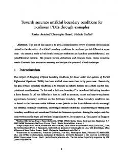
DEFINITION OF SEISMIC INPUT As we stated above, the seismic input is defined in terms of equivalent nodal forces (or effective earthquake forces), which are proportional to the velocity of the incident seismic wave, applied in the horizontal direction along the base of the soil domain included in the finite element model. Three sets of scaled actual earthquake ground motions corresponding to three different hazard levels (50%, 10%, and 2% in 50 years, respectively) including both soil and rock site conditions are used in the project (Somerville and Collins, 2002), yielding a total of 51 free surface ground motions. These free field ground motions are consistent with the local seismology at Humboldt Bay and with the magnitude-distance deaggregation of the seismic hazard, defined as the probability of the spectral acceleration at the fundamental period of the bridge-ground system exceeding a threshold level. For rock site free field ground motions, we assume that the free surface motion represents the rock outcropping motion. In the case of vertically propagating shear waves in a homogeneous, undamped, elastic half-space, the amplitude of the free surface total motion is twice the amplitude of the incident motion at any point in the half-space (Kramer, 1996). Thus, for each of the rock site ground motions, we take as incident seismic wave half the free surface ground motion. For the soil site free field ground motions, the software SHAKE (Schnabel et al, 1972) is used to deconvolve these free surface motions in order to obtain the corresponding incident wave motion at the base of the computational domain. For the deconvolution operation, it is assumed that the soil region underlying the soil domain included in the finite element model is homogeneous, viscoelastic, with material properties representative of the exterior soil domain. RESPONSE ANALYSIS To illustrate and validate the above procedure for defining the seismic input, a rectangular, homogeneous, undamped, elastic soil domain (1,100 by 40 meters in size) under plane stress condition is discretized into the finite element model shown in Fig. 3. Horizontal and vertical dashpots are defined at every node along the lateral and base boundaries of the soil domain. The dashpot coefficients (per unit area) are defined as ρvs and ρv p (where v p denotes the compressive or P-wave velocity) for the dashpots tangential and normal to the boundaries, respectively. Since we apply the results derived for one-dimensional wave propagation to a finite size two-dimensional soil domain, the soil domain is made sufficiently long so that the response in the center part of the mesh is close to its counterpart for the one-dimensional case. A sinusoidal incident wave is applied at the base through a set of nodal equivalent forces. The total acceleration response histories along the height of the two control soil columns shown in Fig. 3 are plotted in Fig. 4. We can clearly see the shear wave propagating vertically from the base to the top of the soil domain and being reflected at the free surface. The amplitude of the total acceleration on the ground surface is twice the amplitude of the incident wave. The vertical acceleration at points along the height of each control soil column remains very small compared to the horizontal acceleration at the same level, which verifies that the response of the soil domain is predominantly caused by vertically propagating shear waves. Thus, the results of one-dimensional wave propagation apply very well, even near the lateral boundaries (e.g., control soil column # 1), to the propagation of vertically incident shear waves through the finite size rectangular soil domain considered here and endowed with the Lysmer-Kuhlemeyer boundaries.
5
Soil Column #2
Soil Column #1
FIG. 3. Rectangular homogenous linear elastic soil domain It is more complicated to implement the Lysmer-Kuhlemeyer (L-K) transmitting/absorbing boundaries in the nonlinear soil domain of the bridge-ground system. In fact, since confining pressure dependent material plasticity models are used to model the behavior of the various soil layers, lateral confinement is needed for these soil layers to develop some strength. However, the dashpots cannot provide any lateral static constraint. Therefore, we need to proceed in several steps to apply the L-K boundaries for a static gravity analysis followed by a dynamic (earthquake response) analysis of the nonlinear bridge-ground system. First, we fix the base and lateral boundaries of the soil domain, set the various soil constitutive models to be linear elastic, and apply gravity. In the second step, the soil constitutive models are switched from linear elastic to elastoplastic accounting for liquefaction effects and the new static equilibrium state under gravity of the soil domain is obtained iteratively. Then the nonlinear material model of the bridge structure and foundations is added to the model of the soil domain and the gravity of the bridge is applied statically to the nonlinear bridge-ground system. In a third step, all the displacement constraints along the boundaries of the soil domain are removed and replaced with the corresponding support reactions recorded at the end of the second step. After balancing the internal and external forces, dashpots in both the horizontal and vertical directions are added to the base and lateral boundaries of the soil domain to model the L-K transmitting boundaries. Finally, in a fourth step, the seismic excitation is applied, in the form of equivalent nodal forces defined earlier, from the static equilibrium configuration under gravity loads. (a)
(b)
Horizontal acceleration Vertical acceleration
Ground surface motion
Horizontal acceleration Vertical acceleration
Total acceleration
Total acceleration
Ground surface motion
Incident wave 0
0.2
0.4
0.6
0.8
Time (sec)
1
1.2
1.4
Incident wave 1.6
0
0.2
0.4
0.6
0.8
Time (sec)
1
1.2
1.4
1.6
FIG. 4. Wave propagation through the rectangular homogeneous linear elastic soil domain, (a) control soil column # 1, (b) control soil column # 2 We investigated the wave propagation in the soil domain, shown in Fig. 5, of the bridge ground system, modeled as both a multi-layered linear elastic undamped and elastoplastic soil medium. A single Ricker wavelet with a dominant frequency of 3.9 Hz is used as the incident
6
wave, see Fig. 6. The total horizontal acceleration response histories at points along the height of the two control soil columns shown in Fig. 5 are plotted in Fig. 6. Observe that the amplitude of the linear response is greater than that of the nonlinear response and that the difference between these two response amplitudes decreases with depth. In both cases, the total acceleration response at the base of the soil domain is very close to that of the incident wave. For the linear case, we can clearly see the reflected incident wave reaching the base level, while for the nonlinear case the reflected wave dies out before it reaches the base. This is due to the fact that there is no source of energy dissipation in the linear soil, while energy is dissipated through inelastic action in the nonlinear soil. Soil Column #1
Soil Column #2
FIG. 5. Soil mesh of the Humboldt Bay Middle Channel Bridge (a)
(b)
Linear soil Nonlinear soil
Ground surface motion
Linear soil Nonlinear soil
Total horizontal acceleration
Total horizontal acceleration
Ground surface motion
Incident wave 0
0.5
1
Time (sec)
1.5
Incident wave 2
0
0.5
1
Time (sec)
1.5
2
FIG. 6. Linear soil versus nonlinear soil total horizontal acceleration response (single Ricker wavelet as incident wave, no bridge present), (a) control soil column # 1, (b) control soil column # 2 Before implementing the transmitting/absorbing L-K boundaries in our current (second generation) model of the Humboldt Bay bridge-foundation-soil system, in our first generation model of this bridge system, we implemented a shear beam constraint across the horizontal direction of the soil domain. According to this shear beam constraint, the two lateral boundaries (vertical sides) of the soil domain are constrained to deform similarly in the lateral direction by imposing equal horizontal degree of freedom constraints to pairs of lateral nodes at the same elevation. Then, the seismic input is applied to all nodes at the base of the soil domain assuming that the base moves rigidly according to the total ground acceleration input, thus neglecting spatial variability of the seismic input. It is of interest to compare the response simulation results obtained using the two types of soil boundary conditions and definition of the seismic input. Comparative results are shown in Figs. 7, 8, and 9. Fig. 7 corresponds to simulation cases without the bridge, while Figs. 8 and 9 show results of simulation cases with the bridge present. The total horizontal acceleration response histories at points along the height of control soil columns # 1
7
and 2 due to a single Ricker wavelet incident motion applied to the nonlinear soil without the bridge are shown in Fig. 7 for the two models of the soil boundary conditions and seismic input. Fig. 7 indicates that the soil acceleration responses for the two treatments of boundary conditions and seismic input are very close when the shear wave velocity of the soil below the computational soil domain is high (i.e., vs = 600 m/sec). Then, an actual earthquake ground motion record (with a 2% in 50 years hazard level), was applied as incident wave motion to the bridge-ground system. Fig. 8 compares the soil total horizontal acceleration response at points along the height of control soil columns # 1 and 2 for the two models of the soil boundary conditions and seismic input. The transmitting/absorbing L-K boundaries were based on a shear wave velocity of vs = 600 m/sec. A more significant difference between the soil responses for the two modeling assumptions is observed than in the case of the single wavelet incident motion (see Fig. 7). This could be due to the presence of the bridge structure and its foundations and/or to the fact that earthquake excitation has a greater frequency bandwidth than the Ricker wavelet considered and that high frequency waves are more sensitive to soil heterogeneities than relatively low frequency waves. Figs. 9 (a) and (b) show the shear stress – shear strain soil response during the earthquake at control points A and B, respectively, of the computational domain (see Fig. 2) for the two models of the soil boundary conditions and seismic input. Comparison of the responses of the bridge structure itself for both modeling assumptions is of the highest interest in this study. As an illustration, Fig. 9(c) shows the top-to-bottom relative horizontal displacement of the bridge column # 4 (see Fig. 2), while Fig. 9(d) displays the moment-curvature history of the base section of the bridge column # 1 (see Fig. 2). From Figs. 9, it is clear that the treatment of the soil boundary conditions and seismic input has a significant effect on the simulated local response of the soil material and response of the bridge structure itself. (a)
(b)
Shear Beam Transmitting/absorbing,Vs=600m/sec Transmitting/absorbing,Vs=300m/sec
Total horizontal Acceleration
Total horizontal Acceleration
Shear Beam Transmitting/absorbing,Vs=600m/sec Transmitting/absorbing,Vs=300m/sec
Incident wave 0
0.2
0.4
0.6
0.8
Time (sec)
1
Incident wave 1.2
1.4
0
0.2
0.4
0.6
0.8
Time (sec)
1
1.2
1.4
FIG. 7. Nonlinear soil total horizontal acceleration response at points along the two control soil columns (single Ricker wavelet as incident wave, no bridge present), (a) control soil column #1, (b) control soil column # 2
8
Shear Beam Transmitting/absorbing
(b)
Shear Beam Transmitting/absorbing
Total horizontal acceleration
Total horizontal acceleration
(a)
Incident wave 0
Incident wave
5
10
15
Time (sec)
(c)
20
0
Shear Beam Transmitting/absorbing
5
10
(d)
20
Shear Beam Transmitting/absorbing
Total horizontal acceleration
Total horizontal acceleration
15
Time (sec)
Incident wave 8
8.5
9
9.5
10
Incident wave 10.5
Time (sec)
11
11.5
12
8
8.5
9
9.5
10
10.5
Time (sec)
11
11.5
12
FIG. 8. Nonlinear soil total horizontal acceleration response at points along the two control soil columns (earthquake ground motion as incident wave, bridge present), (a) control soil column # 1, (b) control soil column # 2 , (c) zoom of (a), (d) zoom of (b) 80
10
(a)
60 40 Shear stress (KPa)
Shear stress (KPa)
5
0
20 0 −20 −40
−5
−60
Shear Beam Boundary Transmitting/Absorbing Boundary −10
(b)
−0.002
0 0.002 Shear strain
−80 −0.004
0.004
9
Shear Beam Boundary Transmitting/Absorbing Boundary −0.002
0 0.002 Shear strain
0.004
0.006
Base section of column #1
Column #4 10000
0.2 Shear Beam Boundary Transmitting/Absorbing Boundary
(c)
8000
(d)
0.15
Moment (KN−M)
Moment (KN−M)
6000
0.1
0.05
0
4000 2000 0 −2000 −4000
−0.05
−0.1 0
−6000
10
20
30
40
50
60
−8000 −0.004
70
Shear Beam Boundary Transmitting/Absorbing Boundary −0.002
0
0.002
0.004
0.006
0.008
Curvature
Time (sec)
FIG. 9. Nonlinear soil and bridge structure responses (earthquake motion as incident wave), (a) shear stress –shear strain soil response at control point A (see Fig. 2), (b) shear stress – shear strain soil response at control point B (see Fig. 2), (c) top-bottom horizontal relative displacement of bridge column # 4, (d) moment-curvature at base section of bridge column #1 CONCLUSIONS This paper briefly describes a 2D nonlinear finite element model of the structure-foundation-soil system for the Middle Channel Bridge at Humboldt Bay near Eureka in Northern California. This model was developed using OpenSees, the new software framework for seismic response simulation of structural and geotechnical systems developed by the Pacific Earthquake Engineering Research (PEER) Center. This paper especially focuses on the implementation of the Lysmer-Kuhlemeyer transmitting/absorbing boundary for this bridge model. Several response simulations were conducted to verify this implementation. The effect of linear elastic versus elastoplastic soil constitutive behavior on the propagation of vertically incident shear waves in the computational domain is examined. It is found that soil nonlinearity has a significant effect on the wave propagation through the foundation soil. The difference between two approximate modeling approaches for the soil boundary conditions and definition of the seismic input was investigated in terms of local and global, soil and bridge structure responses to vertically incident shear waves. These two modeling approaches are: (1) shear beam constraints across the longitudinal direction of the computational soil domain used in conjunction with “rigid soil” excitation under the base of the computational soil domain; and (2) use of Lysmer-Kuhlemeyer transmitting/ absorbing boundaries along the lateral sides and base of the computational soil domain in conjunction with a definition of the seismic input in terms of vertically incident shear waves. It is found that these two modeling approaches can produce quite different responses of the bridge structure itself. This study is part of the PEER Center ongoing development of a probabilistic seismic performance assessment methodology for civil structures such as buildings and highway bridges. This methodology integrates probabilistic seismic hazard analysis, advanced computational modeling of the bridge ground system, probabilistic seismic demand analysis, and probabilistic damage analysis or fragility analysis (Cornell and Krawinkler, 2000).
10
ACKNOWLEDGMENTS Support of this work was provided primarily by the Earthquake Engineering Research Centers Program of the National Science Foundation, under Award Number EEC-9701568 through the Pacific Earthquake Engineering Research Center (PEER). This support is gratefully acknowledged. The authors wish to thank Mr. Patrick Hipley, Mr. Cliff Roblee, Mr. Charles Sikorsky, and Mr. Mark Yashinsky of Caltrans for providing all the requested information regarding the initial design and retrofits of the Middle Channel Bridge. Prof. Greg Fenves, Dr. Frank McKenna, Mr. Michael Scott (U.C. Berkeley) and Prof. Boris Jeremic (U.C. Davis) helped with the OpenSees modeling and analysis framework. Prof. Pedro Arduino (Univ. of Washington, Seattle) suggested and helped with the use of GID (http://gid.cimne.upc.es/), a commercial preand post-processing system for geometric modeling and visualization. Their help is gratefully acknowledged. REFERENCES Conte, J.P., A. Elgamal, Z. Yang, Y. Zhang, G. Acero, and F. Seible (2002), "Nonlinear Seismic th Analysis of a Bridge Ground System," (CD-ROM), Proceedings of the15 ASCE Engineering Mechanics Conference, Columbia University, New York, June 2-5, 2002. Cornell, C.A. and H. Krawinkler (2000), "Progress and Challenges in Seismic Performance Assessment," PEER Center News, 3(2), Spring 2000. Elgamal, A., Z. Yang, E. Parra, and A. Ragheb (2003), "Modeling of Cyclic Mobility in Saturated Cohesionless Soils," International Journal of Plasticity, 19(6), 883-905. Kramer, S. L. (1996), Geotechnical Earthquake Engineering, Prentice Hall, Upper Saddle River, New Jersey, USA. Lysmer, J., and R.L. Kuhlemeyer (1969), “Finite Dynamic Model for Infinite Media,” Journal of the Engineering Mechanics Division, ASCE, 95(EM4), 859-877. McKenna, F. and G.L. Fenves (2001), "The OpenSees Command Language Manual, Version 1.2," Pacific Earthquake Engineering Research Center, University of California at Berkeley, Berkeley, CA (http://opensees.berkeley.edu/ ). Schnabel, P.B., J. Lysmer, and H.B. Seed (1972), “SHAKE: A Computer Program for Earthquake Response Analysis of Horizontally Layered Sites”, Report No. EERC 72-12, Earthquake Engineering Research Center, University of California, Berkeley, CA. Somerville, P., and N. Collins (2002), “Ground Motion Time Histories for the Humboldt Bay Bridge,” Report of the PEER Performance Based Earthquake Engineering Methodology Testbed Program, Pacific Earthquake Engineering Research Center, University of California at Berkeley, Berkeley, CA (http://peer.berkeley.edu/ ). Spacone, E., F.C. Filippou, and F.F. Taucer (1996), " Fibre Beam-Column Model for Non-Linear Analysis of R/C Frames: Part I. Formulation," Earthquake Engineering and Structural Dynamics, 25 (7), 711-725.
11