Trimming, Mapping, and Optimization in Isogeometric

T ECHNISCHE U NIVERSITÄT M ÜNCHEN Lehrstuhl für Statik

Trimming, Mapping, and Optimization in Isogeometric Analysis of Shell Structures Robert Schmidt

Vollständiger Abdruck der von der Ingenieurfakultät Bau Geo Umwelt der Technischen Universität München zur Erlangung des akademischen Grades eines Doktor-Ingenieurs genehmigten Dissertation.

Vorsitzender:

Univ.-Prof. Dr.-Ing. habil. Fabian Duddeck

Prüfer der Dissertation: 1. Univ.-Prof. Dr.-Ing. Kai-Uwe Bletzinger 2. Univ.-Prof. Dr. rer. nat. Ernst Rank 3. Prof. Alessandro Reali, Ph.D., Università degli Studi di Pavia, Italien

Die Dissertation wurde am 23.04.2013 bei der Technischen Universität München eingereicht und durch die Ingenieurfakultät Bau Geo Umwelt am 23.07.2013 angenommen.

III

Abstract The design and the analysis of thin-walled structures rely on the quality of the geometric models. Isogeometric Analysis provides a natural framework in considering both models as one. Consequently, geometrical errors are excluded by construction. In order to extend the applicability of Isogeometric Analysis, a combination of reconstruction and coupling methods is proposed to perform analysis on trimmed NURBS surfaces. This approach comprises trimmed single and multi-patch surfaces. The performance of this new methodology is highlighted in various examples. Moreover, a new concept, denoted as Isogeometric Load Design, is derived. This method enables to define areas of arbitrary shape to be subjected to a given loading. In particular, these loading areas do not have to conform with the underlying parameterization. Thus, a new feature is added to the framework of integrated design and analysis. Another aspect in the design and analysis of thin-walled structures deals with shape optimization. It can be shown that Isogeometric Analysis and Shape Optimization merge naturally. Moreover, the equality of the involved models provides several advantages compared to the classical approaches. Additionally, it is demonstrated that only the coefficients of a gradient field and not the discrete gradient vectors should be applied to update the design. Otherwise, the influence of the individual design variables and its basis functions is not correctly reflected. In a next step, Isogeometric Shape Optimization is extended from single patch problems to multi-patches. The need for a continuity constraint on the optimization model is delineated and a variational formulation of this constraint is introduced. This formulation provides the possibility to handle design models consisting of conforming and nonconforming multi-patches. At several examples, it is highlighted that this constraint can be used to perpetuate continuity across patch boundaries. Moreover, it is shown that initial non-smoothly joined patches can be transformed during the optimization procedure into a smooth multi-patch shape.

IV

Zusammenfassung Das Design als auch die Analyse von dünnen Strukturen basieren auf geometrischen Modellen und hängen somit von deren Eigenschaften ab. Die Isogeometrische Analyse stellt das Geometrie- und Analysemodell auf eine einheitliche Basis, wodurch von Beginn an geometrische Fehler ausgeschlossen werden können. Um den Einsatzbereich der Isogeometrischen Analyse auf getrimmte NURBS Flächen zu erweitern, wird eine Kombination aus Rekonstruktions- und Kopplungsmethoden vorgeschlagen. Besonderen Wert wird darauf gelegt, dass nicht nur einzelne getrimmte NURBS Flächen, sondern auch Flächen, die aus mehreren getrimmten NURBS bestehen, verwendet werden können. Die besondere Eignung dieses neuen Ansatzes wird an verschiedenen Beispielen herausgestellt. Darüber hinaus wird ein neues Konzept, namens Isogeometric Load Design, zur Aufbringung von Lasten präsentiert. Dieser neue Ansatz ermöglicht es, Lasten jeglicher Form unabhängig von der eigentlichen Parametrisierung einer NURBS Fläche zu definieren und kann dadurch als weiterer Baustein im integrierten Design- und Analyseprozess gesehen werden. Die Formoptimierung ist ein wichtiges Instrument bei der Formgebung und der Analyse von dünnen Schalenstrukturen. Durch die Anwendung der Isogeometrischen Analyse in der Formoptimierung können Geometrie-, Optimierungs-, und Analysemodell vereinheitlicht werden, wodurch sich Vorteile gegenüber den klassischen Ansätzen ergeben. Im Rahmen dieser Arbeit wird gezeigt, dass bei der Sensitivitätsanalyse der Zielfunktion der Einflussbereich der einzelnen Designvariablen mit in Betracht gezogen werden muss. Um dies zu gewährleisten, wird die Sensitivität einer Designvariablen mit dem Integral der zugehörigen Ansatzfunktion gewichtet. Wie schon bei der Analyse getrimmter NURBS Patches wird darauf geachtet, dass die Methodik nicht auf einzelne NURBS Patches beschränkt bleibt. Um die isogeometrische Formoptimierung auf mehrere NURBS Patches erweitern zu können, muss das Optimierungsmodell mit Kontinuitätsbedingungen am Übergang von einem NURBS Patch zum anderen versehen werden. Zur Umsetzung dieser Zwangsbedingung wird eine variationelle Formulierung angewandt. Dieser Ansatz bietet die Möglichkeit, die Kontinuität des Optimierungsmodells von konformen als auch von nichtkonformen NURBS Patches zu erhalten. Des Weiteren können mit diesem Ansatz vorhandene Knicke am Übergang der NURBS Patches während des Optimierungsvorgangs eliminiert werden.

V

Acknowledgments This thesis was written during my time as a research scholar at the Chair of Structural Analysis at the Technische Universität München. First of all, I would like to express my deep gratitude to Professor Dr.-Ing. Kai-Uwe Bletzinger, my research supervisor, for the opportunity to join his research group and the possibility to work in the fascinating and fast growing research area of Isogeometric Analysis. I also appreciate the useful critiques of this research work. Furthermore, I would like to address my thanks to the members of my examining jury, Univ.-Prof. Dr. rer. nat. Ernst Rank and Prof. Alessandro Reali. Their interest in my work is gratefully appreciated. Also, I want to thank Prof. Dr.-Ing. habil. Fabian Duddeck for chairing the jury. I would also like to thank Dr.-Ing. Roland Wüchner, for his advice, assistance, and support during my PhD as well as during my studies at TUM. I would like to extend my thanks to my colleagues - especially to my roommates - for having a good time at the chair throughout my PhD period. In particular, I want to address many thanks to Dr.-Ing. Josef Kiendl for introducing me into Isogeometric Analysis as well as for the collaboration and support. The funding for my whole work as research scholar was granted by the International Graduate School of Science and Engineering (IGSSE) and is gratefully acknowledged. Last but not least, I wish to thank my parents for all their love and support at all times.

Munich, August 2013

Robert Schmidt

Table of Contents

Abstract

III

Zusammenfassung

IV

1 Introduction 1.1 Motivation . . . . . . . . . . . . . . . . . . . . . . . . . . . . . . . . . . . . . 1.2 Contributions . . . . . . . . . . . . . . . . . . . . . . . . . . . . . . . . . . . 1.3 Outline . . . . . . . . . . . . . . . . . . . . . . . . . . . . . . . . . . . . . . . 2 Theoretical basics of NURBS 2.1 Historical Background . . 2.2 B-Splines . . . . . . . . . . 2.2.1 Parametric domain 2.2.2 Basis function . . . 2.2.3 Geometry entities . 2.3 NURBS . . . . . . . . . . . 2.3.1 Definition . . . . . 2.3.2 Continuity . . . . . 2.4 Trimmed NURBS . . . . .

. . . . . . . . .

. . . . . . . . .

. . . . . . . . .

. . . . . . . . .

3 Basics of mechanics 3.1 Structural Mechanics . . . . . . . 3.1.1 Kinematics . . . . . . . . . 3.1.2 Constitutive equation . . 3.1.3 Boundary Value Problem 3.2 The Finite Element Method . . . 3.2.1 Weak Form . . . . . . . . 3.2.2 Discretization . . . . . . .

. . . . . . . . . . . . . . . .

4 Isogeometric Analysis 4.1 Attributes . . . . . . . . . . . . . . 4.2 Element definition and Integration 4.3 Refinement . . . . . . . . . . . . . . 4.4 Element formulation . . . . . . . . 4.4.1 Assumptions . . . . . . . . 4.4.2 Kinematics . . . . . . . . . . 4.4.3 FE-equations . . . . . . . .

. . . . . . . . . . . . . . . . . . . . . . .

. . . . . . . . . . . . . . . . . . . . . . .

. . . . . . . . . . . . . . . . . . . . . . .

. . . . . . . . . . . . . . . . . . . . . . .

. . . . . . . . . . . . . . . . . . . . . . .

. . . . . . . . . . . . . . . . . . . . . . .

. . . . . . . . . . . . . . . . . . . . . . .

. . . . . . . . . . . . . . . . . . . . . . .

. . . . . . . . . . . . . . . . . . . . . . .

. . . . . . . . . . . . . . . . . . . . . . .

. . . . . . . . . . . . . . . . . . . . . . .

. . . . . . . . . . . . . . . . . . . . . . .

. . . . . . . . . . . . . . . . . . . . . . .

. . . . . . . . . . . . . . . . . . . . . . .

. . . . . . . . . . . . . . . . . . . . . . .

. . . . . . . . . . . . . . . . . . . . . . .

. . . . . . . . . . . . . . . . . . . . . . .

. . . . . . . . . . . . . . . . . . . . . . .

. . . . . . . . . . . . . . . . . . . . . . .

. . . . . . . . . . . . . . . . . . . . . . .

. . . . . . . . . . . . . . . . . . . . . . .

. . . . . . . . . . . . . . . . . . . . . . .

1 1 3 3

. . . . . . . . .

5 5 7 7 7 8 9 9 11 12

. . . . . . .

17 17 17 19 19 20 20 21

. . . . . . .

25 25 28 28 30 30 30 32

VIII

5 Coupling of nonconforming discretizations 5.1 Coupling methods . . . . . . . . . . . . 5.1.1 Interpolation Method . . . . . . 5.1.2 Discrete Least-Squares Method . 5.1.3 Weighted-Residual Method . . . 5.2 Field approximation . . . . . . . . . . . 5.3 Mapping quantities . . . . . . . . . . . . 5.3.1 State mapping . . . . . . . . . . . 5.3.2 Force mapping . . . . . . . . . . 5.4 Numerical investigations . . . . . . . . . 5.4.1 State mapping . . . . . . . . . . . 5.4.2 Force mapping . . . . . . . . . . 5.5 Concluding remarks . . . . . . . . . . .

Table of Contents

. . . . . . . . . . . .

. . . . . . . . . . . .

. . . . . . . . . . . .

. . . . . . . . . . . .

. . . . . . . . . . . .

6 Isogeometric Analysis of trimmed NURBS surfaces 6.1 Basic ideas of the method . . . . . . . . . . . . . 6.2 Algorithmic formulation . . . . . . . . . . . . . . 6.3 Assessment of the reconstruction . . . . . . . . . 6.4 Finite element equations . . . . . . . . . . . . . . 6.5 Boundary conditions . . . . . . . . . . . . . . . . 6.5.1 Neumann . . . . . . . . . . . . . . . . . . 6.5.2 Dirichlet . . . . . . . . . . . . . . . . . . . 6.6 Conditioning of the system matrix . . . . . . . . 6.6.1 Problem description . . . . . . . . . . . . 6.6.2 Preconditioning . . . . . . . . . . . . . . . 6.6.3 Plate example . . . . . . . . . . . . . . . . 6.6.4 Concluding remarks . . . . . . . . . . . . 6.7 Benchmarking . . . . . . . . . . . . . . . . . . . . 6.7.1 Cantilever plate . . . . . . . . . . . . . . . 6.7.2 Cantilever plate with curved edge . . . . 6.7.3 Trimmed cylinder shell . . . . . . . . . . 6.7.4 Doubly-curved surface . . . . . . . . . . . 7 Isogeometric Analysis of trimmed multi-patches 7.1 C0 -continuity . . . . . . . . . . . . . . . . . . 7.2 G1 -continuity . . . . . . . . . . . . . . . . . . 7.3 Benchmarking . . . . . . . . . . . . . . . . . . 7.3.1 Tension test . . . . . . . . . . . . . . . 7.3.2 Cantilever plate . . . . . . . . . . . . . 7.3.3 Trimmed quarter-cylinders . . . . . . 7.3.4 Trimmed Hemisphere . . . . . . . . .

. . . . . . .

. . . . . . .

. . . . . . . . . . . .

. . . . . . . . . . . . . . . . .

. . . . . . .

. . . . . . . . . . . .

. . . . . . . . . . . . . . . . .

. . . . . . .

. . . . . . . . . . . .

. . . . . . . . . . . . . . . . .

. . . . . . .

. . . . . . . . . . . .

. . . . . . . . . . . . . . . . .

. . . . . . .

8 Isogeometric Analysis and triangular Bézier shell elements 8.1 Triangular Bézier functions . . . . . . . . . . . . . . . . 8.2 Element formulation . . . . . . . . . . . . . . . . . . . . 8.3 Integration . . . . . . . . . . . . . . . . . . . . . . . . . . 8.4 Continuity enforcement . . . . . . . . . . . . . . . . . . 8.5 Benchmarking . . . . . . . . . . . . . . . . . . . . . . . . 8.5.1 Scordelis-Lo roof . . . . . . . . . . . . . . . . . . 8.5.2 Pinched Cylinder . . . . . . . . . . . . . . . . . .

. . . . . . . . . . . .

. . . . . . . . . . . . . . . . .

. . . . . . .

. . . . . . .

. . . . . . . . . . . .

. . . . . . . . . . . . . . . . .

. . . . . . .

. . . . . . .

. . . . . . . . . . . .

. . . . . . . . . . . . . . . . .

. . . . . . .

. . . . . . .

. . . . . . . . . . . .

. . . . . . . . . . . . . . . . .

. . . . . . .

. . . . . . .

. . . . . . . . . . . .

. . . . . . . . . . . . . . . . .

. . . . . . .

. . . . . . .

. . . . . . . . . . . .

. . . . . . . . . . . . . . . . .

. . . . . . .

. . . . . . .

. . . . . . . . . . . .

. . . . . . . . . . . . . . . . .

. . . . . . .

. . . . . . .

. . . . . . . . . . . .

. . . . . . . . . . . . . . . . .

. . . . . . .

. . . . . . .

. . . . . . . . . . . .

. . . . . . . . . . . . . . . . .

. . . . . . .

. . . . . . .

. . . . . . . . . . . .

. . . . . . . . . . . . . . . . .

. . . . . . .

. . . . . . .

. . . . . . . . . . . .

33 33 33 34 35 36 37 37 37 38 40 42 51

. . . . . . . . . . . . . . . . .

53 53 54 61 62 66 66 67 68 68 69 70 71 71 71 72 75 75

. . . . . . .

81 81 84 86 86 88 90 90

. . . . . . .

95 96 98 99 99 100 100 102

Table of Contents

8.6

8.7

8.5.3 Pinched Hemisphere . . . . . . . . . . . . . 8.5.4 Bending a cantilever plate to a cylinder . . 8.5.5 Pullout of an open-ended cylindrical shell Analysis of trimmed NURBS surfaces . . . . . . . 8.6.1 Infinite plate with hole . . . . . . . . . . . . 8.6.2 Wide-spanning roof-like structure . . . . . Concluding remarks . . . . . . . . . . . . . . . . .

IX

. . . . . . .

. . . . . . .

. . . . . . .

. . . . . . .

. . . . . . .

. . . . . . .

. . . . . . .

. . . . . . .

. . . . . . .

. . . . . . .

. . . . . . .

. . . . . . .

. . . . . . .

. . . . . . .

103 105 105 106 108 111 111

9 Isogeometric Shape Optimization 9.1 Optimization problem . . . . . . . . . . . . . . . . . . . . 9.2 Isogeometric Optimization concept . . . . . . . . . . . . . 9.3 Sensitivity Analysis . . . . . . . . . . . . . . . . . . . . . . 9.3.1 Discrete semi-analytical Sensitivities . . . . . . . . 9.3.2 Gradient of the objective function . . . . . . . . . 9.3.3 Study on sensitivity weighting . . . . . . . . . . . 9.4 Study on the directional dependency of optimal solutions 9.4.1 Square plate . . . . . . . . . . . . . . . . . . . . . . 9.4.2 Circular disk . . . . . . . . . . . . . . . . . . . . . .

. . . . . . . . .

. . . . . . . . .

. . . . . . . . .

. . . . . . . . .

. . . . . . . . .

. . . . . . . . .

. . . . . . . . .

. . . . . . . . .

. . . . . . . . .

. . . . . . . . .

113 114 115 116 116 118 120 122 122 123

10 Isogeometric Shape Optimization with multi-patches 10.1 Problem statement . . . . . . . . . . . . . . . . . . . . 10.2 Constraint formulation . . . . . . . . . . . . . . . . . . 10.2.1 Continuity constraint . . . . . . . . . . . . . . . 10.3 Perpetuation of Geometric Continuity . . . . . . . . . 10.4 Enforcement of Geometric Continuity . . . . . . . . . 10.5 Comparison between single patch and multi-patches 10.6 Nonconforming Optimization models . . . . . . . . . 10.6.1 Choice of integration domain . . . . . . . . . . 10.6.2 Perpetuation of Tangent Continuity . . . . . . 10.6.3 Enforcement of Tangent Continuity . . . . . .

. . . . . . . . . .

. . . . . . . . . .

. . . . . . . . . .

. . . . . . . . . .

. . . . . . . . . .

. . . . . . . . . .

. . . . . . . . . .

. . . . . . . . . .

. . . . . . . . . .

. . . . . . . . . .

129 129 130 132 133 134 137 140 143 144 146

. . . . . . . . . .

. . . . . . . . . .

11 Conclusion

153

Appendix A Geometric data of models

157

Appendix B Integration points for polynomials on triangular domains

159

Bibliography

165

Chapter

1

Introduction 1.1 Motivation The design of structures like aircraft or motor vehicles is one of the big challenges nowadays. Those have to be bigger, more efficient, and more powerful than the already existing ones. Moreover, they have to conform with economic and environmental needs. The path from the first drafts to the final realization demands a strong interaction between the involved engineers. The reason is that the product has to obey all the demands derived from aesthetic, functional, reliability, manufacturing, and sustainability considerations. This thesis focuses on the interaction between the design, as derived out of functional aspects, and the analysis of a structure. Nowadays, the field of lightweight design becomes more and more important. Lightweight design approaches produce structures, which are not only lighter but also exploiting optimally the given material properties. A prominent example of such structural elements is a shell. A shell is characterized by the fact that its thickness is small compared to its other dimensions. Additionally, its stiffness is mainly defined by its geometry rather than by its material. Thus, the combination of an optimally shaped shell and a material with a high strength resistance, e.g., carbon fiber reinforced plastics (CFRP), are perfectly suited for lightweight designs. These properties attribute to save material, which has obvious advantages concerning economic and environmental aspects. Applying lightweight design concepts, an advanced knowledge in mechanics is demanded from the designer. In particular, recognizing areas of high stress concentration and actions to remedy those should to be known by a designer. The advent of computers in engineering problems made it possible to generate different designs and perform detailed studies on them. Moreover, mathematical optimization techniques are supporting the search of optimal shapes for structures subjected to some mechanical constraints, e.g., stresses. Although it is known that the design and the analysis of structures strongly depend on each other, there is no common basis in which they are described. This has historical reasons. The predominant technology in structural mechanics is the Finite Element Method, see, for example, Bathe [2002], Hughes [2000], or Zienkiewicz et al. [2005]. The first publications can be dated back to the mid 1950s. Since its early days, the most common approach is to decompose the continuous analysis model into a finite set of elements, which comprise linear polynomials. On the contrary, the geometric basis for the design are mostly parametric splines. A spline in one dimension is a set of curves with an arbitrary basis, e.g., polynomial, which are joined smoothly at their ends. The re-

2

Introduction

quirement to attain the computer model of a geometry has its roots in the 1950s. At that time, numerically-controlled production machines were introduced and demanded for a smooth description of the parts to be manufactured. The first software which allowed to create a geometric model within a computer system can be traced back to the PhD thesis of Sutherland [1963]. Another advantage of geometric models represented with splines was that blue prints were no longer needed. Instead, the geometry could be stored numerically, which made it easier and more precise to be reproduced. The delayed development of CAGD methods compared to the FEM resulted in a different geometric formulation of the computational models. Consequently, structures, generated in a Computer-Aided Design (CAD) environment, have to be converted into a model suited for the analysis. Although highly automated mesh generators exist today, several iterations and adjustments are required to obtain a finite element mesh with the desired quality. Before the advent of Isogeometric Analysis, splines had been already used to solve variational problems, see, for example, Höllig et al. [2001], Höllig and Reif [2003], or Höllig [2003]. In the beginning of the 2000s, a popular technology in Computer Graphics, i.e., Subdivision Surfaces, has been used for the analysis and it was realized that Subdivision Surfaces are integrating modeling and analysis. See Cirak et al. [2000, 2002] for the corresponding references. In the research community, the breakthrough of the splinebased Finite Element methodology came with the publication of Hughes et al. [2005]. They employed Non-Uniform Rational B-Splines (NURBS) as a basis for the Finite Element Analysis and coined this type of method "Isogeometric Analysis". Since NURBS are de facto the standard in geometric modeling, this methodology naturally combines Computer-Aided Design and Computer-Aided Engineering. Although young of age, a tremendous amount of publications has been published regarding Isogeometric Analysis since then. A nice overview about its capabilities is provided in the first textbook about Isogeometric Analysis in Cottrell et al. [2009]. Using the parameterization of the geometric model directly for the analysis poses the question of suitability of the analysis model. The effect of different parameterization on the solution has been investigated in Cohen et al. [2010], and Schmidt et al. [2010]. Another drawback is that the geometric models do not always provide all the information needed for an analysis. For instance, in a CAD environment no parameterization of volumes is being used. Instead, a Boundary representation (B-rep) technique is applied, i.e., only the bounding surfaces are generated and represented. Thus, the missing parameterization has to be created. For example, in Aigner et al. [2009], and Zhang et al. [2012], two approaches to construct volume parameterizations for Isogeometric Analysis are presented. Trimmed NURBS patches also belong to this category. The associated patches are actually not trimmed but rather supplemented with trimming curves or surfaces. These additional curves and surfaces are only used for rendering the geometric model. Consequently, there is no definition of the computational domain. In the context of Isogeometric Analysis, Kim et al. [2009, 2010] proposed to define the integration domain of trimmed knots spans by using triangles. The integration technique for the triangles is borrowed from the NURBS-enhanced Finite Element Method, see, for example, Sevilla et al. [2008]. A different method is to use embedded domain methods, e.g., the Finite Cell Method. This method can be equipped with standard p-FEM and NURBS functions. Regarding Isogeometric Analysis, some selected contributions can be found in Rank et al. [2011, 2012] and Schillinger et al. [2012]. However, the initial objective of Isogeometric Analysis to provide a unified framework for the integration of CAD and

1.2 Contributions

3

CAE is not yet realized. The problem is that geometric models generally consist out of multiple trimmed patches for which suitable methods are still missing.

1.2 Contributions Within this thesis, coupling methods are employed in the context of Isogeometric Analysis of thin-walled structures. A new methodology based on the combination of a reconstruction technique and coupling methods is proposed to perform Isogeometric Analysis of trimmed NURBS surfaces. This method is not restricted to single patches. It is demonstrated that using the Bending Strip method in conjunction with the reconstruction approach also trimmed multi-patches can be analyzed. In addition, a different interpretation of this scheme allows to apply Neumann boundary conditions independently of the underlying parameterization in an intuitive and simple way. In particular, it is possible to "design" the load in the pre-processor. Consequently, this new approach is denoted as Isogeometric Load Design. In order to simplify the reconstruction and to avoid singular parameterization, a triangular element based on Bézier functions is introduced. It is shown that triangular Bézier elements provide accurate results independent of whether they are used for every knot span of a patch or only for the trimmed knot spans. Another area of application of coupling methods is the field of Isogeometric Shape Optimization of multiple patches. A variational continuity constraint formulation is proposed to handle matching and non-matching patches at the common interface. In addition to this contribution, the problem of applying the gradients directly as design update is delineated. To remedy this issue, it is proposed to weight each response sensitivity with the influence of the corresponding design variable. Moreover, it is pointed out that the optimization results using Isogeometric Analysis do not show any intrinsic mesh dependency.

1.3 Outline Chapter two provides a description of what B-Splines and NURBS are and how they are formulated. Additionally, some historical remarks are given. Moreover, the problem of trimmed NURBS patches is introduced and possible pitfalls in the analysis of trimmed NURBS surfaces are highlighted. In Chapter three, the basic formulation of the structural mechanics problem is delineated. Additionally, the Finite Element Method and its application to the mechanical problem are introduced. Chapter four contains an introduction to Isogeometric Analysis. Furthermore, a comparison to the standard Finite Element Method is performed. Moreover, the definition of finite elements in the context of Isogeometric Analysis is provided. In addition, the used Kirchhoff-Love shell element formulation is concisely presented. The basic concepts of coupling nonconforming NURBS discretizations are introduced within Chapter five. Moreover, a study on the quality of the investigated coupling schemes when mapping field and flux type quantities is performed for different combinations of

4

Introduction

polynomial degrees. The basic ideas of the approach to perform Isogeometric Analysis on trimmed NURBS surfaces are provided within Chapter six. Additionally, the corresponding formulation is presented. The theoretical development is supported by numerical examples, which highlight the accuracy and power of the proposed concept. Moreover, this chapter covers Isogeometric Load Design, a new approach to define loads on a NURBS patch independently of the underlying parameterization. Chapter seven extends the Isogeometric Analysis of trimmed NURBS surfaces to multipatch problems. Based on the reconstruction approach, the required steps to enforce point and tangent continuity are delineated. Numerical investigations confirm the applicability of the proposed approach. Chapter eight introduces triangular Bézier patches in the context of Isogeometric Analysis. It provides the basic description of the Bézier functions and the needed modifications of the NURBS-based Kirchhoff-Love shell element. It is demonstrated that the reconstruction approach easily maintains the continuity between the individual elements. The main purpose of this specific element type is to avoid singular points within a finite element and to ease the reconstruction procedure within the Isogeometric Analysis of trimmed NURBS surfaces. The concept of Isogeometric Shape Optimization is described in Chapter nine. This chapter investigates also the need to weight the sensitivities of the objective function in order to reflect the influence of each design variable. Moreover, a study on the directional dependency of optimal results on the underlying parameterization is performed. Chapter ten describes the problem of extending Isogeometric Shape Optimization to multipatch surfaces. The need of continuity constraints on the design models is described. The proposed formulation, i.e., a variational constraint, offers the possibility to employ also nonconforming patches in the design model. These possibilities are supported by numerical investigations. In Chapter eleven concluding remarks on the developments contained within this thesis are given. Moreover, an outlook for further research topics is provided.

Chapter

2

Theoretical basics of NURBS This chapter introduces the essential theoretical framework regarding the mathematical description of geometric models using Non-Uniform Rational B-Splines (NURBS). After some remarks to the historical development of splines, the basic definition of the B-Splines and their transformation to the NURBS are introduced. Furthermore, an introduction into the field of trimmed NURBS surfaces is provided. This thesis deals only with B-Splines and NURBS. In the CAGD, there are many other types of splines known, e.g., β-Splines and L-Splines. The interested reader is referred to the books of Farin et al. [2002] and Schumaker [2007] and the reference therein for details and other types of splines.

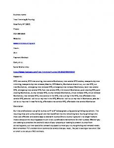
2.1 Historical Background When creating a new product, for instance, a bottle, house, car or boat, the fundamental question is: “How can the design be described?” In general, the design itself consists of many shapes, but mostly of geometric primitives like lines and ellipses. However, there exist other types of geometry which cannot be described by these primitives, the so-called free-form surfaces. They can be described by “splines”. In the early time, a spline was a thin, elastic wooden beam, see Figure 2.1, and was referred to as a mechanical spline. The shape of the spline is defined by interpolating specified points which are fixed by placing metal weights, the so-called "ducks", at the corresponding positions. This method is still

Figure 2.1: mechanical spline defined through placing ducks at defined positions. (Pictures are taken from www.boatdesign.de)

6

Theoretical basics of NURBS

Figure 2.2: de Casteljau alorithm. (Picture taken from Farin et al. [2002])

used to design small boats, as it can be seen in Figure 2.1 where the shape of the boat is defined by the spline. The resulting spline is a smooth curve that minimizes the following integral along a spline, see also Sapidis [1994], ∫

(κ (s))2 ds

(2.1)

In equation (2.1) the integrand κ (s) is the curvature of the considered curve as a function of the arc length s. Additionally, this shape also pleases aesthetic considerations, which is an important fact among products like cars, where the appearance is a key element to attract potential customers. As this method of manually creating shapes is very tedious, a new approach was needed. The solution was to use numbers to store the information. This was the advent of the numerical algorithms in the field of Computer-Aided Geometric Design (CAGD). In the 1940s and 1950s conic sections were used in the U.S. aircraft industry Liming [1944], Coons [1947]. A conic section is, as the name intends, a section of a cone with a cutting plane. With this method, all geometric primitives can be described. In the 1960s, de Casteljau introduced the control polygon, where curves or surfaces are defined by points which do not lie on it. In Figure 2.2 the famous de Casteljau algorithm is shown. At the same time, Bézier developed a similar approach but with a different mathematical formulation. Although the work of de Casteljau was earlier, the method bears the name of Paul Bézier since the de Casteljau’s work was never published. Then, A.R. Forrest discovered that Bézier curves and surfaces can be equivalently formulated in terms of Bernstein polynomials, see Forrest [1972]. It should be noted that the Bézier technique is very favorable in terms of numerical stability of floating point operations, see, for example, Farouki and Rajan [1987]. The Bézier technique allows for intuitive modeling as it possesses the convex hull property. The shortcoming was the continuity between individual Bézier patches. This issue was remedied with the rise of B-Splines. Originally, B-Splines were invented in the mid 1940’s by I. Schoenberg, see Schoenberg [1946]. They were based on a divided difference scheme with the shortcoming that the basis is not stable. After the recurrence relation of B-Splines was discovered by de Boor [1972] and Cox [1972], Gordon and Riesenfeld [1974] firstly introduced parametric B-spline curves for geometric modeling. Later, it was realized that B-Splines are a generalization of the Bernstein polynomials. Using a rational formulation for curves, as introduced by Coons, was the next

2.2 B-Splines

7

step. This type of formulation is important as they encompass polynomial curves and conic sections. Furthermore, they are invariant under projective transformations. With the rational formulation of B-Splines and the transition from uniform to non-uniform knot vectors, more flexibility and greater precision were given to the geometric modeling tasks. This led to the Non Uniform Rational B-Splines, known as NURBS, which are the current standard in today’s CAD-software packages.

2.2 B-Splines 2.2.1 Parametric domain The B-Spline basis is defined over a parametric domain which is constructed by so-called knot vectors. For the one-dimensional case, a knot vector Ξ reads as follows Ξ = { u1 , . . . , um } where the entries ui are the so-called knots of the knot vector. Knots are non-decreasing real numbers, i.e., ui ≤ ui+1 . Generally, knot vectors are distinguished in terms of the multiplicity of their first and last knot. If these two knots do not appear more than (p + 1)-times, p being the polynomial degree of the basis, then the knot vector is denoted as unclamped knot vector. When the knots at both ends of a knot vector have a multiplicity of (p + 1), the knot vector is referred to as a clamped knot vector. A clamped knot vector takes the following form       Ξ = u 1 , . . . , u p+1 , u p+2 , . . . , u n , u n+1 , . . . , u n+p+1  {z } | {z }  | equal value

equal value

where n equals the number of basis functions. In case each knot in the knot vector appears only once, the knot vector is termed periodic. In CAD systems, so-called open knot vectors are most commonly used. These knot vectors are equivalent to clamped knot vectors. The advantage of open knot vectors is that only one basis function is nonzero at first and last knot of the knot vector. Consequently, the corresponding basis functions take a value of one. Thus, the associated control points interpolate the curve at the ends. More information about that can be found in section 2.2.2. A further distinction between knot vectors can be made regarding the spacing between the individual knots. Therefore, the term knot span is introduced. A knot span determines the space between two neighboring knots. Consequently, there are n + p knot spans defined by a knot vector. In case all the nonzero knot spans have the same size, the knot vector is attributed to be uniform. In case of unequal knot span sizes, the term non-uniform knot vector is used.

2.2.2 Basis function In its original version, B-Splines were defined by using divided differences, see, for example, de Boor [1972] or Schumaker [2007]. As these definitions are numerically unstable, the basis functions are defined by a recursive relation, known as the Cox-de Boor recursion formula, see, for example, Piegl and Tiller [1997]. The basis function for a given knot vector Ξ is given recursively, starting with p=0 { 1, ui ≤ u < ui+1 Ni,0 (u) = (2.2) 0, otherwise

8

Theoretical basics of NURBS 1

0 0

0.1

0.3 0.7 parametric coordinate

0.9

1

(a) Two linear B-Splines (solid lines) generate a quadratic B-Spline (dashed line).

1

0 0

0.1

0.3 0.5 0.7 parametric coordinate

0.9

1

(b) Two quadratic B-Splines (solid line) generate a cubic B-Spline (dashed line). Figure 2.3: Recursion formula for B-Spline basis functions, see also equation (2.3).

For all basis functions with polynomial degrees of p > 0, the following relation holds Ni,p (u) =

u i +p+1 − u u − ui · Ni,p−1 (u) + · Ni+1,p−1 (u) u i +p − u i u i +p+1 − u i +1

(2.3)

Within (2.3), we further assume that a division by zero, i.e., a denominator gets zero, is zero. As one may observe, the basis function of degree p are linear combinations of basis functions of lower degree. This is shown in Figure 2.3. This is what makes the basis function evaluation stable, see, for example, Farin [2002]. Moreover, from (2.2) and (2.3) one can identify that only the knot span sizes are important and not the actual values of the knots. Several attributes can be derived for these basis functions. It can be shown that B-Splines have compact support, are linear independent, and form a partition of unity. More details about the properties of B-Splines can be found, for example, in the textbooks of Farin [2002], Piegl and Tiller [1997], or Rogers [2001].

2.2.3 Geometry entities The modeling of a geometry with B-Splines requires to specify its degree and its parameterization. Moreover, control points need to be specified. They are the coefficients of the B-Splines functions. They are organized in a so-called control net. In the one-dimensional

2.3 NURBS

9

case, the control net reduces to the control polygon. B-spline surfaces and volumes are generated by employing a tensor product of two and three B-Spline curves, respectively. With these information B-Spline curves C(u), surfaces S(u, v), and volumes V(u, v, w) can be defined as follows n

C( u ) =

(p)

∑ Ni

(u) · CPi

(2.4)

i =0

m n

S(u, v) =

(p)

∑ ∑ Ni

j =0 i =0

o

V(u, v, w) =

m n

(p)

∑ ∑ ∑ Ni

k =0 j =0 i =0

(p)

(q)

(u) · Mi (v) · CPij

(q)

(q)

(2.5) (r)

(u) · M j (v) · Ok (w) · CPijk

(2.6)

(r)

where Ni , M j , Ok are the B-Spline basis function in the three parameter directions defined by the knot vectors Ξ, Ψ, and Z, respectively. In (2.4)-(2.6), CPi , CPij , CPijk denote the control points of the respective patches. Throughout this thesis, the term "patch" is often used. It refers to a single set of knot vectors and control points. Multi-patches are a set of patches where each patch shares at least one common boundary with another patch within this set.

2.3 NURBS The success of NURBS in the field of Computer-Aided Geometric Design (CAGD) is based on their ability to efficiently represent arbitrary free-form shapes and to exactly describe all kinds of conic sections, e.g., surfaces of revolution. A very nice and detailed overview is given in Farin et al. [2002] and the references therein. The power of NURBS manifests itself as being the basis for all standard geometric exchange formats, e.g., IGES and STEP. Although, subdivision surface techniques become more and more popular in the last time, see, for example, chapter 12 of Farin et al. [2002] and the references therein, NURBS are still the standard for geometrical modeling.

2.3.1 Definition The generalization of B-splines are Non-Uniform Rational B-Splines (NURBS). They are B-Splines, defined in Rd+1 , projected onto the one-dimensionally reduced space Rd , where d denotes the space dimension. For example, a 2-D NURBS curve is the result of projecting a 3-D B-Spline curve onto the 2-D space. This example is visualized in Figure 2.4. For the definition of a geometric object, it is required to define the coefficients for each basis function. These coefficients are defined in space Rd+1 and are referred to as projective control points {Pw i }. To obtain the control points in the physical space {Pi } each control point in Rd+1 is divided by its associated weight, i.e.,

( Pi ) j =

( Pw i )j

wi wi = (Pw i )j

for j = 1, . . . , d

(2.7)

for j = d + 1

(2.8)

where j denotes the component of a control point {Pi }. A general assumption on the control point weights is that they are positive, i.e., wi ≥ 0. Otherwise, some useful properties

10


Cw (u) w=1

C( u )

w=0 Figure 2.4: Representations of a NURBS curve: Cw (u) is a B-Spline curve in Rd+1 and C (u) the curve projected onto the plane with weights of unity in Rd .

of NURBS are lost, e.g., the convex hull property. Geometric objects of higher dimension m, e.g., surfaces (m=2) or volumes (m=3), are defined by tensor products. Consequently, NURBS curves, surfaces, and volumes can be defined as follows mu

C( u ) =

(p)

∑ Ri

(u) · CPi

(2.9)

i =0

mv mu

S(u, v) =

(p,q)

∑ ∑ Ri,j

(u, v) · CPi,j

(2.10)

j =0 i =0

mw mv mu

V(u, v, w) =

(p,q,r)

∑ ∑ ∑ Ri,j,k

(u, v, w) · CPi,j,k

(2.11)

k =0 j =0 i =0

where mu, mv, and mw denote the number of basis functions in respective parametric direction. The rational basis functions R are given by (p)

(p)

Ri ( u ) =

Ni mu

∑

iˆ=0

( u ) · wi

(p)

(p,q) Ri,j (u, v)

=

Ni

mv mu

∑ ∑

jˆ=0 iˆ=0

=

(q)

(u) · M j (v) · wi,j

(p) Niˆ (u) · (p)

(p,q,r) Ri,j,k (u, v, w)

(2.12)

(p) Niˆ (u) · wiˆ

Ni

mw mv mu

∑ ∑ ∑

kˆ =0 jˆ=0 iˆ=0

(q) M jˆ (v) · wi,ˆ jˆ (q)

(r)

(u) · M j (v) · Ok (w) · wi,j,k (p) Niˆ (u) ·

(2.13)

(q) (r ) M jˆ (v) · Okˆ (w) · wi,ˆ j,ˆ kˆ

(2.14)

2.3 NURBS

11

Pn−1,j Pn,j

Q1,j

Q2,j S2

S1 Γc

v u

t s

Figure 2.5: Two surfaces, S1 and S2 , sharing a common edge. The indicated control points (black dots) define point and tangent continuity across the common patch boundary. (p)

(q)

(r)

where p, q, r and Ni , M j , Ok denote the polynomial degrees and basis functions in the corresponding parametric direction. More information about NURBS and CAGD in general can be found in Cohen et al. [2001], Farin [2002], Farin et al. [2002], Piegl and Tiller [1997], Rogers [2001], or Schumaker [2007].

2.3.2 Continuity A NURBS surface is said to be C0 - or G0 -continuous across patch boundaries, if two adjacent patches, see Figure 2.5, fulfill the following property along their common edge Γc S1 (u, v) |Γc = S2 (s, t) |Γc

(2.15)

This means a point-wise agreement on the common interface. In case both surfaces sharing the same parameterization along the common boundary, equation (2.15) can be reduced to Pn,j = Q1,j

(2.16)

where Pn,j and Q1,j are the corresponding control points at the common boundary. A B-Spline surface is Gr -continuous at its patch interfaces, if the patches join with C0 continuity at the common boundary and the partial derivatives of the patches with respect to the parametric coordinates agree up to degree r. If a tangent plane can be spanned at the common boundary, the patches join with G1 -continuity. The corresponding definitions for the two patch surface as depicted in Figure 2.5 can be stated as (confer also Farin et al. [2002]) ∂S1 (u, v) |Γc ∂S2 (s, t) |Γc = c1 · ∂u ∂s ∂S2 (s, t) |Γc ∂S1 (u, v) |Γc = c2 · ∂v ∂t

(2.17) (2.18)

where c1 and c2 are scalars. Consequently, the tangent vectors have to have the same direction but are not required to have the same length. When the tangent vectors have the same length, i.e., the scalars are one, the patches join C1 -continuously. The only nonzero derivatives of the basis functions are the ones related to the control points at the boundary and the ones next to them. Assuming an equal parameterization along the boundary,

12


Figure 2.6: Trimmed multi-patch model

all corresponding quadruples of control points have to be collinear. One of these quadruples of control points is depicted in Figure 2.5. Within this thesis, the sufficient and necessary condition for G1 -continuity for two adjacent NURBS surfaces, as introduced by Cheng et al. [2007], is used to assess the error in G1 -continuity. This conditions reads as follows [ ] ∂S1 (1, v) ∂S1 (1, v) ∂S2 (0, v) det , , =0 (2.19) ∂u ∂v ∂s

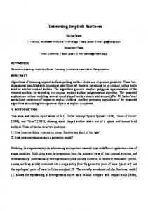
2.4 Trimmed NURBS Geometric modeling of general shapes requires the ability to add holes or to intersect two objects, for example. This is needed because even simple geometries consist of several patches, which are mostly also trimmed ones. The boundaries of such trimmed patches are defined by trimming curves, which, for instance, are the result of applying an edge fillet to smoothen a structure. Figure 2.6 visualizes two NURBS patches intersecting with each other. At the intersection edge an edge fillet is applied. The fillet results in an additional NURBS patch. Please keep in mind that these three patches generally have a different parameterization. Such kinds of geometrical configurations are frequently appearing, e.g., in the design of mechanical parts of an automobile. Of course, there are other methods like Subdivision Surfaces or T-Splines which allow to model a geometric part as one entity. On the other hand, only NURBS allow the designer to model such kind of objects so intuitively at this level of precision. A trimmed NURBS surface is defined as a tensor product with a restricted parametric domain. The restriction comes along with a set of properly ordered trimming curves. Figure 2.7 shows two NURBS patches and trimming curves in the parametric domain. The gray-shaded part of the parametric domain represents the restriction of the parametric domain. This restricted part mapped on the physical space yields a trimmed NURBS surface. A trimming curve, no matter if it is closed or not, divides the parametric domain into two parts. This definition is not sufficient because it cannot be distinguished to which part of the parametric domain this restriction applies. Therefore, a common

2.4 Trimmed NURBS

13

v

v u

u Figure 2.7: Two examples of trimmed NURBS patches shown in the parametric domain.

definition states that the part on the right side along the direction of the trimming curves is void. When the parametric domain is restricted by several trimming curves, only a proper ordering ensures a valid surface. For example, if the direction of the lowest curve on the left plot of Figure 2.7 pointed opposite, it would not be possible to define a surface. Since within this thesis only single trimming curve problems are considered, the corresponding definitions are restricted accordingly in order to simplify the discussion. Let us assume a NURBS surface S(u,t) and a trimming curve C(t), as defined in (2.10) and (2.9), respectively. As stated before, the direction of the curve determines the part being cut off, i.e., the surface domain on the right side of the trimming curve. In order to represent a trimmed surface exactly each curve parameter has to be expressed in terms of the coordinates of the parametric surface. Consequently, the new boundary of the NURBS surfaces SΓ , could be defined as SΓ (u(t), v(t)) =

mv mu

∑ ∑ Ri,j (u(t), v(t)) · Pi,j

(2.20)

j =0 i =0

Since it is not possible to determine for each curve parameter t the corresponding surface parameter pair (u(t), v(t)), a proper restriction of the parameter domain of the underlying NURBS surface is impossible. This matter is one of the big issues when dealing with trimmed surfaces in the context of isogeometric analysis, because the integration domain of the trimmed knot spans cannot be properly defined. All these actions require intersecting and trimming tools to work in conjunction with the underlying basis used for the geometric model. These tools are all based on trimming the underlying NURBS patches, as NURBS are the standard methodology in representing geometric objects. These techniques are not only required in the field of geometric modeling but also in the field of Computer-Aided Manufacturing (CAM), where the intersections of offset surfaces with parallel planes need to be computed in order to generate the paths for 3-D milling machines, see, for example, Lartigue et al. [2001]. As stated in Patrikalakis and Maekawa [2001], the problem of finding intersections is to capture efficiently all features of the solution while keeping up a high precision. Moreover, the employed algorithms have to be highly reliable. For the case of surface to surface intersection, three methods are mainly used, i.e., Lattice methods, Subdivision methods, and

14


Zoom

(a) Two intersected NURBS patches.

(b) Zoomed view on the intersection curve and trimmed edges of the NURBS patches. The red curve is the intersection curve between the two patches. The blue curve is the edge of the left patch obtained by trimming the left patch with the right patch. The green curve is the resulting edge of the left patch by trimming this one with the intersection curve. Figure 2.8: Intersection problem of two NURBS patches.

Marching methods. One of the first publications dealing with intersections of B-Splines was published by Dokken [1985]. For details on finding the intersection of different types of geometries the interested reader is referred to chapter 25 of Farin et al. [2002] or Patrikalakis and Maekawa [2001] and the references therein. After the intersection is determined, the NURBS patch has to be trimmed. In the CAGD community between two kinds of trimming methods is distinguished. The most widespread technology is visual or graphical trimming. Herein, the underlying NURBS patch remains unaltered. Only the visualization is adapted to the new domain. The first publications on this topic can be found in Farouki [1987], Casale [1987], or Crocker and Reinke [1987]. The other methodology is denoted as geometric or mathematical trimming in which the trimmed patch is replaced by a new untrimmed patch. The first publications dealing with this topic are Hoschek [1987], Hoschek [1988], and Hoschek et al. [1989]. The problem of determining the intersection curve between two surfaces is a nontrivial task. Generally, the degree of the intersection curve can be very high. Thus, it is not used in practical applications. In other cases, the degree is even not known, e.g., the intersection between two NURBS surfaces with unequal weights. The common way is to approximate the trimming curve with a sequence of cubic curves. Consequently, the trimming curve is an approximation of the real curve and the involved error leads to a non-matching intersection definition between the patches. In Figure 2.8 two intersected NURBS surfaces are shown. These surfaces are modeled and intersected within Rhino 3D (www.rhino3d.com). In Figure 2.8(b), three different curves are depicted. The red curve represents the intersection of both patches. The blue curve is obtained by trimming the

2.4 Trimmed NURBS

15

left patch with the (red) intersection curve. The green is the results of trimming the left patch with the right patch. Please note that all these curves are the result of applying the corresponding tools within Rhino 3D. Actually, all these curves should be the same. The difference is the result of the approximations. The associated error results in gaps or overlays of the geometric model. Moreover, the modeling sequence has an effect and decides about the quality of the geometrical model. This may render further analysis on the resulting multi-patch difficult if not impossible. Furthermore, this might be the source of incompatibilities, for example, between different CAD software or within a preprocessing tool for a Finite Element software, which cannot create a finite element mesh based on the given geometric model. In Isogeometric Analysis, one is facing the same issue, since the geometry remains unaltered throughout the analysis process. Consequently, a methodology for Isogeometric Analysis on trimmed NURBS surfaces must be capable of handling these deficiencies in a geometric model.

Chapter

3

Basics of mechanics This chapter provides a short description of the structural mechanics problem dealt within this thesis. Moreover, the numerical treatment of the basic equations with the Finite Element Method is briefly delineated. A detailed coverage of this topic is intentionally omitted. The interested reader is referred to the excellent textbooks of Holzapfel [2000]; Mardsen and Hughes [1983]; Parisch [2003]; Stein and Barthold [1997].

3.1 Structural Mechanics This section introduces the description of the kinematics of a structural object. Additionally, the balance laws and the resulting differential equations a structure obeys are presented. For the derivation of the equations the Lagrangian approach is adopted, i.e., the properties of a point in a structure depend on the initial position and time.

3.1.1 Kinematics The path of deformation of a moving body is governed by its kinematics. In general, a distinction is made between the initial position of a body and the state of the same body after some movement which are denoted as reference configuration and current configuration, respectively. A body is defined as an agglomeration of material points in the three-dimensional Euclidean space R3 . The basis of this spatial domain is spanned by a set of orthogonal unit vectors ei . The difference between the material points in the two configurations allows to describe the deformation process. Let us observe a point X in the reference configuration, as shown in Figure 3.1, which is defined by the basis vectors of the Euclidean space and its components or coordinates Xi as X = Xi e i

(3.1)

In the material description, i.e., the Lagrangian description of motion, the position in the current configuration is expressed in terms of the material coordinates, i.e., the components of the material points in the reference configuration, namely x = Φ(X, t)

(3.2)

18

Basics of mechanics

reference configuration

current configuration

at time t = t0

at time t = tn Φ(X, t)

B

Ω0

dX

Ω u

A

A’ dx B’

X

e3

x

e2 e1 Figure 3.1: Configurations of a material body

where Φ(X, t) is a time-dependent mapping of the material points of a body between their reference and current configurations. This allows to formulate the displacement vector as follows u(X, t) = Φ(X, t) − Φ(X, t0 ) = x(X, t) − X

(3.3)

In the following the dependency on time is dropped, because within this thesis only quasi-static deformations are considered. In order to study deformations, let us consider the differential distances dX and dx in the neighborhood of a material point in the reference and current configuration. This setup is depicted in Figure 3.1. The total derivative dx can be written as (see also Stein and Barthold [1997]) dx =

∂x ∂x ∂x ∂x dX 1 + dX 2 + dX 3 = dX ∂X1 ∂X2 ∂X3 ∂X

(3.4)

Defining the deformation gradient F as F :=

∂x ∂X

(3.5)

a linear map between the differential elements in the reference and current configuration is defined as dx = F · dX

(3.6)

It is important to ensure the existence of the inverse mapping of Φ(X, t) in order to guarantee that the material points form a continuous body. This implies that the inverse of the deformation gradient also exists. According to Stein and Barthold [1997], this is satisfied if the determinant of the deformation gradient is nonzero, i.e., det F ̸= 0. To avoid self

3.1 Structural Mechanics

19

penetration in addition, one generally requires det F to be strictly positive, i.e., det F > 0. Generally, the deformation gradient may be used as a strain measure since it measures the state of deformation. However, the deformation gradient is nonzero when applying rigid body motions and is directionally dependent. Thus, other strain measures are employed, see, for example, Stein and Barthold [1997] for further elaboration. A commonly used strain measure is the Green-Lagrange strain tensor E. It is defined as follows E=

) 1( T F ·F−I 2

(3.7)

It is a symmetric second order tensor which results in a zero strain state for arbitrary rigid body motions and is invariant with respect to directions. There are other strain measures, e.g., the Euler-Almansi strain tensor. The corresponding derivations and definitions of these strain measures can be found, for example, in the textbooks of Ogden [1997] and Holzapfel [2000].

3.1.2 Constitutive equation The relation between strains and stresses is given by the so-called constitutive equations via a material law. The field of constitutive models is a very broad field, see, for example, Holzapfel [2000]. Within this thesis, only linear elastic materials are considered. Thus, the stress state of these materials does depend just on the actual strain state. Additionally, assuming that the deformation history has no influence, the material can be characterized as hyperelastic. This allows to formulate a strain energy function or elastic potential W, see, for example, Parisch [2003]. In the reference configuration, this potential depends on the second Piola-Kirchhoff stress tensor S and the Green-Lagrange strain tensor E. In particular, the stress tensor can be defined as follows (see also Parisch [2003]) S(E) =

∂W(E) ∂E

(3.8)

The derivative of the stress tensor with respect to the strain tensor yields the material tensor which reads as follows C=

∂S ∂2 W( E ) = ∂E ∂E2

(3.9)

Within this thesis it is assumed that only small strains are occuring. This allows to use a St. Venant Kirchhoff material law. This material law defines a linear relation between the strains and the stresses, i.e., S=C:E

(3.10)

Please note that no restrictions are made concerning the deformations. More information and details about constitutive equations and their formulations can be found, for example, in the textbooks of Ogden [1997] and Simo and Hughes [1998].

3.1.3 Boundary Value Problem Within this thesis, structural mechanical problems are being considered. The related equations can be derived based on continuum mechanical considerations. The partial

20

Basics of mechanics

differential equations of the static structural mechanical problem, i.e., the local momentum equation, can be stated in the reference configuration as div (F · S) + ρ0 · B = 0

in Ω0

(3.11)

where ρ and B are the density and body forces acting within the computational domain Ω0 . Generally, this partial differential equation is formulated in the current configuration. For the transformation to the given form, the reader is referred to Mardsen and Hughes [1983] or Parisch [2003]. Additionally, these equations are supplemented with the boundary conditions u = u0 in ΓD F·S·n = t

(3.12)

in ΓN

(3.13)

where ΓD and ΓN denote the Dirichlet and Neumann part of the boundary of the domain. t is a traction applied on the Neumann boundary and u0 are prescribed displacements at the Dirichlet boundary. The combination of the kinematics, the constitutive law, and the given partial differential equations forms the strong form of the Boundary Value Problem of Elastostatics.

3.2 The Finite Element Method The most applied and wide-spread numerical method to obtain an approximate solution of a partial differential equation is the Finite Element Method. It is based on variational methods which allow to transform the differential equation into an integral expression. Consequently, a point-wise satisfaction of the equations is not required. The advantage of this concept is that simpler functions can be employed to seek for the solution. Thus, it allows for the solution of partial differential equations where the actual solution cannot be identified analytically. The mathematical background of the Finite Element Method can be found in Brenner and Scott [2008]. More engineering-related literature is given, for example, in the textbooks of Bathe [2002], Hughes [2000], and Zienkiewicz et al. [2005].

3.2.1 Weak Form In order to solve the structural mechanics problem, as presented in section 3.1.3, with the help of the Finite Element Method, (3.11) is multiplied with a test function δu. This test function has to obey several properties: • satisfies the geometric boundary conditions: δu = 0 on ΓD • is arbitrary and infinitesimal small In addition to the multiplication with the test function and subsequent integration over the domain, the Gauss Integration Theorem is also employed. This yields the following integral equation: ∫ Ω0

∇δu : (F · S) dΩ =

∫ Ω0

δu · ρ0 · B dΩ +

∫ ΓN

δu · t dΓ

(3.14)

3.2 The Finite Element Method

21

Using the identities δF = and

∂ δ (X + u) = ∇δu ∂X

(3.15)

( ( )) 1 T δE : S = δ F ·F−I :S 2 ) 1( T δF · F − δF · FT : S = 2 = δFT · F : S

(3.16) (3.17) (3.18)

= δF : (F · S) = ∇δu : (F · S)

(3.19) (3.20)

the momentum equation in (3.14) can be rewritten in terms of the Green-Lagrange strain tensor: ∫

δE : S dΩ =

Ω0

∫

δu · ρ0 · B dΩ +

Ω0

∫

δu · t dΓ

(3.21)

ΓN

These equations represent the weak form of the Boundary Value Problem, as given in section 3.1.3. Since the individual terms in (3.21) represent work expressions, it is also referred to as the Principle of Virtual Work. There are other approaches which use in addition to the displacements also strains and stresses as free variables, e.g., the Hellinger-Reissner principle and the Hu-Washizu principle. Please refer to Washizu [1975] for details. The term on the left side of (3.21) is denoted as the internal virtual energy δWint . The expression on the right side is defined as the external virtual energy δWext . From (3.21) it can be observed that the sum of internal and external virtual work vanishes for any admissible virtual displacement. This in turn means that the system is in equilibrium and that the variation of the energy in the system vanishes, i.e., δW = δWint + δWext = 0

(3.22)

3.2.2 Discretization In terms of the Finite Element Method, the computational domain Ω is decomposed in a finite set of n elements, i.e., h

Ω≈Ω =

n ∪

h

Ωe

(3.23)

e =1

Consequently, an approximation of the original domain is obtained, i.e., Ωh . Moreover, this domain is defined such that the individual elements do not overlap. The discrete boundary of the domain consists of the curves or surfaces of the m elements at the boundary. This can be written as ∂Ω ≈ ∂Ωh =

m ∪

∂Ωrh

(3.24)

r =1

In general, the discrete boundary represents also only an approximation to the real boundary of Ω.

22

Basics of mechanics

These approximation errors depend on the number and the type of elements used. Often, only linear elements are employed. This results in a large approximation error, especially in curved regions. Thus, the number of elements must be increased to counter balance this effect. Please note that there are functions which can avoid these geometric approximation errors, see chapter 4 for details. Commonly, the same functions are being used for discretization of the geometry and the field variables in the Finite Element Method. This concept is known as the Isoparametric Concept. In particular, the geometry in reference and current configuration can be defined as a geometric map from a parameter domain Ω onto the computational domain, i.e., h and g : Ω → Ω h Ge : Ω → Ωe,0 e e Ge ( ξ ) : = X ( ξ ) =

k

∑ Na (ξ ) Xˆ a

(3.25)

a =1

ge ( ξ ) : = x ( ξ ) =

k

∑ Na (ξ ) xˆ a

(3.26)

a =1

ˆ a and xˆ a are coefficients defining the geometry in the reference and current The terms X configuration. Within (3.25)-(3.26), Na (ξ ) are shape functions, usually polynomials, defined in the parameter domain Ω . The field quantities, i.e., the displacements, can be expressed in the following form k

u (X) =

∑ Na

a =1

k

u (x) =

∑ Na

( (

) 1 G− X uˆ a ( ) e

(3.27)

) 1 G− x uˆ a ( ) e

(3.28)

a =1

The term uˆ a represents the control variables of the field quantity and are located at the points defining the geometry. Decomposing (3.21) with the definitions (3.23) and (3.24), one obtains the following integral equation for a single element: ∫

δE : S dΩ =

h Ωe,0

∫

δu · ρ0 · B dΩ +

h Ωe,0

∫

δu · t dΓ

(3.29)

h Γe,N

Using the definition of the variation of the Green-Lagrange strain tensor δE =

∂E δu a ∂u a

(3.30)

the discrete form of (3.29) can be rewritten as follows k

∑

a =1

δuˆ a

∫ h Ωe,0

∂E : S dΩ = ∂u a

k

∑

a =1

δuˆ a

∫ h Ωe,0

Na · ρ0 · B dΩ +

k

∑

a =1

δuˆ a

∫ h Γe,N

Na · t dΓ

(3.31)

3.2 The Finite Element Method

23

Introducing the following definitions for the internal and the external force vector Re,int a

∫

:= h Ωe,0

Re,ext := a

∫

∂E : S dΩ ∂u a Na · ρ0 · B dΩ +

h Ωe,0

(3.32) ∫

Na · t dΓ

(3.33)

h Γe,N

allows to formulate the equilibrium of forces in matrix notation as: δuˆ T Rint = δuˆ T Rext

(3.34)

Employing the definitions of the variations and rearranging (3.34) one obtains Rint − Rext = 0

(3.35)

Please note that the internal force vector depends on the state variables, i.e., Rint = Rint (uˆ ). In general, it is a nonlinear function of the state. Therefore, the nonlinear equation (3.35) has to be solved in an iterative way. A common approach is to use a Newton-Raphson scheme, see Hanke-Bourgeois [2009] for details. This method requires a linearization of (3.35) with respect to the state variables. This results in the following linear equation system, which has to be solved at each iteration step, namely ( ) ( ) ∂ Rint (uˆ ) − Rext ∆u = − Rint (uˆ ) − Rext (3.36) ∂u where ∆u describes the difference of state variables between two iteration steps. Commonly, the derivative of the force vectors with respect to the state variables is denoted as tangent stiffness matrix: ( ) ∂ Rint (uˆ ) − Rext Kt := (3.37) ∂u In case no path-dependent loadings are considered, the tangent stiffness matrix is independent from the external load vector. For details about linearizations of the internal force vector the interested reader is referred to the textbooks of Wriggers [2001]; Parisch [2003].

Chapter

4

Isogeometric Analysis Isogeometric Analysis is a recent technology in the Finite Element Analysis world. The benefits of this methodology are recognized by many researchers around the world. This is reflected in the vast amount of publications which appeared in the last couple of years. The list of applications and associated publications of Isogeometric Analysis is already too huge to list them all, so only some selected publications are given exemplarily: • Origin: Hughes et al. [2005]; Bazilevs et al. [2006a]; Cottrell et al. [2006, 2007] • Finite Element Technology: Auricchio et al. [2010b,a]; Echter and Bischoff [2010]; Hughes et al. [2010]; Vuong et al. [2011] • Structural Mechanics: Benson et al. [2010]; Dornisch et al. [2013]; Echter et al. [2013]; Elguedj et al. [2008]; Kiendl et al. [2009]; Temizer et al. [2011] • Fluid Mechanics: Bazilevs et al. [2007]; Bazilevs and Hughes [2007, 2008] • Multi-Physics: Bazilevs et al. [2006b, 2008]; Bazilevs and Hughes [2008]; Bazilevs et al. [2011a,b] • Optimization: Nagy et al. [2010a, 2011]; Seo et al. [2010a,b]; Wall et al. [2008] • other Splines: Burkhart et al. [2010]; Cirak et al. [2002]; Dörfel et al. [2010]; NguyenThanh et al. [2011] This chapter provides a general introduction to NURBS-based Isogeometric Analysis, i.e., what are its properties, differences and common features to the standard Finite Element Method. In addition, the applied finite element formulation, i.e., a Kirchhoff-Love shell element, is concisely delineated.

4.1 Attributes As the term Isogeometric Analysis implies, an analysis is performed where the geometric model and the analysis model are the same, i.e., iso. Consequently, the geometric discretization error is excluded ab initio, which can be written as Ω=Ω

h

∂Ω = ∂Ω

h

(4.1) (4.2)

26

Isogeometric Analysis

CAD

Standard FEM spline basis


Design Model spline basis

Meshing

CAE

polynomial basis

Analysis Model

isoparametric (polynomial basis)

isoparametric (spline basis)

Geometric Model

Geometric Model

Solution Field

Solution Field

Figure 4.1: Comparison of standard Finite Element Method and Isogeometric Analysis.

This is a substantial improvement compared to the standard finite element method, confer (3.23) and (3.24). Moreover, the analysis model and the solution field are expressed in the same basis. This is commonly known as the isoparametric concept. The hierarchy and the connection of these models are highlighted and compared to the standard finite element method in Figure 4.1. The most apparent feature of Isogeometric Analysis is its inherent nature of integrating design and analysis. For instance, no conversion between the models used in design and analysis is required since they share already the same basis. The process of generating a finite element mesh is generally very time consuming, confer, for example, Figure 1.2 in Cottrell et al. [2009]. Thus, this represents a huge improvement compared to standard FEM. Moreover, less control variables are required for the same approximation power using NURBS basis functions compared to their standard FEM counterparts. This fact is exemplarily highlighted for quadratic basis functions of NURBS and Lagrange polynomials in Figure 4.2. In particular, a 1D NURBS patch of degree p with n elements and a knot multiplicity of m has ( p + 1) + (n − 1) · m control variables. The Lagrange counterpart requires p · n + 1 control variables. Thus, the size of the equation system with NURBS elements is smaller than the one with Lagrange elements, especially for many elements. Consequently, NURBS-based Isogeometric Analysis is computationally more efficient from a per-degree-of-freedom point of view. These properties can be attributed to the high continuity across element boundaries with a NURBS patch. The reason of these properties emanates from the powerful basis of the NURBS. An important characteristic of this methodology is the simplification of the refinement process. In particular, adding control variables and increasing the approximation order can be performed without altering the geometric model. This results in an easy and fast adaptation of the simulation

4.1 Attributes

27 1 0.8 0.6 0.4 0.2 0

0

0.25

0.5

0.75

1

0.75

1

(a) Quadratic B-Spline functions.

1 0.8 0.6 0.4 0.2 0 -0.2 0

0.25

0.5

(b) Quadratic Lagrange polynomials.

Figure 4.2: Comparison of quadratic B-Splines and Lagrange polynomials for a model consisting of four elements.

model according to the underlying physics. On the contrary, applying the standard finite element method, a repeated sequence of mesh generation would be required which is very time consuming. Moreover, it is not possible to distinguish if refinement is necessary because of insufficient geometric representation or lack of approximation power. Therefore, Isogeometric Analysis is an attractive method for the analysis of large systems. A drawback of Isogeometric Analysis is the non-interpolatory nature of the control variables of a NURBS patch rendering the application of Dirichlet conditions difficult. Therefore, enforcing arbitrary Dirichlet conditions in a weak sense is demanded. For instance, a weak enforcement of Dirichlet conditions was successfully applied in Bazilevs and Hughes [2007] and Embar et al. [2010]. Although Dirichlet conditions cannot be applied straightforwardly, the exact boundary description, confer (4.2), in Isogeometric Analysis is advantageous compared to the approximate boundary in standard FEM, check (3.24).

28


4.2 Element definition and Integration In general, a set of NURBS patches comprises the computational domain. The nonzero knot spans of these NURBS patches are identified as finite elements. Within each NURBS patch, the continuity properties are inherited because the elements are the image of the geometric map from the parametric domain of the NURBS basis functions. In particular, the continuity across element boundaries within a NURBS patch is Cp−m , where p and m are the polynomial degree and the multiplicity of a knot, respectively. This is a clear distinction to the standard Finite Element Method, where the highest achievable inter element continuity is typically C0 -continuity. Figure 4.3 depicts a NURBS patch in the physical and parametric domain. A knot span or finite element is highlighted in the respective domains. Additionally, the integration domain is visualized. Whereas the map between the integration domain and the parametric domain is a linear map, the geometric map from the parametric domain onto the physical space is generally nonlinear. The control points of a NURBS patch are employed as control variables in the analysis. Thus, the control variables of an element are the ones whose basis functions are nonzero within the respective knot span. The structure of the control net proposes an ordering of the control variables which is used within the analysis. The fact that NURBS control points are not interpolating the geometry does not yield an issue. The reason is that the NURBS basis fulfills all requirements for a Finite Element Analysis. They can be summarized as: • partition of unity • linear independence • compact support • affine covariance The integration of each finite element is performed knot span wise. Within each knot span the basis functions are C ∞ . Thus, standard integration schemes, e.g., Gauss integration, can be used. An important consequence of this element-wise integration scheme is that the basis functions are over-integrated since the inter-element continuity is not considered. Consequently, this integration scheme renders Isogeometric Analysis non-optimal in terms of computational efficiency. In Hughes et al. [2010] a study was initiated with the aim to develop an integration scheme suited for Isogeometric Analysis. In Auricchio et al. [2012] this research is continued. Although this contribution extended the range of applicability of the integration scheme, the proposed scheme is not applicable to arbitrary parameterizations of a patch. Thus, Gaussian quadrature, despite its inefficiency, is applied in an element-wise fashion within this thesis.

4.3 Refinement In Isogeometric Analysis, the refinement of the analysis model is performed by employing the tools provided from CAGD. Generally, it is possible to increase the density of knots and the polynomial degree of a NURBS patch. Since refinement methods are developed for B-Spline patches, the refinement of a NURBS patch is applied to its homogeneous form, where a NURBS patch reduces to a B-Spline patch. Interestingly, both refinement processes do not change the geometry neither geometrically nor parametrically. Mesh refinement is performed by increasing the number of knots. This is denoted as Knot

29

Physical Space

4.3 Refinement

Parametric Space

v

Integration Domain

u η

ξ

Figure 4.3: Definition of elements and the integration domain in Isogeometric Analysis, compare Cottrell et al. [2009]. The continuous black lines represent the knots, i.e., the element boundaries. In the top picture the red dashed lines and the red framed white points represent the control net of the NURBS surface.

30


Refinement. The new knots divide the existing knot spans into smaller ones and introduce new basis functions, confer (2.2) and (2.3). Accordingly, the number of control points of the B-Spline patch is increased as well. The new control points are obtained as linear combinations of the existing control points by applying the de Casteljau algorithm. Degree Elevation denotes the approach to increase the polynomial degree of a patch. Elevating the degree of a patch comes along with adding a control point to the control net. The general procedure is to represent the patch in its Bézier form and to increase the polynomial degree with available algorithms. The degree elevated B-Spline patch is obtained by removing internal knots until the continuity at the knots equals the one before the degree elevation.

4.4 Element formulation The basis for the Isogeometric Analysis of thin-walled structures performed within this thesis is the Kirchhoff-Love shell element, as proposed in Kiendl et al. [2009]. This section provides a concise overview of this element formulation. The interested reader is referred to Kiendl et al. [2009] or to Kiendl [2011] for more details.

4.4.1 Assumptions The Kirchhoff-Love shell theory postulates that cross sections remain straight and normal to the mid-surface of the shell body independent of the deformation state. Consequently, the effect of transverse shear deformations is excluded. This assumption restricts the validity of this shell element to thin-walled structures. In particular, the slenderness of a shell, i.e., the ratio between the radius of curvature and the thickness of the shell, has to be larger than twenty. Furthermore, it is assumed that the thickness of the shell remains unaltered during deformation, i.e., transverse normal strains can be excluded.

4.4.2 Kinematics A point in the shell body is described by the position vector P of the shell mid-surface and a director D into the shell’s body. Consequently, a material point can be written in reference and current configuration, respectively, as follows (see also Bischoff et al. [2004]) ( ) ( ) ( ) X θ1, θ2, θ3 = P θ1, θ2 + θ3 D θ1, θ2 ( ) ( ) ( ) 1 2 3 1 2 3 1 2 x θ ,θ ,θ = p θ ,θ +θ d θ ,θ

(4.3) (4.4)

where θ i are the parameter coordinates describing the shell’s body. Moreover, p and d denote the position vector and the director in the current configuration. The displacement is described by the difference of the material points, i.e., u = x − X = p − P + θ 3 (d − D)

(4.5)

4.4 Element formulation

31

The requirement that the director has to be orthogonal to the mid-surface is satisfied by constructing the director as the normalized cross product of the mid-surface base vectors. The base vectors of the mid-surface are defined as follows: ( ) ∂X θ 1 , θ 2 , 0 ∂P Aα = = α = P,α (4.6) α ∂θ ( ∂θ ) ∂x θ 1 , θ 2 , 0 ∂p ∂P + u aα = = α = p,α = = Aα + u,α (4.7) ∂θ α ∂θ ∂θ α A1 × A2 = A3 ∥ A1 × A2 ∥ a1 × a2 d= = a3 ∥ a1 × a2 ∥

(4.8)

D=

(4.9)

This definition allows to define the base vectors at an arbitrary point in the shell body as ( ) ∂ P + θ 3 A3 ∂X Gα = α = = Aα + θ 3 A3,α (4.10) α ∂θ ∂θ ( ) ∂ p + θ 3 a3 ∂x gα = α = = aα + θ 3 a3,α (4.11) ∂θ ∂θ α Based on the assumptions in section 4.4.1, only the coefficients of the mid-surface enter the definition of the Green-Lagrange strain tensor E. Consequently, the coefficients of the strain tensor (3.7) are given by Eαβ =

) 1( gαβ − Gαβ 2

(4.12)

Computing the metric coefficients Gαβ and gαβ with their definitions as given in (4.10) and (4.11) and inserting them into (4.12) one obtains: Eαβ =

) ( )2 ( 1( aαβ + θ 3 aα · a3,β + a β · a3,α + θ 3 aα · a3,β 2 ) ( ) ( )2 − Aαβ − θ 3 Aα · A3,β + A β · A3,α − θ 3 Aα · A3,β

(4.13)

Assuming a thin shell, it is a valid assumption to neglect the quadratic terms in (4.13), confer Bischoff et al. [2004]. Moreover, recalling the definition of the second fundamental form, see Klingbeil [1989], which defines the curvature tensor at a point on a surface, i.e., ) 1( Aα · A3,β + A β · A3,α 2 ) 1( = − aα · a3,β + a β · a3,α 2

Bαβ = −Aα · A3,β = −A β · A3,α = −

(4.14)

bαβ = −aα · a3,β = −a β · a3,α

(4.15)

the coefficients of the Green-Lagrange stain tensor can be rewritten as Eαβ =

) ( ) 1( aαβ − Aαβ + θ 3 Bαβ − bαβ 2

(4.16)

This shows that the strain coefficients do only depend on the displacements of the midsurface, i.e., uα . The first term on the right side of (4.16) is related to membrane action, because the difference between the metrics of the mid-surface is measured. The other term describes the

32


difference in the curvatures. Therefore, is is related to bending. With the definition of membrane strains and changes in curvature by ε and κ, respectively, one obtains Eαβ = ϵαβ + θ 3 καβ

(4.17)

Due to the assumptions made in section 4.4.1, it is possible to analytically pre-integrate the material tensor over the thickness, see Bischoff et al. [2004] for details. In analogy to membrane strains and changes in curvature, normal forces n and bending moments m can be defined as follows: n = Dn : ε

(4.18)

m = Dm : κ

(4.19)

where Dn and Dm are the material tensors related to the normal strains and changes in curvature, respectively.

4.4.3 FE-equations With the previous definitions of strains and stresses for a Kirchhoff-Love shell element, the related internal and external virtual work expression can be formulated as follows: ∫

δε : n + δκ : m dΩ =

A0

∫

δu · ρ0 · b dΩ +

∫

δu · t dΓ

(4.20)

Γ0

A0

Discretization and linearization of (4.20) provides the internal and external forces as well as the tangent stiffness matrix, i.e., ) ∫ ( ∂κ ∂ε e,int : n+ : m dΩ Ra = (4.21) ∂u a ∂u a A0

Re,ext a

∫

= A0

Ke,int ab

Na · ρ0 · b dΩ +

∫ (

= A0

∫

Na · t dΓ

Γ0

∂2 ε ∂ε ∂n ∂2 κ ∂κ ∂m : n+ : + : m+ : ∂u a ∂ub ∂u a ∂ub ∂u a ∂ub ∂u a ∂ub

(4.22) ) dΩ

(4.23)

For a detailed derivation of the FE equations, the interested reader is referred to Kiendl [2011].

Chapter

5

Coupling of nonconforming discretizations This chapter introduces several possibilities to couple nonconforming discretizations of NURBS-based geometric entities. Moreover, it serves as a basic investigation for later developments. After the theoretical basics are delineated, possibilities to project field and flux quantities are described. The methods are investigated for mapping quantities on a flat and a curved interface considering different combinations of polynomial degrees.

5.1 Coupling methods This section discusses the theoretical background of coupling methods. The methods comprise an Interpolation Method, a Least-Squares Method, and a Weighted-Residual Method. The general task of coupling methods is to represent an arbitrary function f in terms of a given function g. Let us assume the given function can be represented as a linear combination of basis functions and their coefficients. Consequently, the problem can be formulated as n

g(u) =

∑ Ni (u) · Pi

(5.1)

i =1

g(u) − f = 0

∀u

(5.2)

where Ni and Pi are basis functions and coefficients of the given function g.

5.1.1 Interpolation Method Task of interpolation is to find the coefficients of a given function g such that the target function f and g agree at least at some points, denoted as interpolation or sampling points. It is obvious that the location of the sampling points can have a big effect on the approximation properties of the function g. The general interpolation task can be stated as n

∑ Ni (uk ) · Pi − f k = 0

i =1

for k = 1, · · · , a

(5.3)

34

Coupling of nonconforming discretizations

where uk denotes the parametric value of a sampling point k and f k represents the value of the target function at sampling point k. Moreover, "a" denotes the number of sampling points. Assuming an arbitrary parameterization of the target function f , (5.3) can be rewritten as n

m

i =1

j =1

∑ Ni (uk ) · Pi − ∑ Mj (vk ) · Fj = 0

for k = 1, · · · , a

(5.4)

where M j and Fj are the basis functions and coefficient of the target function f . In matrix notation, (5.4) reads as follows NP − MF = 0

(5.5)

Solving (5.5) for the unknowns P, provides the coefficients of the function g for which function f is interpolated at the selected sampling points. It is necessary that the number of sampling points and the number of coefficients of g are the same, i.e., a = n. Otherwise (5.5) is not solvable. Additionally, a transformation matrix T between the coefficients of both functions can be defined by T = N −1 M

(5.6)

5.1.2 Discrete Least-Squares Method The point of departure for the discrete Least-Squares Method is (5.2). The target is to minimize the error E of the squared differences between two functions g and f , namely E = ( g − f )2

(5.7)

It is known that the error of this problem is minimal when the partial derivatives of the error with respect to the coefficients of functions g vanish. The derivatives can be formulated as ( )2 n m ∂E ∂ (5.8) = Ni (uk ) · Pi − ∑ M j (vk ) · Fj ∂Pl ∂Pl i∑ =1 j =1 ( )

= 2Nl (uk )

n

m

i =1

j =1

∑ Ni (uk ) · Pi − ∑ Mj (vk ) · Fj

for l = 1, . . . , n

(5.9)

Setting each of the equations in (5.9) to zero yields the following linear equation system n

n

n

m

l =1

i =1

l =1

j =1

∑ Nl (uk ) ∑ Ni (uk ) · Pi − ∑ Nl (uk ) ∑ Mj (vk ) · Fj = 0

(5.10)

The matrix form of (5.10) reads as follows NT NP − NT MF = 0

(5.11)

Comparing (5.11) with (5.5), one can observe that the discrete Least-Squares Method can be obtained by multiplying the equation of the Interpolation Method with the transpose of the shape function matrix of function g. In contrast to the Interpolation Method, the Least-Squares Method allows to have more sampling points than number of unknowns. In particular, the number of sampling points have to big enough in order to obtain a good approximation, see, for example, Farin et al. [2002]. The transformation matrix between the coefficients of the two functions is given by ( ) −1 T = NT N NT M (5.12)

5.1 Coupling methods

35

5.1.3 Weighted-Residual Method Another method to approximate f with a given function g is a Weighted-Residual Method. This method minimizes the integral of a weighted difference to the given functions. Firstly, (5.2) is multiplied with a weighting function w. The next step is to integrate the resulting product over their domain of definition. Thus, (5.2) is transformed to ∫

w · ( g − f ) dΩ = 0

(5.13)

Ω

Introducing a discretization of the respective functions and the weighting function into (5.13), one obtains ( ) ∫ a

∑ Wl · wbl ·

∫

Ω l =1

(

a

∑ wbl ·

Wl

Ω l =1

n

m

i =1

j =1

∑ Ni (u) · Pi − ∑ Mj (v) · Fj

n

m

i =1

j =1

dΩ = 0

(5.14)

dΩ = 0

(5.15)

)

∑ Ni (u) · Pi − Wl ∑ Mj (v) · Fj

b is the pair of basis function and coefficient of the weighting function w. where (W, w) A property of the weighting function and its coefficients is that they are arbitrary and non-zero. The fundamental lemma of variational calculus, states that (5.15) can only be fulfilled if the term in the brackets within the integral expression vanishes. Consequently, this expression minimizes the difference between the two functions. From (5.15) the following linear equation system can be identified a

n

∑∑

∫

l =1 i =1 Ω

a

Wl · Ni (u) dΩ · Pi − ∑

m

∑

∫

Wl · M j (v) dΩ · Fj = 0

(5.16)

l =1 j =1 Ω

Grouping the individual integral expressions of (5.16) into the matrices ∫

Al,i :=

Wl · Ni (u) dΩ

(5.17)

Wl · M j (v) dΩ

(5.18)

Ω

∫

Bl,j := Ω

one can rewrite (5.16) in matrix form AP = BF

(5.19)

To render the equation system in (5.19) solvable, the number of weighting functions and functions used for discretizing function g have to be equal, i.e., a = n. A suitable choice for the weighting function is to choose them to be equal to function g, i.e., Wl = Na (u). This specific choice for W is commonly denoted Galerkin Method. Consequently, A becomes a square and symmetric matrix. Matrix B is denoted as projection matrix which projects the discrete function f onto the discrete space of g. Solving (5.19) for the unknown coefficients P provides a transformation matrix T, defined as T = A −1 B which links the discrete function values of g and f .

(5.20)

36


5.2 Field approximation The representation of field data, e.g., displacements, in terms of a known basis provides the corresponding data at any point within the domain with the aid of a finite set of coefficients. Contrary, there are data fields like stresses or tractions which are not explicit functions of basis functions and coefficients. This leads, for example, to difficulties in the post-processing. An option to formulate these kind of fields as linear combinations of basis functions and coefficients is to employ the Galerkin Method, confer, for example, Löhner [2008]. Let us assume a traction field t given on the Neumann boundary. The aim is to represent this field in the following way n

t(u) =

∑ Ni (u) · tî

(5.21)

i =1

where Ni and tî are basis functions and coefficients of the underlying discretization. Applying the Galerkin Method, the error between the given traction field and the chosen parameterization is minimized. Defining the point-wise error as n

ϵ = t(u) − ∑ Ni (u) · tî

(5.22)

i =1

Multiplying (5.22) with Nj as weighting function, integrating over the domain and setting it to zero yields ∫

Nj · ϵ dΩ =

Ω

∫

( Nj ·

n

t(u) − ∑ Ni (u) · tî

) dΩ = 0

(5.23)

i =1

Ω

Rearranging the individual terms results in the following linear equation system n ∫

∑

Nj (u) · Ni (u) dΩ · tî =

i =1 Ω

∫

Nj (u) · t(u) dΩ

for

j = 1, . . . , n

(5.24)

Ω

Using the definitions ∫

A ji :=

Nj (u) · Ni (u) dΩ

(5.25)

Nj (u) · t(u) dΩ

(5.26)

Ω

∫

Bj := Ω

the coefficients tî are obtained by solving the following equation system A ji · tî = Bj

for

i = j = 1, . . . , n

(5.27)

Please note that the expression in definition (5.26) equals the one used for the computation of the consistent nodal force vector. For instance, this procedure can be applied analogously expressing a given stress field in terms of the underlying control variables.

5.3 Mapping quantities

37

5.3 Mapping quantities In coupling non-matching discretizations, it is necessary to distinguish different types of quantities. For instance, in domain decomposition problems it is required to ensure Dirichlet and Neumann boundary conditions at the interface. The reason is that in the FE-equations field quantities, e.g., displacements, and flux quantities, e.g., forces, are present. In order to preserve energy at the interface between two patches, an independent treatment of the individual terms is not admissible. The mapping of displacement fields and forces obtained from a traction field are described in the following.

5.3.1 State mapping Mapping the state, e.g., displacements, from one discretization to another is required to ensure the Dirichlet conditions at the common boundary. In case of a matching discretization at the interface, a point-wise fulfillment of the Dirichlet constraint can be achieved. When the interface is parameterized differently on both sides the Dirichlet condition cannot be satisfied at every point on the interface. To project properly the displacements from one patch to another one, the suitable methods as shown in section 5.1 are employed. In particular, the task is to fulfill the following conditions ua (s, t) = ub (s, t) n

n

i =1

j =1

at ΓSa,b

∑ Ni (s, t) · uˆ ai = ∑ Mj (s, t) · uˆ bj

(5.28) (5.29)

The coupling methods provide a transformation matrix to couple the discrete nodal values of patch A and patch B, namely uˆ ai = Tij · uˆ bi

(5.30)

5.3.2 Force mapping A favorable property at the interface of two distinct discretizations is that no energy is lost or gained. This kind of energy, denoted as interface energy, can be defined as δWinterface =

∫

δu · t dΓ = 0

(5.31)

ΓSa,b

Splitting this equation into the individual components from the two parameterizations, leads to a b δWinterface = δWinterface + δWinterface =0

(5.32)

where a and b are indexes to distinguish between the two sides. Inserting the definitions into (5.32), one obtains ∫ Γ

δua · ta dΓ +

∫ Γ

δub · tb dΓ = 0

(5.33)

38


The state mapping provides us with the relation between the two discrete state variables n

n

m

i =1

i =1

j =1

∑ Ni · uˆ ai = ∑ Ni · ∑ Tij · uˆ bj

ua =

(5.34)

m

ub =

∑ Mj · uˆ bj

(5.35)

j =1

where Tij are the components of the transformation matrix T, as defined in (5.20). The same holds also for the variations of the state variables, i.e., δua =

n

∑ Ni · δuˆ ai =

i =1

δub =

n

m

i =1

j =1

∑ Ni · ∑ Tij · δuˆ bj

(5.36)

m

∑ Mj · δuˆ bj

(5.37)

j =1

Inserting the discrete variations of δu a and δub into (5.33) n m

∑

∑ δuˆ bj · Tji ·

i =1 j =1

∫

m

Ni · ta dΓ + ∑ δuˆ bj · j =1

Γ

n

j =1

i =1

∑ δuˆ bj ·  ∑ Tji ·

∫ Γ

Ni · ta dΓ +

∫

M j · tb dΓ = 0

(5.38)

Γ

Rearranging the terms in (5.38) leads to  m

∫

 M j · tb dΓ = 0

(5.39)

Γ

Using the definition of the individual consistent nodal force vectors Fia :=

∫

Ni · ta dΓ

(5.40)

M j · tb dΓ

(5.41)

Γ

Fjb :=

∫ Γ

and the fact that the terms in the brackets of (5.39) have to vanish, one obtains the following equation system Tji · Fia + Fjb = 0

(5.42)

This equations states that the sum of forces at the interface have to vanish. Thus, this represents the discrete version of the force equilibrium at the interface and provides a computational rule to map the force vector from one mesh to another.

5.4 Numerical investigations The properties of the methods, as introduced in section 5.1, are investigated. These methods are discussed on two different geometric models, i.e., a straight and a curved interface. The properties of the coupling methods are evaluated by mapping several fields (constant, quadratic, and a combination of sine and cosine). Moreover, the influence of

5.4 Numerical investigations

39

(a) Straight interface with equal control point weights. (b) Curved interface with unequal control point weights. Figure 5.1: Geometric models used for testing the mapping methods. The geometric data of these patches can be found in appendix A.

(a) quadratic function

(b) sine and cosine function

Figure 5.2: Fields used for testing the mapping methods.

different polynomial degrees and inter-element continuities are studied. Two geometric models are used throughout the subsequent studies and are depicted in Figure 5.1. The first model is a flat geometry with a linear parameterization. Thus, integration errors regarding the geometry are eliminated. The second model is a curved geometry with varying curvature. This is achieved by setting the weights of the control points unequally. This geometrical model can be seen as a representative of the usual models appearing in isogeometric shell analysis. The geometric data of both models are provided in appendices A.1 and A.2. For each of the two geometric models two different parameterizations are derived and denoted as patch A and B. Thus, the mapping is performed based on geometrically equivalent models. The different fields contained in this discussion are defined as functions of the parameter coordinates u and v. The individual functions f(u, v) are defined as • constant function: f(u, v) = 1 • quadratic function: f(u, v) = u2 + v2 + 2 • sine and cosine function: f(u, v) = sin(u · π ) · cos(v · π ) + 2 Plots of the quadratic and sine and cosine function are provided in Figure 5.2.

40


5.4.1 State mapping The objective of this study is to map the fields, as defined above, from patch B onto patch A for both geometric models. Firstly, the individual fields are discretized in terms of the parameterization of patch B by applying the weighted residual method, confer section 5.2 for details. The resulting discrete data field fB h (u, v ) is projected in a subsequent step A onto patch A to obtain fh (u, v). The following parameterization sets are chosen for the two patches: • polynomial degree: pα = qα = 2, . . . , 4 for α = A, B • number of nonzero knot spans on patch A: (4 × 4), (8 × 8), (16 × 16), (24 × 24), (32 × 32) • number of nonzero knot spans on patch B: (11 × 11) • number of integration points used per nonzero knot span: 5×5 The error in mapping the field data from patch B onto patch A is measured in a relative L2 -norm, namely

A

fh (u, v) − f(u, v) L2 (5.43) estate = ∥f(u, v)∥L2 Mapping a constant function In a first test case, a constant function is mapped from patch B onto patch A. For both geometric models, the mapping error in the L2 -norm is shown in Figure 5.3 for a bi-quadratic patch B. As one can observe, the discrete Least-Squares method and the Weighted Residual method project the constant function independent of the combination of polynomial degrees numerically exact onto patch A. The Interpolation method performs equally well when the density of patch A does not exceed the one from patch B. The combination of a high polynomial degree and a high density of patch A leads to an increase in the mapping error. This error is related to the basis functions in the first and last knot spans of a patch. In particular, there is at least one basis function whose value is orders of magnitudes smaller than the other ones at a sampling point within one of these knot spans. This effect is amplified for high polynomial degrees. These differences introduce numerical errors into the transformation matrix of the Interpolation Method. Consequently, they are responsible for the increase of the error. The same behavior is also observed for a bi-cubic or bi-quartic patch B. Mapping a quadratic function In this test a quadratic function, as depicted in Figure 5.2(a), is mapped from patch B onto patch A. The evolution of the error for the straight interface is visualized in Figure 5.4. As in the previous test case, the function is mapped numerically exact onto patch A for the discrete Least-squares method and the Weighted Residual method. Moreover, the Interpolation method exhibits the same behavior of increased error. Mapping the quadratic function on the basis of a curved interface, as shown in Figure 5.1(b), the integration cannot be performed exactly. The reason is that the chosen NURBS basis, i.e., a rational basis due to unequal weights, cannot represent a quadratic


41

Weighted Residual Method

p=q=2

p=q=3

p=q=4

Interpolation Method

p=q=2

p=q=3

p=q=4

Discrete Least-squares

p=q=2

p=q=3

p=q=4

estate 10−8

estate 10−8

10−9

10−9

10−10

10−10

10−11

10−11

10−12

10−12

10−13

10−13

10−14

10−14

10−15

10−15

10−16 10−16 101 102 103 104 101 102 103 104 number of control points of patch A number of control points of patch A (a) straight interface

(b) curved interface

Figure 5.3: Relative L2 error in mapping a constant function from a quadratic patch B to patch A for a straight and curved interface as shown in Figure 5.1.

function. The corresponding error plots for a quadratic, cubic, and quartic patch B are given in Figure 5.5. As it can be seen, the quadratic function cannot be accurately represented on the curved interface by a quadratic and cubic patch B. Only a quartic patch B provides sufficient approximation power. In particular, mapping a quadratic function from a quartic patch B to a quartic patch A can be performed numerically exactly for a discrete Least-squares method and a Weighted Residual method. For the Interpolation method, one can also observe an increased error for a high polynomial degree and high mesh density. For the case of a quadratic and cubic patch A the Interpolation method performs almost comparably to the other two methods. Mapping a sine and cosine function In this study a function is chosen which is not contained in the NURBS space. The function of choice is a combination of a sine and cosine function. In Figure 5.2(b) a plot of this function is given. The error of mapping this function from patch B to patch A on the basis of a straight interface is provided in Figure 5.6. Also for this functions one can observe the same increased error for the Interpolation Method. Apart from this increase for a quartic patch A, the Interpolation method shows a similar behavior as the discrete LeastSquares method and the Weighted Residual method. Since a sine and cosine function cannot be described exactly with NURBS functions, a discretization error is introduced. Consequently, mapping the discretized sine and cosine function from patch B onto patch A produces also a mapping error. This error can be reduced by increasing the polynomial degree on both patches and the density of the parameterization.

42



p=q=2

p=q=3

p=q=4


p=q=2

p=q=3

p=q=4


p=q=2

p=q=3

p=q=4

estate

estate

10−9

10−9

10−10

10−10

10−11

10−11

10−12

10−12

10−13

10−13

10−14

10−14

10−15

10−15

10−16 10−16 101 102 103 104 101 102 103 104 number of control points of patch A number of control points of patch A (a) quadratic patch B

(b) cubic patch B

Figure 5.4: Relative error in the L2 -norm for mapping the quadratic function, as depicted in Figure 5.2(a), from patch B to patch A of the geometry as shown in Figure 5.1(a).

The same study for mapping the sine and cosine function from patch B onto patch A is performed on a curved interface, as shown in Figure 5.1(b). The corresponding mapping errors, given in the L2 -norm, for various parameterizations can be found in Figure 5.7. The behavior of the error is almost the same as the one observed for the straight interface case, confer Figure 5.6. Moreover, an increase of the error for the Interpolation method is also recognized for a higher mesh density of patch A compared to patch B and a high polynomial degree.

5.4.2 Force mapping This section deals with the mapping of forces from one patch to another one. In particular, the methods, as specified in section 5.3.2, are employed to map traction fields of different characteristic. Firstly, the traction field is converted into consistent nodal forces on patch A, confer (5.40). In a subsequent step, the corresponding force vectors are projected onto patch B with the transpose of the respective transformation matrices T. In particular, the matrix T describes the relation between the state variables of patch A and B, see section 5.3.1. The setup of the parameters for the two patches are defined as follows: • polynomial degree: pα = qα = 2, . . . , 4 for α = A, B • number of nonzero knot spans on patch A: (11 × 11)


43


p=q=2

p=q=3

p=q=4


p=q=2

p=q=3

p=q=4


p=q=2

p=q=3

p=q=4

estate

estate

10−4

10−4

10−6

10−6

10−8

10−8

10−10

10−10

10−12

10−12

10−14

10−14

10−16 10−16 1 2 3 4 10 10 10 10 101 102 103 104 number of control points of patch A number of control points of patch A (a) quadratic patch B

(b) cubic patch B

estate 10−4 10−6 10−8 10−10 10−12 10−14 10−16 101 102 103 104 number of control points of patch A (c) quartic patch B Figure 5.5: Relative error in the L2 -norm for mapping the quadratic function, as depicted in Figure 5.2(a), from patch B to patch A of the geometry as shown in Figure 5.1(b).

44



p=q=2

p=q=3

p=q=4


p=q=2

p=q=3

p=q=4


p=q=2

p=q=3

p=q=4

estate 10−1

estate 10−1

10−2

10−2

10−3

10−3

10−4

10−4

10−5

10−5

10−6

10−6

10−7

101 102 103 104 number of control points of patch A

10−7


(a) quadratic patch B

(b) cubic patch B

estate 10−1 10−2 10−3 10−4 10−5 10−6 10−7

101 102 103 104 number of control points of patch A (c) quartic patch B

Figure 5.6: Relative error in the L2 -norm for mapping the sine and cosine field, as depicted in Figure 5.2(b), from patch B to patch A of the geometry as shown in Figure 5.1(a).


45


p=q=2

p=q=3

p=q=4


p=q=2

p=q=3

p=q=4


p=q=2

p=q=3

p=q=4

estate 100

estate 100

10−1

10−1

10−2

10−2

10−3

10−3

10−4

10−4

10−5

10−5

10−6

10−6

10−7

101

102

103

104

number of control points of patch A

10−7


(a) quadratic patch B

(b) cubic patch B

estate 100 10−1 10−2 10−3 10−4 10−5 10−6 10−7

101 102 103 104 number of control points of patch A (c) quartic patch B

Figure 5.7: Relative error in the L2 -norm for mapping the sine and cosine field, as depicted in Figure 5.2(b), from patch B to patch A of the geometry as shown in Figure 5.1(b).

46

Coupling of nonconforming discretizations • number of nonzero knot spans on patch B: (3 × 3), (8 × 8), (16 × 16), (24 × 24), (32 × 32) • number of integration points used per nonzero knot span: 5×5

In order to measure the error in the force mapping, the consistent nodal force vectors are converted into the underlying traction field. Therefore, the integration process has to be reverted. Let us recall (5.40) and introduce a discretization for the underlying traction field, namely the one of patch A, into (5.41), one obtains Fib =

∫ Γ

Mi · tb dΓ =

∑

∫

Mi · M j dΓ · tˆbj

(5.44)

j Γ

This equation reads in matrix notation as follows F = Bˆt

(5.45)

Solving for the unknown coefficients of the traction field provides the necessary data. Consequently, it is possible to compute a relative error of the mapped traction field in the L2 -norm. Thus, the error in mapping the fluxes from patch A onto patch B can be computed by the following equation

b

t (u, v) − t(u, v) h L2 eflux = (5.46) ∥t(u, v)∥L2 where tbh and t denote the traction field mapped from patch A onto patch B and the correct traction field, respectively. Mapping a constant function The error in mapping a constant traction field as consistent nodal forces from patch A onto patch B based on the geometric model in Figure 5.1(a) is shown in this section. Figure 5.8 visualizes the corresponding error plots. As it can be observed, the Weighted Residual method maps accurately the traction field from patch A onto patch B. Contrary, the Interpolation methods and the discrete Least-Squares method show a significant error. This error can only be reduced by increasing the ratio between the density of patch B and patch A. As in section 5.4.1, the Interpolation method shows an additional increase of the error for a high polynomial degree and a high mesh density in patch B. The Weighted Residual method looses its accuracy when the underlying model is changed to a curved geometry, see Figure 5.1(b). The mapping errors for the three methods are depicted in Figure 5.9. The error is reduced with increasing density of patch B for all methods. The Interpolation method experiences an additional increase in the error as already observed in the previous studies. Mapping a quadratic function Changing the traction field to the quadratic function as shown in Figure 5.2(a), the errors made in mapping the fluxes are illustrated in Figure 5.10 for the flat geometric model. As it can be seen, the errors for all investigated methods behave equally to mapping a constant function. As already observed for the constant traction field, the error in the flux mapping tends to be smaller when the patch B is denser than patch A.


47


p=q=2

p=q=3

p=q=4


p=q=2

p=q=3

p=q=4


p=q=2

p=q=3

p=q=4

eflux

eflux

100

100

10−5

10−5

10−10

10−10

10−15

10−15

101 102 103 number of control points of patch B


(a) quadratic patch A

(b) cubic patch A

Figure 5.8: Relative flux error in mapping fluxes obtained from a constant function from patch A to patch B of the geometry as shown in Figure 5.1(a).


p=q=2

p=q=3

p=q=4


p=q=2

p=q=3

p=q=4


p=q=2

p=q=3

p=q=4

eflux

eflux

100

100

10−5

10−5

10−10 101 102 103 number of control points of patch B



(b) cubic patch A

Figure 5.9: Relative flux error in mapping fluxes obtained from a constant function from patch A to patch B of the geometry as shown in Figure 5.1(b).

48



p=q=2

p=q=3

p=q=4


p=q=2

p=q=3

p=q=4


p=q=2

p=q=3

p=q=4

eflux 104

eflux 104

102

102

100

100

10−2

10−2

10−4

10−4

10−6

10−6

10−8

10−8

10−10

10−10

10−12

10−12

10−14

10−14




(b) cubic patch A

Figure 5.10: Relative flux error in mapping fluxes obtained from the quadratic function, as depicted in Figure 5.2(a), from patch A to patch B of the geometry as shown in Figure 5.1(a).

Changing the underlying geometric model to a curved interface, see, for example, Figure 5.1(b), the Weighted Residual method looses its exactness. This is caused by rational basis functions of the geometric model and the inaccurate computation of the involved integrals. The other two methods perform almost equally to the case of the flat geometry. Once again, the Interpolation method shows an increased error for a high polynomial degree and a high mesh density in patch B. Mapping a sine and cosine function In a further test, the quadratic traction field is substituted by the sine and cosine function as visualized in Figure 5.2(b). The errors produced by mapping the corresponding fluxes from patch A to patch B for combinations of quadratic, cubic, and quartic patches of the flat geometric model are given in Figure 5.12. One observes that the error of the Weighted Residual method performs best compared to the other ones. On the other hand, the discrete Least-Squares method performs almost equally to the Weighted Residual method for a high mesh density in patch B. The Interpolation method experiences as in the previous cases an increase in the error for a high polynomial degree and a high mesh density in patch B. In a further test, the underlying flat geometric model is changed to the curved geometric model as visualized in Figure 5.1(b). The mapping errors are almost identical to the ones for the flat geometry. This demonstrates that the errors related to the geometric model


49


p=q=2

p=q=3

p=q=4


p=q=2

p=q=3

p=q=4


p=q=2

p=q=3

p=q=4

eflux 104

eflux 104

102

102

100

100

10−2

10−2

10−4

10−4

10−6

10−6

10−8

10−8




(b) cubic patch A

eflux 104 102 100 10−2 10−4 10−6 10−8 10−10 101 102 103 number of control points of patch B (c) quartic patch A Figure 5.11: Relative flux error in mapping fluxes obtained from the quadratic function, as depicted in Figure 5.2(a), from patch A to patch B of the geometry as shown in Figure 5.1(b).

50



p=q=2

p=q=3

p=q=4


p=q=2

p=q=3

p=q=4


p=q=2

p=q=3

p=q=4

eflux 104

eflux 104

102

102

100

100

10−2

10−2

10−4

10−4

10−6




(b) cubic patch A

eflux 104 102 100 10−2 10−4 10−6 101 102 103 number of control points of patch B (c) quartic patch A Figure 5.12: Relative flux error in mapping fluxes obtained from the sine and cosine function, as depicted in Figure 5.2(b), from patch A to patch B of the geometry as shown in Figure 5.1(a).

5.5 Concluding remarks

51

are of less importance than the ones in representing the sine and cosine traction field.

5.5 Concluding remarks The discrete Least-Squares method and the Weighted Residual method showed almost the same performance in mapping different fields from one parameterization to another one. The Interpolation method demonstrated also a good performance. However, a loss in approximation power is observed when mapping a field onto a discretization with more control points and a higher polynomial degree than the initial parameterization. A further observation is that the error is minimized when choosing the target patch finer than the initial patch. Mapping flux data from one patch to another one, different observations are made. Firstly, the discrete Least-Squares method and the Weighted Residual method do not demonstrate an equivalent behavior anymore. Moreover, the Interpolation method shows the same loss in approximation power as in mapping field data. Whereas the discrete LeastSquares method and the Interpolation method perform almost equally on a straight and a curved interface, the Weighted Residual method shows a significant improvement in the results on a straight interface. However, this property is lost when a curved interface is considered. Generally, the results are improved when the forces are mapped onto a patch with a finer discretization. As expected, the Weighted Residual Method performs best compared to the other ones. On the other hand, the computational effort is higher compared to the Interpolation method. The discrete Least-Square method can be considered as a good compromise between the other two methods. Consequently, the method of choice depends on the demands of the simulation, i.e., accuracy or efficiency.

52



p=q=2

p=q=3

p=q=4


p=q=2

p=q=3

p=q=4


p=q=2

p=q=3

p=q=4

eflux 104

eflux 104

102

102

100

100

10−2

10−2

10−4

10−4

10−6




(b) cubic patch A

eflux 104 102 100 10−2 10−4 10−6 101 102 103 number of control points of patch B (c) quartic patch A Figure 5.13: Relative flux error in mapping fluxes obtained from the sine and cosine function, as depicted in Figure 5.2(b), from patch A to patch B of the geometry as shown in Figure 5.1(b).

Chapter

6

Isogeometric Analysis of trimmed NURBS surfaces It is known that a NURBS surface does not have an explicit or implicit relationship to its trimming curves, see also section 2.4. However, a clear description of the boundaries of trimmed knot spans demands for such a relation. In particular, when solving boundary value problems with Isogeometric Analysis the boundaries of geometric and computational domain have to be known. Therefore, a method which provides such a functional description is developed within this section. This covers the general idea, the algorithms, and the equations of this methodology. The derivations are supported by several significant examples which highlight the capabilities of the proposed approach.

6.1 Basic ideas of the method Generally, a finite element analysis requires a decomposition of the computational domain into a finite set of elements. At these elements, the corresponding constituents of the analysis are computed. A procedure which is also pursued in Isogeometric Analysis. In case of trimmed NURBS patches, this means that only the trimmed elements require a special treatment. On all the other element standard procedures can be applied. The main idea of the proposed methodology is the reconstruction of trimmed elements. This is realized by modeling each trimmed element as a separate patch. Thus, a clear and sharp description of the boundary of the computational domain is obtained. In order to clarify the basic idea, let us assume a 1-D quadratic NURBS patch C (t) which should be trimmed at a certain position, see Figure 6.1 for details. A new patch A(s) is used to model the new geometry, i.e., the remaining part of patch C (t). The discussion on how such a new patch can be created is postponed for the moment. A key feature of this method is to formulate A(s) and its kinematics in terms of the ones of C (t). Thus, a modification of the basis functions of the new patch is needed. The ideal case would be the basis functions of A(s) to match the ones of the original patch in the respective area. This can be formulated as A(s) = N(s)Q = N(s)TP = R(s)P ,

(6.1)

where Q and P refer to the control points of the reconstruction patch and original patch, respectively. The basis functions values of the reconstruction patch are contained within N(s). The relation between the control points Q and P is expressed in terms of a matrix

54

Isogeometric Analysis of trimmed NURBS surfaces

original patch C

C(t)

t

trimming point

reconstruction patch A

A(s)

control point of original patch C control point of reconstructed patch A

s

Figure 6.1: Quadratic 1-D NURBS patch which is getting trimmed at one point and where the remaining part is reconstructed by an additional patch. In order to represent the geometry and kinematics of the remaining part in terms of the original control points, the basis functions of the reconstruction patch have to be adapted to match the ones of the original patch.

T, denoted as transformation matrix. A detailed explanation of the construction procedure of T can be found in section 6.2. On the right side of (6.1), R(s) can be interpreted as the modified basis of the reconstructed patch A(s), which is based on the control points of C (t). In 1-D it is possible to use this transformation and simultaneously describe the geometry and kinematics exactly. Extending this concept to higher dimensions, e.g., surfaces (2-D) or volumes (3-D), is more elaborate. The reason is that the trimming location cannot be captured completely, see an example for the 2-D case in Figure 6.2. The trimming point in 1-D becomes a trimming curve in 2-D and a trimming surface in 3-D. Accordingly, an exact boundary is not always possible and, as a consequence, geometry and kinematics cannot be described exactly anymore. In terms of a finite element analysis this means that all constituents, e.g., the element stiffness matrix, are evaluated on the new constructed patch. Since the control variables of the simulation are expressed through the control points, the same procedure as explained in (6.1) can be used to construct a kinematic relation between the control variables of the reconstructed patches and the control variables of the trimmed knot span. Thus, there are no additional control variables and the size of the problem remains the same. The advantage of this concept is that it is easy to apply support conditions since the boundary is known. Moreover, this new patch can be exploited to apply boundary conditions on arbitrary regions of the geometric model, see, for example, section 6.5. The reconstruction process is explained in detail in the following section.

6.2 Algorithmic formulation In general, a trimming curve does not affect all knot spans of a NURBS patch. Consequently, only the trimmed knot spans are considered. Reflecting the idea of finite elements, each trimmed knot span is reconstructed individually. This additional effort has

6.2 Algorithmic formulation

55

t

Figure 6.2: NURBS surface with a trimming curve (marked yellow). The left picture shows four knot spans where two of them are cut by a trimming curve. On the right picture, the trimmed knot spans are reconstructed to obtain a clear and sharp boundary description.

v

v u

t

u

t

Figure 6.3: NURBS patch and a trimming curve. On the right picture, the intersection points of the trimming curve with the knots of NURBS patch are highlighted. They split the trimming curve such that each segment represents the new boundary of the corresponding trimmed knot span.

to be done in a preprocessing step. Thus, the increase in effort is comparably small. The procedure of reconstructing the trimmed knot spans is explained in a procedural way at the example as shown in Figure 6.3. In a first step, it is required to split the trimming curve at its intersections with the knots of the NURBS patch, see right picture in Figure 6.3. Each of the segments of this splitting represents the actual boundary of a trimmed knot span. In order to split the trimming curve information about the intersection points is needed. This information is available in the geometric kernel of a CAD package or it can be computed separately. In this thesis, the latter option is chosen for the sake of generality and completeness of the presented methodology. The algorithm for determining the intersection points is based on sampling points. Thus, the trimming curve is sampled such that in each trimmed knot span a sampling point is located, see, for example, Figure 6.4. After sampling the trimming curve, the intersection points can be computed by applying Algorithm 1. Having obtained the intersection points, the number of elements within the computational domain and the reconstruction type of each trimmed element can be determined. In particular, the sequence of the intersection points and their parametric locations on the NURBS surface define a discrimination scheme. This is summarized in Algorithm 2. For a single trimming curve five cases are considered, see Figure 6.5. Since trimming

56


V(b+1)

t

( ui , vi , ti )

( u i −1 , v i −1 , t i −1 ) ( sec sec sec ) u i −1 , v i −1 , t i −1

V(b)

v u U(a-1)

U(a)

U(a)

Figure 6.4: Problem setup for determining the intersection point of a trimming curve and the underlying NURBS surface. There are two sampling points P(ui−1 , vi−1 , ti−1 ) (and P(ui , vi , ti ) )which are used as basis sec sec for Algorithm 1 to compute the intersection point Pinter located at usec i −1 , v i −1 , t i −1 .

Algorithm 1 intersection point computation for i = 2 to numintersection points do set iteration parameter: tl ← ti−1 , tu ← ti , res ← 1 set target knot value: if span(ui ) ̸= span(ui−1 ) then ktarget ← U ( a), k l ← ui−1 , k u ← ui else if span(vi ) ̸= span(vi−1 ) then ktarget ← V (b), k l ← vi−1 , k u ← vi end if while (res > tol) do abs(k l −ktarget )

rat ← abs(k −ku ) {compute ratio} l ttmp ← tl + rat · abs(tu − tl ) {compute guess} [utmp , vtmp ] ← POINT_INVERSION(C (ttmp )) {compute parameter values of point C (ttmp ) on NURBS surface} ktmp is utmp or vtmp depending on the target knot value res ← abs(ktarget − ktmp ) {compute residual} if res < tol then sec sec usec i −1 ← utmp , vi −1 ← vtmp , ti −1 ← ttmp else if res > tol then if span(ktmp ) == span(k l ) then tl ← ttmp and k l ← ktmp else if span(ktmp ) == span(k u ) then tu ← ttmp and k u ← ktmp end if end if end while end for

curves are directed curves, the reconstruction type depends on their directions. For the example in Figure 6.3, the result of applying the discrimination scheme is illustrated in


57

Algorithm 2 discrimination scheme for element detection initialize element table with ones for i = 2 to numintersection points do ( ) sec vsec + vsec [ ] usec i −1 + u i i −1 i spanU , spanV ← FIND_SPAN , {get knot span of trimmed 2 2 knot span} if (Pinter (i − 1) and Pinter (i ) on opposite edges) then type ← 4{quadrilateral } else if (Pinter (i − 1) and Pinter {(i ) on adjacent edges) then type ← 3 {triangle} trimming curve direction type ← 5 { pentagon} else if (Pinter (i − 1) on knot { span corner and Pinter (i ) on opposite edge) then type ← 3 {triangle} trimming curve direction type ← 4 {quadrilateral } else if (Pinter (i − 1) and Pinter {(i ) on the corners of the same edge) then type ← 2 {digon} trimming curve direction type ← 4 {quadrilateral } else if (Pinter (i − 1) and Pinter (i ) on opposing corners) then type ← 3 {triangle} end if ( ) ELEMENT_TABLE spanU , spanV ← type put a “-1” on all elements on the “right” side of the corresponding entry. This process is continued until another trimming edge is found or the patch ends end for Figure 6.6. In the right picture of Figure 6.6, the elements comprising the computational domain are marked with a positive number. A "1" indicates that it is an ordinary element. The trimmed elements are marked with the numbers "3","4", and "5" which are specifying the reconstruction type. All elements not considered within the computational domain are marked with a "-1" and are discarded for the analysis. Remark 1. There appear more cases than the ones mentioned, e.g., the case when a trimming curve is entering and leaving the knot span at the same edge. These cases are taken into account by knot refinement in order to fall back into one of the cases as depicted in Figure 6.5. This can be accomplished either manually (by the user) or automatically by a suitable recursive refinement strategy. Irrespective of implementation aspects, an accurate description of the mechanical behavior demands for many degrees of freedom in the vicinity of such complex geometrical regions. Consequently, refinement is not only a valid but also the mandatory choice. After splitting the trimming curve at the computed intersection points, each trimmed knot span can be reconstructed. Following the rationale of Remark 1, a single patch with one knot span is a valid choice to reconstruct a trimmed knot span. This allows to define a reconstruction patch as follows: • polynomial degrees pt and qt • knot vectors Ut = [0, . . . , 0, 1, . . . , 1] and Vt = [0, . . . , 0, 1, . . . , 1] | {z } | {z } | {z } | {z } pt + 1

pt + 1

• a grid of mut × mvt control points CPt

qt +1

qt +1

58


Figure 6.5: Illustrative view of the five considered cutting patterns at knot span level. The part which is considered to be cut off depends on the parametric direction of the trimming curve. Below each picture the reconstruction pattern is indicated.

v u

t

-1

-1

-1

-1

-1

-1

3

4

3

-1

-1

-1

5

1

5

4

4

3

1

1

1

1

1

4

1

1

1

1

1

4

Figure 6.6: Determining which elements remain in the computational domain of the problem depicted in Figure 6.3. (Left) purple domain is discarded. (Right) Specifying reconstruction type.


(a) Stripy region determines the area to be remodeled.

59

(b) Sampling points used for the reconstruction.

(c) Reconstructed knot span and its control points as well as the control points of the underlying NURBS patch. Figure 6.7: Reconstruction procedure (interpolation method) of a trimmed knot span on a NURBS patch. The associated trimming curve is shown in red as well.

Within this thesis, an Interpolation Method and a discrete Least-Squares Method are employed. The definition of the reconstruction patch yields for the Interpolation Method that the polynomial degrees of the reconstruction patch must match the ones of the underlying NURBS patch, i.e., pt = p and qt = q. When applying the Least-Squares Method, the polynomial degrees of the reconstruction patch can be chosen arbitrarily. In order to provide the new patch more flexibility and approximation power, the polynomial degrees are set one degree higher than the original patch, i.e., pt = p + 1 and qt = q + 1. Since the parameterization and polynomial degrees for both approaches are all set, the remaining unknowns are the coefficients of the control points. Let us demonstrate the construction procedure for the example in Figure 6.7, where the stripy part should be remodeled. Firstly, the trimmed knot span is sampled at k points. Herein, the points are distributed in a regular grid. These sampling points are collected into a vector P. The relation between the trimmed knot span and the reconstruction patch can be formulated as Nt CPt = P = N CP

(6.2)

60


where

 N1t (ut1 , vt1 ) . . . Nat (ut1 , vt1 )   .. .. .. Nt =   . . . t t t t t t N1 (uk , vk ) . . . Na (uk , vk ) 

is a matrix containing the basis function values of the reconstruction patch at the sampling points and  t CP1  ..  CPt =  .  CPat are the unknown control points of the reconstruction patch. Moreover,   N1 (u1 , v1 ) . . . Nb (u1 , v1 )   .. .. .. N=  . . . N1 (uk , vk ) . . . Nb (uk , vk ) contains the basis function values of the trimmed knot span at the sampling points and   CP1   CP =  ...  CPb are the associated control points. Condition (6.2) represents the starting point for the two employed methods. Employing the Interpolation Method, the control points of the reconstruction patch can be computed as follows CPt = Nt−1 N CP | {z }

(6.3)

T

In case of the Least-Squares Method, the control points are obtained by the following relation CPt = (NT N )−1 NT N CP | t t{z t }

(6.4)

T

In (6.3) and (6.4), T denotes a transformation matrix relating the control points of the trimmed knot span with the ones of the reconstruction patch. Details about the derivation process of these equations can be found in section 5.1. This procedure can be applied to all cutting pattern types without any modification. The only exception is the pentagon. This problem is easily solved by dividing the trimmed knot span into two quadrilaterals, see, for example, Figure 6.8. Hence, there are two transformation matrices which provide the information to reconstruct the trimmed knot span. Remark 2. Comparing the results of section 5.1 with the ones here, an analogy can be noticed. Consequently, these transformation matrices can be used to map quantities like displacements and forces from the reconstruction patch onto the underlying patch. Moreover, one can detect

6.3 Assessment of the reconstruction

61

(a) Stripy region determines the area to be remod- (b) Sampling points used for the reconstruction of eled. the knot span where two patches are used.

(c) Reconstructed knot spans (cyan and yellow) and their control points as well as the control points of the underlying NURBS patch. Figure 6.8: Reconstruction procedure of a trimmed knot span of pentagon type of a NURBS patch. The associated trimming curve is shown in red.

similarities to the Bézier Extraction technique, see, for example, Borden et al. [2011], or Scott et al. [2011]. In particular, the extraction operator has the same functionality as the transformation matrix. The difference is that the extraction operator is used for the complete patch and the transformation matrix is only used for trimmed knot spans, which the Bézier operator cannot accomplish. Accordingly, a combination of both might be a good choice to ease the integration of IGA and trimmed NURBS surfaces into a standard finite element program.

6.3 Assessment of the reconstruction The quality of the reconstruction depends highly on the underlying method. Therefore, a small study is performed in this section to determine the differences between the Interpolation Method and the Least-Squares approximation as presented in the previous section. In a first example, the study focuses on the approximation quality concerning the ability to capture the trimmed boundary. In Figure 6.9 such a study is shown. The underlying NURBS patch is bi-quadratic and has three nonzero knot spans. The applied trimming

62


curve has cubic shape functions. It should be noticed that all weights, i.e., surface and curve, are set to 1. For this setting, the reconstructed knot spans are plotted on top of the NURBS patch for the Interpolation Method, see Figure 6.9(b), and for the Least-Squares approximation, see Figure 6.9(c). The applied trimming curve is plotted thick in order to provide a visual estimator. In case of the interpolation, the reconstructed trimming edge is swinging within the plotted trimming curve indicating an insufficient approximation of the trimmed boundary. However, this is not the case for the Least-Squares Method, since this method can already produce an excellent boundary representation, which can be clearly seen in the error plot in Figure 6.10. Here, the error is plotted versus the number of degrees of freedom of the underlying NURBS patch. Please note that only the distance of the boundary of the reconstructed knot spans to the applied trimming curve is taken as error, which is measured in L2 -norm. Thus, it illustrates the behavior of the error when knot refinement is applied in the length direction of the patch. As it can be observed, the boundary approximation of the Least-Squares Method is way more precise than the Interpolation Method for the example in question. In a second example, the approximation power is tested for the case of conic sections, i.e., weights have to be considered. The test case is a quarter of a cylinder as visualized in Figure 6.11(a). Instead of increasing the mesh density as in the previous example, the size of the reconstruction area is varied. Consequently, the quality of reconstruction schemes are investigated for a single knot span. The size of the reconstruction patches is determined by the angle α, as shown in Figure 6.11(a). For an angle of 80 degrees, the reconstructed patches are visualized on top of the underlying surface in Figures (6.11(b) 6.11(c)) for the Interpolation and Least-Squares Method, respectively. Reducing the angle α, the difference in the approximation quality of both methods disappears. This fact can be highlighted in Figure 6.11(d) and demonstrates that due to the parametric distortion, caused by the weights, smaller mesh sizes are required to get a satisfactory approximation. This is the same issue one is also facing in the finite element analysis when the mapping between parameter space and geometric space is nonlinear. The presented test cases imply that the Least-Squares Method yields the best result and, therefore, should be the preferred choice, which is true for single trimmed patches. Nevertheless, the results which are obtained with the Interpolation Method are acceptable since when refinement is performed the error tends to zero. However, when multiple trimmed patches have to be considered only the Interpolation Method provides the same local description of the common edge. Thus, this is the only possibility to enforce properly C0 -continuity, as presented in section 7.

6.4 Finite element equations The basis for the derivation of the finite element equations is the principle of virtual work, see section 3.2. Since the integrals of the residual vector and the tangent stiffness matrix are evaluated at element level, each element has to know its control variables. This fact is exploited for the evaluation of the individual contributions of the trimmed elements. At element level, local degrees of freedom are introduced, which should be able to represent the kinematics of the trimmed element. Moreover, they possess a certain relation to their global counterparts, i.e., the element control variables of the untrimmed element. e , the global degrees Let us denote the local degrees of freedom of a trimmed element as u b . Comparing the results from sections 5.1 and of freedom of the underlying element as u 5.2 with the ones from the previous section 6.2, one can observe that these are based on the same relations. Consequently, it is possible to use the transformation matrix T,

6.4 Finite element equations

63

(a) NURBS patch (gray) with trimming curve (green) and the respective control points (red and black, respectively).

(b) Interpolation method: Trimmed NURBS patch with reconstructed knot spans (blue) and its control polygon.

(c) Least-Squares method: Trimmed NURBS patch with reconstructed knot spans (blue) and its control polygon. Figure 6.9: Test case 1 for the assessment of the reconstruction methods: Interpolation and Least-Squares methods.

64


error in boundary approximation

100 10−2 10−4 interpolation leastsquares

10−6 10−8 10−10 10−12 10−14

0

50 100 150 200 number of degrees of freedom

Figure 6.10: Error measured in approximating the trimmed boundary for several refinement stages, comparing the Interpolation Method and Least-Squares approximation.

obtained from the reconstruction, to express also the relation between the corresponding local and global degrees of freedom. This results in the following relationship for the displacements and their variations e = Tb u u

(6.5)

δe u = Tδb u=0

(6.6)

The discretized virtual work of a reconstruction patch can be defined as δe uT Rint,local − δe uT Rext,local = 0

(6.7)

where Rlocal denotes the residual vector related to a reconstruction patch. Inserting (6.6) into (6.7), the discrete virtual work is projected on the degrees of freedom of the underlying NURBS patch. Thus, (6.7) can be rewritten as follows u)T Rint,local − (Tδb u)T Rext,local = 0 (Tδb δb u T R T

T

int,local

− δb u T R T

T

ext,local

=0

(6.8) (6.9)

It can be shown that expression (6.9) is equivalent to the discrete virtual work on the initial patch, i.e., δWlocal = δb uT TT Rint,local − δb uT TT Rext,local

= δb u R T

int,global

− δb u R

= δWglobal

T

ext,global

(6.10) (6.11) (6.12)

Consequently, the internal and external force vector of a trimmed knot span can be identified using (6.12) as follows Rint,global = TT Rint,local

(6.13)

Rext,global = TT Rext,local

(6.14)

6.4 Finite element equations

65

α

(a) A trimming curve (green) on a NURBS patch (gray) with its control net (red).

(b) Interpolation method: Trimmed NURBS patch with reconstructed knot span (blue) and its control polygon (black).

approximation error

10−1 10−2 10−3 10−4 10−5 (c) Least-Squares method: Trimmed NURBS patch with reconstructed knot span (blue) and its control polygon (black).

interpolation leastsquares

0

20

40 60 80 mesh size (α)

100

(d) Error in approximating the remaining part of the trimmed surface for several mesh sizes (α), comparing the Interpolation Method and LeastSquares approximation.

Figure 6.11: Test case 2 for the assessment of the reconstruction methods: Interpolation and Least-Squares methods.

66


Linearization of the internal vector (6.9) of a reconstruction patch, as required by the Newton-Raphson scheme, yields e) e) ∂TT Rint,local (u ∂Rint,local (u ∆e u = TT T∆b u ∂e u ∂e u

(6.15)

Thus, the tangent stiffness matrix of a trimmed knot span can be computed as K(global) = T T K(local) T

(6.16)

As the previous derivations showed, all finite element constituents of a trimmed knot span can be evaluated at its reconstruction patches. Applying the transformations onto the degrees of freedom of the trimmed knot span allows to employ standard assembling and solving routines. Since the size of a transformation matrix depends on element degrees of freedom and the fact that only the trimmed elements require transformation matrices, the additional computational effort is small. The derivation of the finite element equations does not rely on a specific element formulation. The only question is whether a transformation matrix can be generated or not. Thus, it can be applied to any kind of element formulation.

6.5 Boundary conditions In general, the application of arbitrary boundary conditions is not a trivial problem, particularly in Isogeometric Analysis, where the basis does not satisfy the Kronecker property, i.e., the control points do not interpolate the NURBS patch. This renders the enforcement of Dirichlet conditions difficult. When trimmed NURBS patches are used for the analysis, the "new" edges have to be considered.

6.5.1 Neumann Generally, if Neumann boundary conditions are not aligned with the discretization of the FE-mesh, their application becomes challenging. One possibility might be to remesh the computational domain according to the boundary conditions. On the other hand, if several loading conditions have to be studied, this might yield an unacceptable overhead or is even impossible. This problems persists for the standard finite element method as well as for Isogeometric Analysis. The general problem is that the Neumann boundary is not aligned to the underlying parameterization. Thus, the boundary cannot be described accurately. A similar issue one is facing in properly defining the computational domain of a trimmed NURBS patch. Consequently, the reconstruction technique can also be applied to resolve this issue. Within this approach, the trimming curve is converted to the curve defining the Neumann boundary. In order to compute the external force vector all elements being cut by the Neumann boundary are reconstructed. With the help of the resulting transformation matrices, see sections (6.1 -6.2) for details, the external force vector R can be computed as

Rext,global =

n

∑ Re

e =1

ext,global

m

+ ∑ TTr Rext,local r

(6.17)

r =1

where n and m denote the number of elements contained completely in the Neumann boundary and the ones cutting the Neumann boundary, respectively. Tr denotes the

6.5 Boundary conditions

67

Figure 6.12: Problem setup for the load modeling approach on a NURBS surface. A single NURBS patch subject to an area loading of arbitrary shape.

transformation matrix of a reconstructed knot span. Let us illustrate the method at the example of applying an area load of arbitrary shape on a NURBS patch as depicted in Figure 6.12. At first, the loading area is defined by a curve generated on the corresponding patch, see Figure 6.13(a). It is important to keep in mind the orientation of the curve in order to ensure that the intended part of the surface is subjected to the load. In a second step, the knot spans, which are cut by the curve, are reconstructed. With the transformation matrices at hand, the applied loading function can be integrated to obtain the consistent nodal forces. In Figure 6.13(c) the consistent nodal force vectors for the problem, as depicted in Figure 6.12, are shown. Performing refinement for the analysis does not yield any problem. Only the transformation matrices have to be recomputed. For the considered example herein, the consistent nodal forces on a refined patch are visualized in Figure 6.13(d). As demonstrated, this methodology does simplify the application of Neumann boundary conditions. In particular, the Neumann boundary can be "designed" in the preprocessing. Thus, this methodology is referred to as Isogeometric Load Design (ILD), see Schmidt et al. [2012]. Although not shown here, this approach can be extended to line loads. The only task is to generate a transformation matrix which relates the degrees of freedom of the line with the ones of the NURBS patch.

6.5.2 Dirichlet Setting arbitrary Dirichlet conditions on a NURBS patch is challenging because the control points do not interpolate the patch. Thus, the Dirichlet conditions can be only applied in a weak sense unless they can be exactly represented by NURBS. In the context of Isogeometric Analysis and non-homogeneous Dirichlet conditions, a Least-Squares method and a Nitsche method have been successfully applied, see, for example, Embar et al. [2010], Mitchell et al. [2011], or Hesch and Betsch [2012]. One is facing the same problems in applying Dirichlet conditions on a trimmed NURBS surface. Consequently, the above-mentioned methods have to be extended to the applied Kirchhoff-Love shell element. For instance, specifying rotations at a trimmed boundary for this rotations-free element formulation is challenging and demands for detailed investigations and further research.

68


t

(a) Single NURBS patch with loading area determin- (b) Control points of single NURBS patch and loading curve. ing area determining curve.

(c) Consistent nodal forces (arrows) for the initial (d) Consistent nodal forces (arrows) for the refined patch. patch. Figure 6.13: Isogeometric Load Design.

6.6 Conditioning of the system matrix A common property of fixed grid methods and isogeometric analysis of trimmed NURBS surfaces is that the conditioning of the equation system may increase when small cut elements are contained in the computational domain. Within this section, the source of this issue is pointed out and a preconditioning scheme is introduced to reduce the condition number. For instance, for low order finite elements, it is proposed in Burman and Hansbo [2012] and Massing et al. [2012] to add a “ghost penalty” term in order to stabilize the equation system. For the combination of fixed grid methods and B-Splines it is proposed in Höllig et al. [2001], Höllig and Reif [2003], and Höllig [2003] to extend the basis functions of the neighboring elements into the elements with small supports. Whereas this procedure is relatively simple for a uniform parameterization of a patch, the extension to the non-uniform case results in a complicated construction. An extension to NURBS basis functions does not exist and might be an interesting part for future research.

6.6.1 Problem description The origin of the ill-conditioning is that trimming curves may cut elements such that only a small portion of a cut element remains in the computational domain. Consequently, the support of the basis functions of the respective elements is comparably small. For ex-

6.6 Conditioning of the system matrix

A

69

B

B

B

B

Figure 6.14: Control points marked with A and B which have only a small influence on the trimmed patch.

zoom

Figure 6.15: Close-up of the reconstruction element at the critical location.

ample, the control point of a bi-quadratic patch marked with A in Figure 6.14 influences only a very small part of the trimmed patch, see also Figure 6.15. Accordingly, the contribution of this element to the tangent stiffness matrix is very small compared to the other elements. Particularly, the contributions related to control point A. This small support can lead to several orders of magnitude difference in the entries of the diagonal elements in the system matrix. This may result in an ill-conditioning of the linear equation system. Thus, the iterative solvers may not be deployable or even direct solvers may not be applicable because the condition number is too high.

6.6.2 Preconditioning A possibility to improve the conditioning is to modify the system matrix such that all diagonal entries are unity. This is achieved by constructing a precondition matrix D as

70


the inverse of the square roots of the diagonal entries of the system matrix A. In index notation this can be formulated as 1 Dii = √ for i = 1, . . . , ndof Kii

(6.18)

In numerical analysis this is known as diagonal or Jacobi preconditioning, see, for example, Greenbaum [1997]. The application of a preconditioner on a linear equation system requires the following steps Ax = b

(6.19)

AIx = b

(6.20)

ADD−1 x = b

(6.21)

DADD

−1

x = Db

(6.22)

where I is an identity matrix of appropriate size, x is the solution vector one is seeking for. b is the right hand side of the equation system. Equation (6.22) can be recasted in the common form with the following definitions: ˜ = DAD A −1

x˜ = D x b˜ = Db

(6.23) (6.24) (6.25)

Then one can rewrite the solution procedure in the following way: Solve for x˜ in ˜ x˜ = b˜ A

(6.26)

followed by evaluating x by transforming (6.24) x = Dx˜

(6.27)

6.6.3 Plate example In a small example the effect of the size of the trimmed elements is studied in terms of the condition number. The model problem is a quadratic plate with homogeneous Dirichlet conditions on two neighboring edges. The plate is trimmed such that there is an element with the smallest possible area. A problem sketch is provided in Figure 6.16. See also Figure 6.15 for a close-up of the element with the smallest area in the computational domain. For this study, a parameter r is used defining the distance between the interior boundary of a trimmed element to the trimming curve. This parameter is varied from 0.005a to 0.5a of the associated element edge a. The number of elements is kept fixed for all kinds of parameters r. Moreover, this study is repeated for quadratic, cubic, and quartic basis functions, where the polynomial degree is kept the same in both parameter directions. For these simulation parameters, the condition number of the system matrix is computed and compared to the area ratio rA of the trimmed element, which is the one depicted in the zoomed view of Figure 6.15, to its untrimmed counterpart. The results of this study are shown in Figure 6.17. Within this plot, the condition numbers are compared to the ones without preconditioning. It can be observed that decreasing the size of the smallest trimmed element without considering a preconditioner results in a strong

71

r

L

fixed edge

r

tr im

m ed

ar ea

6.7 Benchmarking

fixed edge L

Figure 6.16: Problem setup for the test of the condition number.

increase of the condition number. When applying the diagonal preconditioner, as explained in section 6.6.2, the condition number remains almost constant for quadratic and cubic shape functions. For quartic shape functions, a slight increase for moderate area ratios can be observed. Nevertheless, for very small area ratios, the condition number keeps at a reasonable level.

6.6.4 Concluding remarks In the previous section, it is demonstrated that a diagonal preconditioner is a suitable method to reduce the condition number of the system matrix. As a result, this preconditioning technique is applied to every numerical simulation performed on trimmed NURBS surfaces within this thesis. Conducting these simulations, it is recognized that this simple approach served to be robust and providing accurate results. However, the focus of the simulations was not on the conditioning of the system matrix. Therefore, further investigations are required to provide a theoretical framework for a valuable preconditioning or stabilization technique of arbitrary NURBS patches in Isogeometric Analysis.

6.7 Benchmarking This section contains a numerical study on the properties and accuracy of the presented approach of Isogeometric Analysis of trimmed NURBS surfaces. It contains examples with B-spline surfaces and NURBS-surfaces. The results of the trimmed surfaces are compared to the ones obtained from a single patch computation.

72


1035

p=q=2 no cond. p=q=3 no cond. p=q=4 no cond. p=q=2 with cond. p=q=3 with cond. p=q=4 with cond.

condition number

1030 1025 1020 1015 1010 105 100

10−5

10−4

10−3 10−2 area ratio rA

10−1

100

Figure 6.17: Comparison of condition numbers of the system matrix with and without preconditioning.

6.7.1 Cantilever plate This example serves as a first benchmark for the accuracy of the proposed method. A plate is subjected to a constant line load at its trimming edge and is clamped at the other end. The problem setup is illustrated in Figure 6.18(a). The computation on an untrimmed patch serves as a reference. The respective setup is depicted in Figure 6.18(b). Since a linear polynomial degree is chosen for the width of the plate, the results can be compared to the solutions from the classical beam theory. The maximal deflection is l3 given by wmax = 3F··EI . For the used parameters (length l = 4; width b = 1; Young’s modulus E = 1e6; Poisson’s ratio ν = 0; thickness t = 0.1, load F = 1), one obtains wmax = 0.256. In Figure 6.18(c) and Figure 6.18(d) the deformation plots for the untrimmed and the trimmed patches are shown. The polynomial degree in length direction is chosen to be cubic. Thus, the correct solution is obtained. Instead, using quadratic shape functions the exact solution cannot be represented and the error can only be reduced by refinement. This is shown in Figure 6.19. Interestingly, both approaches yield the same result. In particular, their results are identical up to the last digit. Consequently, the computation on the trimmed and untrimmed patch are equivalent. This proves that the proposed method can reproduce the results of the untrimmed patch analysis. To increase the level of difficulty, the same problem set is used in a geometrically nonlinear computation. The convergence chart for this simulation is visualized in Figure 6.20. Also for this case the results are identical. This shows that the proposed method works well also for nonlinear computations.

6.7.2 Cantilever plate with curved edge In a second example, a cantilever plate with a curved boundary at its free end is studied. The length and width of the plate are the same as in the previous example. The curved edge is a parabola whose apex is located a 3.75. The computations are performed on a

6.7 Benchmarking

73

(a) untrimmed patch with support conditions (b) trimmed patch with support conditions and and loads. loads.

(c) displacement plot of untrimmed patch.

0.25

0.25

0.2

0.2

0.15

0.15

0.1

0.1

0.05

0.05

(d) displacement plot of trimmed patch.

Figure 6.18: Comparison of the displacement field of the cantilever plate computed with an untrimmed patch and a trimmed patch, respectively.

74


0.265 IGA trimmed IGA analytic

0.26

displacement

0.255 0.25 0.245 0.24 0.235

0

100 200 300 degrees of freedom

400

Figure 6.19: Convergence plot of the cantilever plate problem as provided in Figure 6.18. The trimmed patch and untrimmed patch have quadratic shape functions in length direction.

0.52 0.51

displacement

0.5 IGA trimmed IGA

0.49 0.48 0.47 0.46 0.45

0

100

200 300 degrees of freedom

400

Figure 6.20: Convergence plot of a nonlinear computation of the cantilever plate problem, as provided in Figure 6.18. The trimmed patch and untrimmed patch have quadratic shape functions in length direction.

6.7 Benchmarking

75

trimmed and an untrimmed patch. Figures 6.21(a) and 6.21(b) display the problem setup for both cases. The simulation parameters equal the ones in the previous example. Two different refinements are performed and compared to each other. In the first study, refinement is only performed in the length direction. This is referred to as ref1 in the sequel. In the other refinement study, denoted by ref2 in the following, the models are refined in both directions. For both refinement studies, the deformation plots of the analysis on the trimmed and the untrimmed patch are provided in Figures 6.21(c)-6.21(f). It should be noted that for a trimmed patch, there are knot spans which are not contained in the computational domain. Consequently, these knot spans do not experience any displacement. Thus, they remain at their initial position, confer Figure 6.21(d) and Figure 6.21(f). The convergence is measured in terms of the displacements at the apex of the curved edge. The convergence plot for both refinement cases is given in Figure 6.22. Whereas the results for refinement case ref2 converge to the same result, this is not the case for refinement ref1. In particular, the displacement of the trimmed patch for ref1 converges to the value as in ref2. The untrimmed patch does not converge to the solution of ref2, because the refinement ref1 does not reduce the element distortion. Consequently, the integration error is not decreased with refinement.

6.7.3 Trimmed cylinder shell Within this example, the complexity is additionally increased. The investigated geometry is a cylindrical shell whose upper part is being cut by a trimming curve, as depicted in Figure 6.23(a). The cylinder is simply supported at its bottom and is subjected to a line load at its trimming edge. This load acts perpendicular to the surface. This can be seen in Figure 6.23(b), where the blue arrows represent the consistent nodal forces. The trimming curve does not follow the parameterization lines of the NURBS patch. Accordingly, all considered cutting patterns have to be employed in order to generate the reconstruction patches. In Figure 6.24 a close-up on a small section of the trimmed boundary of the cylinder is shown. This illustrates the reconstruction patches and their control nets. Moreover, the control points of the underlying NURBS surface are shown. The results of the analysis are visualized in terms of the displacements in Figure 6.25(a). An equivalent single patch version of this problem is created to judge about the trimmed results. The results of the single patch version are given in Figure 6.25(b). Comparing both results, an excellent agreement in the deformation plots can be observed. This demonstrates that the presented methodology yields accurate results.

6.7.4 Doubly-curved surface In a more elaborate example, the comparison between IGA on an untrimmed NURBS surface and on a trimmed one is continued. Let us consider a doubly-curved surface subjected to a pressure loading acting on the complete computational domain. This shell structure has a clamped support at its upper edge. The structure and its boundary conditions are visualized in Figures (6.26(a)-6.26(b)). A nonlinear computation is performed for both surfaces. The resulting deformations are visualized in Figures (6.26(c)-6.26(d)). A very good agreement in the deformations of trimmed and untrimmed NURBS surfaces can be observed. This is supported by considering the point-wise error along two cuts on the deformed surface, as depicted in Figure 6.27. The corresponding error is measured in the 2-norm.

76


(a) untrimmed patch with support conditions and loads.

(b) trimmed patch with support conditions and loads.

0.5

0.5

0.4

0.4

0.3

0.3

0.2

0.2

0.1

0.1

0

0

(c) displacement plot of untrimmed patch with refinement one.

(d) displacement plot of trimmed patch with refinement one.

0.5

0.5

0.4

0.4

0.3

0.3

0.2

0.2

0.1

0.1

0

0

(e) displacement plot of untrimmed patch with refinement two.

(f) displacement plot of trimmed patch with refinement two.

Figure 6.21: Computation of a cantilever plate with a curved edge at the free edge. The cantilever plate is clamped at one edge and loaded on the other one.

6.7 Benchmarking

77

0.255

displacement

0.250 0.245 0.240 0.235 ref2: ref2: ref1: ref1:

0.230 0.225

101

IGA trimmed IGA IGA trimmed IGA

102 103 degrees of freedom

104

Figure 6.22: Convergence plot of the cantilever plate with curved free edge. The computations are performed on an untrimmed patch and a trimmed patch.

(a) Trimmed cylinder with its control polygon and the trimming curve (dark blue marked).

(b) Trimmed cylinder with its boundary conditions, i.e., supports and loads.

Figure 6.23: Trimmed cylinder.

78


3

4

4

4

5

Figure 6.24: Zoomed view on a small part of the edge of the trimmed cylinder. Additionally, the reconstruction patches (yellow) for the simulation as well as their type of reconstruction pattern are displayed. Moreover, the associated control polygons are visualized.

(a) Trimmed surface.

(b) Untrimmed surface.

Figure 6.25: Displacement plots for the load case as shown in Figure 6.23.

6.7 Benchmarking

79

(a) A NURBS surface clamped at its upper edge is (b) A trimmed NURBS surface clamped at its upper subjected to a pressure loading. edge is subjected to a pressure loading.

(c) Displacement plot with force vectors on de- (d) Displacement plot with force vectors on deformed state. formed state. Figure 6.26: Doubly-curved NURBS surface subjected to a pressure loading.

80


Cut B u Cut A

v

(a) Deformed trimmed NURBS surface.

2.8 ×10

−3

10 8

2.4

difference (2-norm)

difference (2-norm)

2.6

×10−4

2.2 2.0 1.8 1.6 1.4 1.2

6 4 2 0

1.0 0.8

0 0.1 0.2 0.3 0.4 0.5 0.6 0.7 0.8 0.9 1 parameter coodinate v (b) Point-wise difference along Cut A.

2

0.2 0.3 0.4 0.5 0.6 0.7 0.8 0.9 1 parameter coodinate u (c) Point-wise difference along Cut B.

Figure 6.27: Difference between the results of the trimmed and untrimmed computation of the problems as shown in Figure 6.23.

Chapter

7

Isogeometric Analysis of trimmed multi-patches As it has been outlined in section 2.4, geometric objects based on NURBS generally consist of several trimmed and untrimmed patches. In particular, trimmed and untrimmed patches share common edges. This is the norm rather than the exception. Accordingly, one must be able to treat these cases in order to fully exploit the possibilities provided by Isogeometric Analysis as a paradigm for the integration of CAD and CAE. Moreover, the gaps or overlays in the geometric model, see, for example, Figure 2.8, have to be considered when formulating the problem. The presented approach to treat trimmed NURBS surfaces, see section 6, provides the possibility to reconstruct locally a common boundary without gaps and overlays. Within this chapter, an approach to enforce C0 -continuity between two trimmed patches is presented. Additionally, an approach to perpetuate G1 -continuity at the interface is proposed. This is required because the applied element type is a Kirchhoff-Love shell element, see Kiendl et al. [2009], which poses this continuity constraint. These developments are studied and evaluated on benchmark-type examples.

7.1

C0 -continuity

The first objective to perform analysis on multi-patches is to enforce a Dirichlet constraint on the common boundary. This ensures that no gaps or overlaps between the individual patches may occur. Geometrically speaking, this means that the patches have to join with C0 -continuity. Whereas in the case of untrimmed NURBS patches the boundaries and the involved control points are known, the situation for trimmed NURBS patches is more complex. Since each patch is trimmed on its own, it is not known which members have to be linked and what the relation to each other is. The method of reconstructing the trimmed knot spans, see chapter 6 for details, attributes to simplify this situation. The procedure enforcing C0 -continuity between two trimmed NURBS patches is explained at a small example. Let us assume a trimmed patch Sa and a trimmed patch Sb sharing a common edge Γ ab as depicted in Figure 7.1. Using the reconstruction technique, each patch knows its boundary. Moreover, the local control points of the boundary, which can be used to enforce C0 -continuity, are known, see Figure 7.2. To simplify the constraint enforcement, a rather strict assumption is employed. It is assumed that the reconstruction patches share the same parameterization along the common edge, i.e., that the patches

82

Isogeometric Analysis of trimmed multi-patches

Γab Sb

Sa Sb Sa

Figure 7.1: Two trimmed NURBS patches Sa and Sb which share a common edge Γab . In a decomposed view, the corresponding reconstruction patches are shown.

Sb

Sa

Figure 7.2: Two trimmed NURBS patches Sa and Sb which share a common edge Γab . In a decomposed view, the corresponding reconstruction patches are shown. Moreover, the control nets are shown here as well as the common local control points of the reconstruction patches in blue.

7.1 C0 -continuity

83

are conforming. Please note that this restriction does not apply to the underlying patches. This means that they can have different parameterizations. The conforming parameterization of the common trimming curve allows to formulate the constraint on the interface as follows PSΓaab − PSΓbab = 0

(7.1)

where PSΓaab and PSΓbab denote the local control points at the trimming edge of the reconstructed knot spans of Sa and Sb , respectively. This condition has to be transformed to the control points of the underlying patches. Extracting the rows of the transformation matrices which correspond to the local control points at the trimming edge yield the transformation matrices. For Sa and Sb the respective relations can be formulated as PSΓaab ,i = TSi,ka CPSk a

for i = 1 . . . n

and

k = 1 . . . ma

(7.2)

PSΓbab ,i = TSi,lb CPSl b

for i = 1 . . . n

and

l = 1 . . . mb

(7.3)

where n denote the number of the local control points at the trimming edge and ma and mb are the number of control points for which the associated basis functions are non-zero in the respective trimmed knot spans. Inserting equations (7.2) and (7.3) into equation (7.1) delivers TSi,ka CPSk a − TSi,lb CPSl b = 0

for i = 1 . . . n

(7.4)

Rewriting (7.4) in terms of the degrees of freedom, i.e., the displacements, yields TSi,ka uSk a − TSi,lb uSl b = 0

for i = 1 . . . n

(7.5)

Reformulating (7.5) in matrix form reads as follows [

] u Sa =0 −uSb {z }

TSa TSb

|

]

[

(7.6)

g

where g represents the linear constraint which ensures C0 -continuity at the common edge of two trimmed NURBS patches. This equation remains also valid for the case when a trimmed and an untrimmed patch have to be joined. The transformation matrix of the untrimmed patch reduces simply to an identity matrix. This constraint can be enforced by several methods, e.g., via a Penalty method or a Lagrange multiplier method. Within this thesis, a penalty method is employed. The work expression of a penalty method can be defined as follows, see also Belytschko et al. [2000],

Wpenalty =

1 T αg g 2

(7.7)

where α is a penalty factor. Supplementing (3.22) with the variation of the penalty term (7.7), the virtual work expression reads as follows δW = δWint + δWext + δWpenalty = 0

(7.8)

84


The residual force vector from the penalty term can be written as ∂Wpen ∂g pen = Rr = αgT ∂ur ∂ur

(7.9)

The contribution of the penalty term to the tangent stiffness matrix can be stated as ∂2 Wpen ∂gT ∂g ∂2 g = Kpen = α + αgT ∂ur ∂us ∂us ∂ur ∂ur ∂us

(7.10)

Since these stiffness contributions are formulated in terms of the degrees of freedom of the underlying NURBS patch, no further transformation is required. In the above equation, the penalty factor α has not been specified yet. Its value has to be large enough to ensure that the constraint is sufficiently satisfied, i.e., C0 -continuity is enforced. On the other hand, it has to be chosen such that the conditioning of the equation system remains finite. The influence of the penalty factor on the constraint, the results, and the system’s conditioning is investigated in several numerical examples. Section 7.3.1 and 7.3.3 provide detailed investigations and discussions on this issue.

7.2

G1 -continuity

The minimum requirement of inter-element continuity for the used Kirchhoff-Love based shell element is G1 -continuity. This is due to the fact that the variational index of the problem is two. The bending strip method, as presented in Kiendl et al. [2010], is a very elegant approach to enforce tangent continuity at patch boundaries. Additionally, it is possible to connect patches which join at a certain angle. Moreover, the construction procedure can be automated. This method is also used to maintain continuity when trimmed NURBS patches have to be coupled. The general idea is to construct the bending strip based on the reconstruction patches at the boundary. The bending strip stiffness is projected onto the underlying NURBS patches with the transformation matrices of the reconstruction patches. Generally, a bending strip can be seen as a fictitious material, i.e., it does not have any mass and membrane stiffness. The construction procedure is as given in Kiendl et al. [2010]. The strip consists of the control points along the edge and the neighboring ones on the left and right side. The bending patch has quadratic functions lateral to the boundary and linear functions along the edge. From a formulation point of view, the Bending Strip method augments the virtual work expression in (3.22) with the following term δWBS = −

t3 12

∫

κ : CBS : δκ dΩ

(7.11)

A

where t is the shell’s thickness, κ represents the change in curvature. CBS denotes the constitutive tensor which is constructed such that bending stresses only occur transverse to the boundary. In Voigt notation, CBS can be stated as follows   EBS 0 0 (7.12) CBS =  0 0 0  0 0 0 where EBS is a material coefficient identified as parameter determining the bending stiffness of the Bending Strip.

7.2 G1 -continuity

85

P1,m−1

Sb

Sa

P1,n−1 P1,n Figure 7.3: Control points of the reconstructions patches of two trimmed NURBS surfaces Sa and Sb used for the construction of a Bending Strip.

The control points used to construct the bending strip for the problem of two trimmed NURBS patches, see Figure 7.1, are highlighted as blue dots in Figure 7.3. Since the control points at the boundary of the reconstruction patches are already subjected to a constraint, i.e., C0 -continuity, it is sufficient to use only the control points at one of edges of the reconstruction patches. After the bending strip is constructed, the associated stiffness contributions can be computed. Since they are expressed in terms of the degrees of freedom of the reconstruction patches, they have to be transferred into the degrees of freedom of the underlying NURBS patches. Consequently, a transformation matrix is needed which provides a relation between the local degrees of freedom of the bending strip and the global degrees of freedom of the corresponding knot span. Let us consider the two trimmed NURBS patches as visualized in Figure 7.3. The related transformation matrix can be defined as follows ]T [ Sb Sb Sa Sa Sa a (7.13) TBS = TS1,n , . . . , T , T , T , T , T 2,n 2,m−1 1,m−1 2,n−1 1,n −1 where Sa a • TS1,n −1 : Transformation vector associated with control point P1,n−1 a a • TS1,n : Transformation vector associated with control point PS1,n Sb b • TS1,m −1 : Transformation vector associated with control point P1,m−1

• and so on The reconstructing patches consist of k × n control points and k × m control points, respectively. The relation between the local and the global degrees of freedom as well as their variations can be expressed with the transformation matrix TBS as follows global ulocal = TBS uΓ Γ ab

ab

(7.14)

86


global δulocal = TBS δuΓ Γ ab

ab

(7.15)

From (7.11), the local internal force vector and the local tangent stiffness matrix of the Bending Strip can be derived. They read as follows RBS,local =− r BS,local Krs =−

t3 12 t3 12

∫ A

∫

A

∂κ κ : CBS : dΩ ∂ur

(7.16)

∂κ ∂2 κ ∂2 κ : CBS : + κ : CBS : dΩ ∂us ∂ur ∂us ∂ur ∂us

(7.17)

Making use of (7.14) and (7.15) in the derivation of the finite element equations, the terms in (7.17) can be projected onto the global degrees of freedom of the underlying NURBS patches, namely ( )T RBS,global = TBS RBS,local (7.18) ( )T (7.19) KBS,global = TBS KBS,local TBS In the following sections, several studies are performed to find suitable values of the material parameter of the Bending Strip. Particularly, the parameter has to be large enough to ensure that the constraint is properly fulfilled and small enough to avoid an ill-conditioning of the system matrix.

7.3 Benchmarking Numerical investigations regarding Isogeometric Analysis of trimmed NURBS multipatches are provided within this section. In particular, the focus is on finding suitable penalty parameters to enforce C0 - and G1 -continuity at the interface between trimmed multi-patches. The numerical assessment is performed in a step by step procedure. At first, the C0 -continuity enforcement is assessed in a simple tension test. Subsequently, a cantilever plate example is used to study the G1 -continuity condition. The section is closed with two more elaborate test cases.

7.3.1 Tension test This study investigates the enforcement of C0 -continuity at the trimming edge. Moreover, the influence of the penalty parameter is studied. The test case is depicted in Figure 7.4. The geometric model is a plate comprising two trimmed NURBS surfaces. The analysis model is supported at its left edge and subject to a constant line load acting at the right edge. The parameters of the simulation are as follows: Length l = 4; width b = 1; thickness t = 0.1; load f = 100; Young’s modulus E = 106 ; Poisson’s ratio ν = 0. The errors in C0 -continuity at the interface and the displacement error at the tip are studied for several relative penalty factors. These results are summarized in Figure 7.5. A relative penalty factor is defined by the ratio of the applied penalty parameter versus the Young’s modulus of the simulation. In Figure 7.5, the expected linear behavior of the C0 -continuity and displacement error is observed. For relative penalty factors larger than 106 , the results cannot be improved anymore. This fact is related to the bad conditioning of the system matrix which is starting to deteriorate the results.

7.3 Benchmarking

87

Figure 7.4: Tension test of two trimmed NURBS patches (marked cyan and green, respectively), joined at their trimming curve (yellow). The blur area indicates the overlapping area. At the left end the tension strip is fixed and at the other end a constant line load is applied (blue arrows).

relative displacement error

relative error in C0 -continuity

100 10−2 10−4 10−6 10−8 10−10 10−12 10−14

100 10−2 10−4 10−6 10−8 10−10 10−12

100 105 relative penalty factor

10−14


(a) relative error in C0 -continuity at the patch inter- (b) relative error in the tip displacement plotted verface plotted versus the corresponding penalty factor. sus the corresponding penalty factor. Figure 7.5: Errors (C0 -continuity and displacement) for the tension test problem, see Figure 7.4, for varying penalty parameter. The relative penalty parameter is the ratio between the applied penalty parameter versus the Young’s modulus.

88


Figure 7.6: Cantilever plate subjected to a constant line load at one end and clamped at the other one. The plate is constructed by two trimmed NURBS patches (green and cyan marked, respectively) joined at their common interface (yellow marked).

0.280

displacement

0.275 0.270

analytic solution trimmed IGA: BS = 1 trimmed IGA: BS = 2 trimmed IGA: BS = 3 trimmed IGA: BS = 4 trimmed IGA: BS = 5 trimmed IGA: BS = 6 trimmed IGA: BS = 7

0.265 0.260 0.255 0.250 10−5


1010

Figure 7.7: Tip displacement of the problem with the setting as in Figure 6.18, computed as a trimmed multi-patch analysis, for various penalty parameters to enforce C0 -continuity and G1 -continuity.

7.3.2 Cantilever plate This example studies in addition to maintaining C0 -continuity also the G1 -continuity across the interface between two trimmed patches. The problem studied herein is a cantilever plate with the same dimensions and properties as the one in section 6.7.1. The only difference is that the geometry is generated by two trimmed NURBS patches. The geometric model and the boundary conditions are illustrated in Figure 7.6. Cubic shape functions are used in the length direction of the cantilever plate in order to represent the analytic solution. Thus, the influence of the error made in enforcing C0 - and G1 -continuity can be directly investigated. In Figure 7.7, the tip displacements are measured for different combinations of penalty factors used to enforce C0 -continuity and G1 -continuity. As it can be observed, there exists a wide range of penalty factors which provide accurate results. In particular, penalty parameters between 103 and 107 provide very good results

7.3 Benchmarking

89 100

trimmed IGA: BS = 1 trimmed IGA: BS = 2 trimmed IGA: BS = 3 trimmed IGA: BS = 4 trimmed IGA: BS = 5 trimmed IGA: BS = 6 trimmed IGA: BS = 7

error in C0 -continuity

10−2 10−4 10−6 10−8 10−10 10−12 10−14


Figure 7.8: Error in C0 -continuity between two trimmed patches as a part of an cantilever computation for various penalty factors.

and do not result in an ill-conditioned equation system. Within this figure, the bending strip factor is denoted by BS and defined by ( BS = log10

EBS E

)

where EBS and E are the Young’s moduli of the bending strip and the underlying patches, respectively. The errors in the constraints regarding C0 -continuity and G1 -continuity are provided in Figure 7.8 and Figure 7.9. As it can be observed, the C0 -error is independent of the bending strip parameter and decreases linearly with increasing penalty factor for the C0 -constraint. The condition for G1 -continuity is the existence of a common tangent plane at a point at the patch interface. This condition is given in (2.19) and is repeated for convenience here [

] ∂S1 (1, v) ∂S1 (1, v) ∂S2 (0, t) det , , =0 ∂u ∂v ∂s This equation is used to assess the error made enforcing G1 -continuity with the Bending Strip method. From Figure 7.9 it can be concluded that the G1 -continuity error does not only depend on the bending strip penalty factor but also on one of the C0 -constraint. Moreover, if the error in C0 -continuity is smaller than the one in G1 -continuity, increasing the C0 related penalty parameter does not yield a reduction in the error. As it can be observed, the error in G1 -continuity is minimal when the penalty parameters for C0 continuity and G1 -continuity are adjusted to each other. Thus, it is a reasonable choice to employ the same penalty parameter for both constraints.

90

Isogeometric Analysis of trimmed multi-patches 10−1 trimmed IGA: BS = 1 trimmed IGA: BS = 2 trimmed IGA: BS = 3 trimmed IGA: BS = 4 trimmed IGA: BS = 5 trimmed IGA: BS = 6 trimmed IGA: BS = 7

error in G1 -continuity

10−2 10−3 10−4 10−5 10−6 10−7 10−8 10−5


1010

Figure 7.9: Error in G1 -continuity between two trimmed patches as a part of an cantilever computation for various penalty factors for the enforcement of C0 -continuity and G1 -continuity.

7.3.3 Trimmed quarter-cylinders At the example of two trimmed cylindrical surfaces, the methods of reconstruction and maintaining continuity across the patch boundaries are evaluated on a more complex geometry compared to the previous examples. The untrimmed geometric models and the trimming curve are depicted in Figure 7.10. The trimmed model is clamped at its both ends and is subjected to a constant line load at its trimming edge. A geometric model of two untrimmed NURBS patches serves as the reference model. The simulation setup for both cases can be seen in Figure 7.11. The untrimmed model is connected with bending strips. Since both models do not join smoothly, the task of the bending strip is to maintain the angle between the two patches in both simulation cases. The deformation plots for a refined analysis model for the two cases are provided in Figure 7.12. An excellent agreement in the results can be observed. This is supported by a convergence study which can be seen in Figure 7.13. The relative bending strip parameter for the untrimmed case is chosen to be five, which yields a sufficient constraint satisfaction according to Kiendl et al. [2010]. For the analysis on the trimmed models, the penalty factors for the C0 -constraint and the G1 -constraint are set to be the same. This is motivated by the investigations in section 7.3.2. The investigated relative penalty parameters vary from three to six. From the convergence chart in Figure 7.13 a difference between the individual penalty parameters cannot be determined. This demonstrates that there exists a wide range of suitable penalty parameters. This allows to adapt the penalization to the specific needs regarding accuracy and conditioning.

7.3.4 Trimmed Hemisphere In a further example, the proposed methodology is applied on a non-developable surface. The example is the pinched hemisphere problem of the shell obstacle course, see

7.3 Benchmarking

91

Figure 7.10: Geometric set up for the simulation of two joined trimmed NURBS surfaces (marked green and cyan, respectively), where the common interface and the trimming curve (marked yellow) are coinciding.

Figure 7.11: Simulation set up for trimmed (left) and untrimmed (right) IGA of two joined cylindrical surfaces. The geometry is subjected to a constant line load at the common interface of the two surfaces and supported at the bottom of each of the surfaces.

Figure 7.14 or confer Belytschko et al. [1985]. The hemisphere is cut by a trimming curve into two parts, see, for instance, Figure 7.15. The two trimmed patches are connected by enforcing C0 - and G1 -continuity at the trimming edge with the methods as described in sections 7.1 and 7.2. The analysis is performed for different polynomial degrees. The penalty factors for the point and tangent continuity are chosen four orders of magnitude higher than the applied Young’s modulus. In a refinement study, it is demonstrated that the proposed methods converge to the reference value. The results of the convergence study are provided in Figure 7.16. A deformation plot of the trimmed multi-patch analysis is given in Figure 7.17. As it can be observed the deformations are smooth. Moreover, it is impossible to determine where the trimmed boundary actually is located. Please note that the knot lines of both patches are visualized in this figure.

92


1.00

1.00

0.08

0.08

0.06

0.06

0.04

0.04

0.02

0.02

0.00

0.00

(a) trimmed case.

(b) untrimmed case.

Figure 7.12: Displacement plots for the simulation case as shown in Figure 7.11 at a refined stage.

0.12

displacement

0.11 0.10 0.09 0.08 0.07 trimmed IGA with rel. penalty fac 3 trimmed IGA with rel. penalty fac 4 trimmed IGA with rel. penalty fac 5 trimmed IGA with rel. penalty fac 6 untrimmed IGA with bending strips

0.06 0.05 0.04 200

400

600

800 1000 1200 degrees of freedom

1400

1600

Figure 7.13: Convergence plot for the simulation case as depicted in Figure 7.11, where the displacement at the top of the surface is measured. The computation is performed for several penalty parameters for the trimmed IGA case and a sufficient high bending strip parameter for the untrimmed IGA case.

R

F

R = 10.0 t = 0.05 E = 6.825 · 107 ν = 0.3 F = 2.0

F F F

free edge

Figure 7.14: Problem setting for the Pinched Hemisphere example.

7.3 Benchmarking

93

Figure 7.15: Trimming a hemisphere into two trimmed NURBS patches.

0.1 0.09

displacement

0.08 0.07 0.06

p=2 p=3 p=4 reference

0.05 0.04 0.03 0.02 0.01 0

20 40 60 80 100 120 140 160 180 control points in circumferential direction

Figure 7.16: Convergence chart for the Pinched Hemisphere problem.

94


(a) Top view.

(b) Isometric view. Figure 7.17: Deformation plot of the Pinched Hemisphere problem. The deformations are scaled by a factor of 20.

Chapter

8

Isogeometric Analysis and triangular Bézier shell elements Modeling arbitrary surfaces with NURBS can be a complex task. The rectangular topology of the patches represents a strong restriction. In order to ease the modeling with NURBS the possibility of trimming the individual patches was introduced. As explained in section 2.4, trimming does only affect the rendering of the geometry but not the patch itself. Consequently, Isogeometric Analysis on these patches cannot be applied straightforwardly as outlined in section 6. Using NURBS patches for the reconstruction of trimmed knot spans has some limitations, for instance, when two trimming curves are not smoothly joined, see, for example, Figure 8.1, or a triangular domain has to be reconstructed. These issues can be resolved by using triangular patches for the reconstruction of this type of trimmed knot spans. Within this chapter, triangular Bézier patches are introduced. After providing the basic definitions, the modifications related to the used Kirchhoff-Love shell element are delineated. In several benchmark examples, it is demonstrated that the reconstruction approach with triangular Bézier patches provides accurate results. Finally, these elements are employed in solving problems with trimmed NURBS surfaces. General information about Bézier triangles can be found in Farin [1986], Dahmen et al. [1992], Fong and Seidel [1993], Greiner and Seidel [1994], Farin [2002], or Farin et al. [2002].

Figure 8.1: NURBS patch with several joined trimming curves.

96

Isogeometric Analysis and triangular Bézier shell elements

8.1 Triangular Bézier functions The Bernstein polynomials for a triangle of degree n are given by, see also Farin [1986], Bin (ξ ) =

n! i j k ξ ξ ξ i!j!k! 1 2 3

i = (i, j, k)

| i | = |i + j + k | = n

(8.1)

where i, j, k denote an index set which is related to the individual basis function of a Bézier triangle. Moreover, the following condition holds, see also Farin [1986], Bin (ξ ) = 0

if

i, j, k ∈ / [0, n]

(8.2)

The triple (ξ 1 , ξ 2 , ξ 3 ) denote the barycentric coordinates of the triangle and obey the following relation ξ1 + ξ2 + ξ3 = 1

(8.3)

Using the relation in (8.3), the Bernstein polynomials (8.1) can be reformulated such that they only depend on two parametric coordinates, namely ξ 1 and ξ 2 , i. e. Bin (ξ ) =

n! i j ξ ξ (1 − ξ 1 − ξ 2 ) k | i | = n i!j!k! 1 2

(8.4)

Since the parametric coordinates are non-negative, the basis functions are nonnegative as well. An important property of the Bernstein polynomials is that they form a partition of unity, i.e.,

∑

|i|=n

Bin (ξ ) = 1

(8.5)

Another feature is that Bin possesses exactly one maximum located at ξ = i/n. The basis functions of a quadratic Bézier triangle are exemplarily plotted in Figure 8.2. A Bézier patch is defined by the linear combination of Bernstein polynomials B(ξ ) and control points Q S(ξ ) =

∑

|i|=n

Bin (ξ ) · Qi

(8.6)

The first derivatives of the Bernstein polynomial with respect to ξ 1 and ξ 2 are defined as follows ) ∂Bin (ξ ) n! j ( (8.7) = ξ 2 i · ξ 1i−1 · (1 − ξ 1 − ξ 2 )k − k · ξ 1i · (1 − ξ 1 − ξ 2 )k−1 ∂ξ 1 i!j!k! ) ∂Bin (ξ ) n! i ( j j −1 ξ 1 j · ξ 2 · (1 − ξ 1 − ξ 2 ) k − k · ξ 2 · (1 − ξ 1 − ξ 2 ) k −1 = ∂ξ 2 i!j!k!

(8.8)

The second derivatives of the Bernstein polynomial with respect to ξ 1 and ξ 2 read as follows ∂2 Bin (ξ ) n! j ( = ξ i · (i − 1) · ξ 1i−2 · (1 − ξ 1 − ξ 2 )k − i!j!k! 2 ∂ξ 12 (8.9) 2 · i · k · ξ 1i−1 · (1 − ξ 1 − ξ 2 )k−1 + ) k · (k − 1) · ξ 1i · (1 − ξ 1 − ξ 2 )k−2

8.1 Triangular Bézier functions

97

Figure 8.2: Basis functions of a quadratic Bézier triangle.

Q021

Q030 Q120

ξ1

Q012

ξ2 Q111

Q210

Q003 ξ3 Q102 Q300 Q201 Figure 8.3: Triangular cubic Bézier surface with its control net.

98


∂2 Bin (ξ ) n! i ( j −2 = ξ 1 j · ( j − 1) · ξ 2 · (1 − ξ 1 − ξ 2 ) k − 2 i!j!k! ∂ξ 2 j −1

(8.10)

· ( 1 − ξ 1 − ξ 2 ) k −1 + ) j k · ( k − 1 ) · ξ 2 · (1 − ξ 1 − ξ 2 ) k −2

2 · j · k · ξ2

∂2 Bin (ξ ) n! ( j −1 i · j · ξ 1i−1 · ξ 2 · (1 − ξ 1 − ξ 2 )k − = ∂ξ 1 ∂ξ 2 i!j!k! j −1

k · (1 − ξ 1 − ξ 2 )k−1 · (i · ξ 1i−1 · ξ 2 + j · ξ 1i · ξ 2 ) + ) j k · (k − 1) · ξ 1i · ξ 2 · (1 − ξ 1 − ξ 2 )k−2 j

(8.11)

In the context of a finite element analysis, Bézier functions have the advantage compared to B-Splines that the locations of the integration points are known in advance. In particular, they are the same for all elements. This provides the possibility to precompute the basis function values and their derivatives. Consequently, no computation is needed during the solution process of a finite element analysis. This is, in particular, appealing for nonlinear problems where the tangent stiffness matrix has to be recomputed at each iteration step.

8.2 Element formulation Triangular Bézier functions are generally applicable for all kinds of finite elements since they meet all the necessary properties which are demanded from a finite element space, i.e., linear independence, partition of unity, compact support. As already mentioned, this thesis focuses on thin-walled structures and the shell element employed is the Kirchhoff-Love shell element as proposed in Kiendl et al. [2009]. Alternatively, one may apply shell elements with Reissner-Mindlin kinematics for triangular Bézier patches. Moreover, there are also tetrahedral Bézier functions which might be used for solid elements. For the definition of the corresponding basis functions, please refer to Prautzsch et al. [2002] or Farin [2002]. The NURBS-based Kirchhoff-Love shell element is formulated without rotational degrees of freedom and based on nonlinear kinematics. The generality of the formulation allows to reuse the vast of the formulas. The only parts which necessitate modifications are the shape function routine and the integration scheme. In order to keep the description of the element formulation concise, only important formulas are provided. For more information, please refer to section 4.4 or Kiendl [2011]. The Kirchhoff-Love kinematics allow to describe all occurring strain coefficients Eαβ by the metric and curvature coefficients of the mid surface of the shell. The corresponding equation (4.16) is repeated here for clarity Eαβ =

) ( ) 1( aαβ − Aαβ + θ 3 Bαβ − bαβ 2

where a, b and A, B are the metric coefficients and curvature coefficients of the reference and the actual configuration, respectively. Since Greek indexes α, β ∈ [1, 2] are used, it becomes apparent why the Bézier basis functions in (8.4) are rewritten in terms of only

8.3 Integration

99

Table 8.1: Integration points used for the tangent stiffness matrix computation on a Bézier triangle.

degree

integrand

numGP

2 3 4 5 6

2 4 6 8 10

3 6 12 16 25

two parametric coordinates. These coefficients are computed out of the first and second fundamental forms of surfaces, see, for example, Klingbeil [1989]. In particular, the base vectors of the mid-surface of the shell are required. The base vectors of a Bézier triangle are defined as aα =

∑

|i|=n

n Bi,α (ξ )Qi

(8.12)

n ( ξ ) is the derivative of the where Qi are the control points of the Bézier triangle and Bi,α Bézier basis functions with respect to the parametric coordinate α. The normal vector a3 is computed by the cross product of the base vectors a1 and a2 . Inserting these definitions into the finite element equations as shown in section 4.4 or in Kiendl et al. [2009], one obtains the finite element constituents.

8.3 Integration An important step within the Finite Element Method is to perform an accurate computation of the integrals, e.g., to determine the tangent stiffness matrix. The integration scheme which provides the best accuracy with the least number of integration points is Gauss Quadrature. For the integration of the triangular Bézier functions, the symmetrical Gaussian Quadrature rules, as presented in Dunavant [1985], are employed. The integration points and weights for a degree up to ten are presented in appendix B. The number of integration points is defined by the highest degree appearing in the integrand of the tangent stiffness matrix. For a Bézier triangle, the degree of the integrand is 2(n − 1). In Table 8.1 the degree of the integrand and the corresponding number of integration points are summarized for degrees from two to six.

8.4 Continuity enforcement The highest derivative appearing in the structural equations of the Kirchhoff-Love element is two. As a result, the variational index is two as well. Accordunlgy, C1 -continuity is the minimum requirement for the compatibility between the elements. Since triangular Bézier basis functions are only defined in their own domain, the maximum degree of inter element continuity is C0 . It is worth noting that an initial C n -continuous surface, where n ≥ 1, does not necessarily lead to a C n -continuous surface after deformation. Consequently, the continuity conditions have to be enforced as constraints in the problem setup. There are several techniques to account for it, e.g., the Bending Strip Method,

100


Figure 8.4: Reconstrucation approach: A single knot span is reconstructed by two triangular Bézier patches.

see Kiendl et al. [2010], or a Lagrange-Multiplier method. The approach followed here is equal to the one used for Isogeometric analysis of trimmed NURBS surfaces, see section 6 or Schmidt et al. [2012]. The continuity information is contained in a higher geometric instance, e.g., a NURBS patch. Thus, continuity is preserved in a simple way. The construction process is initiated by meshing the NURBS surface with Bézier triangles. In our approach, we choose to represent a single knot span by two triangles, see Figure 8.4. In the meshing procedure, transformation matrices Ti are constructed, where i denotes the index for each Bézier triangle. These matrices relate the control points of the Bézier triangle to the control points of the NURBS surface. Consequently, the same relation holds also for the degrees of freedom of a finite element. The finite element constituents can be computed by applying the matrix Ti of a Bézier triangle to the corresponding residual force vectors and tangent stiffness matrix as follows Re,global = TT1 Re,local + TT2 Re,local 2 1

(8.13)

Ke,global = TT1 Ke,local T1 + TT2 Ke,local T2 2 1

(8.14)

With this approach the G1 -continuity requirement for Kirchhoff-Love shell elements is maintained throughout the deformation.

8.5 Benchmarking This section demonstrates that finite elements based on triangular Bézier basis functions provide correct results and can be applied to highly nonlinear problems. The numerical investigations are initiated with the well-known shell obstacle course, as proposed by Belytschko et al. [1985], and continue with challenging nonlinear benchmarks selected from Sze et al. [2004].

8.5.1 Scordelis-Lo roof The example studied here is the Scoredils-Lo roof from the shell obstacle course. It serves as a test case whether the element can accurately represent a complex state of membrane

8.5 Benchmarking

101

rigid d

e

e fre

g ed

iaphra

gm

ge

rigid d iaphra

d ee e r f L

L = 50.0 R = 25.0 t = 0.25 E = 4.32 · 108 ν = 0.0 γ = 90.0

gm

80◦

Figure 8.5: Problem setting for the Scordelis-Lo example.

Figure 8.6: Displacement plot of the Scordelis-Loo roof problem. The displacements are scaled by a factor of 20.

action. The roof is loaded with a uniform gravity load γ of 90 per unit area. At the two opposing ends, rigid diaphragms are placed as support condition, see Figure 8.5. The given conditions result in the deformations as given in Figure 8.6. In Figure 8.7 a convergence study for different polynomial degrees it is demonstrated that the reference solution is obtained.

8.5.2 Pinched Cylinder The example studied here is the pinched cylinder problem from the shell obstacle course. This problem tests the ability to represent complex membrane strains, like in the ScordelisLo roof problem, and inextensional bending modes. The cylinder is supported at both ends by a rigid diaphragm and subjected to two radial loads located at the mid of the cylinder, see Figure 8.8. The given conditions result in the deformations as given in Figure 8.9. In Figure 8.10 a convergence study for different polynomial degrees it is shown that the reference solution is obtained. A slow convergence behavior can be observed for quadratic and cubic polynomial degrees. This can be attributed to membrane locking. A remedy avoiding completely membrane locking is to employ the Discrete-Shear Gap (DSG) method or a Hybrid Stress Method, as it was demonstrated in Echter et al. [2013]. Alternatively, increasing the polynomial degree reduces the effect of membrane locking considerable.

102


0.40

displacement

0.35 0.30 0.25

p=2 p=3 p=4 p=5 reference

0.20 0.15 0.10 0.050

10

20 30 control points per side

40

Figure 8.7: Convergence chart for the Scordelis-Loo roof problem.

P

0.5 L rigid diaphragm L

L R t E ν P

= 600.0 = 300.0 = 3.0 = 3.0 · 106 = 0.3 = 1.0

R

rigid diaphragm

P Figure 8.8: Problem setting for the Pinched Cylinder example.

8.5 Benchmarking

103

Figure 8.9: Displacement plot of Pinched cylinder problem. Displacements are scaled by a factor of 2 · 106 .

×10−5 2.0

displacement

1.5 p=2 p=3 p=4 p=5 reference

1.0

0.5

0.0 0

10

20 30 control points per side

40

Figure 8.10: Convergence chart for the Pinched cylinder problem.

104


R F

R t E ν F

= 10.0 = 0.05 = 6.825 · 107 = 0.3 = 2.0

F F F

free edge

Figure 8.11: Problem setting for the Pinched Hemisphere example.

Figure 8.12: Displacement plot of Pinched Hemisphere problem. Displacements are scaled by a factor of 50.

8.5.3 Pinched Hemisphere The example studied here is the pinched hemisphere problem from the shell obstacle course. Within this test, the ability to represent inextensional bending and rigid body motions are evaluated. The hemisphere is subjected to four radial loads located at the bottom which are alternating their direction every 90◦ , see, for example, Figure 8.11. Moreover, no further support condition is applied at the bottom edge of the hemisphere. A convergence study for different polynomial degrees highlights that the reference solution is obtained, see Figure 8.13. The deformed shape of this problem is exemplarily depicted in Figure 8.12.

8.5.4 Bending a cantilever plate to a cylinder This example demonstrates that Bézier triangles can be applied to large deformation analysis without any problems. Let us assume a clamped plate which is subjected to a bending moment at the free end. Since we employ a purely displacement-based element formulation, the bending moment is modeled as a pair of forces. The bending

8.5 Benchmarking

105 0.10

displacement

0.08

0.06

p=2 p=3 p=4 p=5 reference

0.04

0.02

0.00

0

10

20

30

40

control points per side Figure 8.13: Convergence chart for the Pinched Hemisphere problem.

moment is chosen such that the plate is bent to a circle. For details of the problem setup confer Sze et al. [2004]. For this example 22 quartic triangular elements are applied. A sequence of deformation states for 0, 25, 50, 75 and 100% applied moment is illustrated in Figure 8.14. The development of the tip displacement in conjunction with the increasing bending moment is depicted in Figure 8.15. Within this Figure the computed results are compared to the numerical solution, as presented in Sze et al. [2004]. The parameter −ux measures the displacement of the tip of the cantilever in the horizontal direction. The other parameter uz tracks the vertical displacement of the tip of the cantilever.

8.5.5 Pullout of an open-ended cylindrical shell This example is taken from Sze et al. [2004] and serves as an additional benchmark example to show the accuracy of the applied elements with triangular Bézier functions. The problem is defined by a cylindrical shell subjected to two radial loads located at the middle of the cylinder. No boundary conditions are applied at the ends of the cylinder. The problem setup is depicted in Figure 8.16. The displacements at three positions on the cylinder, indicated by A, B and C in Figure 8.16, are recorded. The deformations of these points are plotted versus the applied load and compared to the results from the reference Sze et al. [2004]. Very good agreement with the reference is achieved for points B and C. The computed deformation at point A is slightly lower than the one given in the reference. The reason for this difference is the chosen element formulation. The reference solution is obtained with Reissner-Mindlin shell elements which allow for transverse shear deformations. These deformations are not contained in the kinematics of the applied Kirchhoff-Love shell formulation. The difference in the kinematics leads to a different deformation in the neighborhood of the point load, see also Figure 8.18. The Reissner-Mindlin shell elements attached to the node where the point load is applied experience large shear deformations. Thus, a kink is evolving. On the contrary, the cylinder remains smooth at the location of the point load for Kirchhoff-Love shell elements. A deformation plot of the complete cylindrical shell is given in Figure 8.19.

106


uz

−u x

M

Figure 8.14: Sequence of deformation states while bending a cantilever plate to a cylinder.

[%] 100

applied moment

80

60

40 -ux Bézier uz Bézier

20

-ux Sze et al. [2004] uz Sze et al. [2004]

0

0

5

10 tip displacement

15

20

Figure 8.15: Comparison between the reference (Sze et al. [2004]) and the computed tip displacements for the problem of bending a cantilever to a circle.

8.5 Benchmarking

107

P

fre ee

A 0.5 L B

L R t E ν P

dg e

L

= 10.35 = 4.953 = 0.094 = 10.5 · 106 = 0.3125 = 40000.0

R C

fre e

dg

ee P

applied point load

Figure 8.16: Setting for pullout of an open-ended cylindrical shell.

×104 4.0 wA Bézier -uB Bézier 3.5 -uC Bézier wA Sze et al. [2004] 3.0 -uB Sze et al. [2004] -uC Sze et al. [2004] 2.5 2.0 1.5 1.0 0.5 0.0 0

1

2 3 displacements

4

5

Figure 8.17: Load displacement curve for pullout of an open-ended cylindrical shell.

108


(a) Computed result (Kirchhoff-Love shell).

(b) Reference solution (Reissner-Mindlin shell), see Sze et al. [2004]. Figure 8.18: Comparison of displacements at the position of the point load.

8.6 Analysis of trimmed NURBS surfaces Another field of application for triangular Bézier elements is isogeometric analysis of trimmed NURBS surfaces. Meshing a trimmed NURBS patch (or several trimmed patches) with triangular elements provides the necessary information in order to perform a simulation. On the other side, one may reconstruct only the trimmed elements, as presented in Schmidt et al. [2012]. Within this approach, triangular elements provide several advantages, e.g., all kinds of reconstruction patterns can be modeled. Moreover, singularities can be avoided since no quadrilateral elements have to be degenerated to a triangle, see Schmidt et al. [2012]. This fact is especially advantageous when stress information is of interest. In order to demonstrate Isogeometric Analysis with triangular elements in the context of trimmed NURBS surfaces, the “infinite plate with a hole” problem is studied. In a second example, the need for triangular Bézier elements is highlighted in the example of a wide spanning roof-like structure.

8.6 Analysis of trimmed NURBS surfaces

109

Figure 8.19: Deformed state for pullout of an open-ended cylindrical shell.

8.6.1 Infinite plate with hole The infinite plate with hole example is used as a reference analysis to demonstrate the performance of the method since for this specific problem there exists an analytical solution, see Timoshenko and Goodier [1970]. The plate is modeled due to symmetry of the problem as a quarter plate. At the other two boundaries of the plate exact traction is applied such that the analytical solution can be obtained. The plate is modeled with a rectangular NURBS patch which is trimmed by a NURBS curve to cut out the hole. The reconstruction pattern and the associated elements for a given discretization are exemplarily visualized in Figure 8.20. The particular focus is on the triangular domain reconstructed with a Bézier triangle in the middle of the circle, marked with a purple circle in Figure 8.20. In Figure 8.21 the stresses in horizontal direction, i.e., σxx , are given. In the case quadrilateral elements would have been used only, it is not possible to evaluate the stresses everywhere. A convergence study of this problem is performed for bi-quadratic, bi-cubic and bi-quartic NURBS patches. The error is measured in a relative L2 norm of the stress field. The corresponding convergence plot is given in Figure 8.22.

8.6.2 Wide-spanning roof-like structure A wide-spanning roof-like structure, i.e., a three-dimensional free-surface geometry, is used as an example in order to demonstrate the need for the presented method in architectural design, see Figure 8.23. This free-form shell is modeled by NURBS using the CAD software Rhino3D (www.rhino3d.com). The next step is to export the geometric model, i.e., the underlying NURBS surface and the trimmed NURBS curves, to the anal-

110


Figure 8.20: Reconstruction elements as used for the isogeometric analysis of a bi-quadratic NURBS patch trimmed by a quarter circle, represented as a quadratic NURBS curve.

30

25

20

15

10

5

0 Figure 8.21: Plot of horizontal stresses, i.e., σxx , for the infinite plate with hole problem. All edges of the knot spans of the NURBS patch are plotted, whereas the stresses is only plotted within the computational domain.


error

10−2

111

p=q=2 p=q=3 p=q=4

10−4

10−6 10−2

10−1 mesh size

10−0

Figure 8.22: Convergence plot for the infinite plate with hole problem. The error in the stresses, measured a relative L2 norm, is plotted versus the maximal element edge size.

ysis tool. For the complete unification of design and analysis it would be required to integrate CAD and CAE. For the presented approach, this would mean to extend the method, as presented in Schmidt et al. [2010], with trimming capabilities. After the NURBS patch and the trimming curves are processed by the analysis code, the reconstruction patches are constructed, see Figure 8.24. As it can be seen in this Figure, all considered reconstruction patterns are induced. The structure is supported at the bottom and subjected to self-weight. The roof structure is 50 meters long, 20 meters wide and 10 meters tall. The thickness of the structure is 10 centimeters. Assuming the structure is made of light concrete (Young’s modulus E = 15 GPa; Poisson’s ratio ν = 0.2), a deformation, as shown in Figure 8.25, occurs.

8.7 Concluding remarks It has been shown that triangular Bézier patches provide accurate results for linear and nonlinear shell problems. In particular, the projection of the FE-constituents of the Bézier patches onto the NURBS patch proved to be reliable and allows to easily preserve the required inter-element continuity. These studies support also the results from sections 6 and 7. With the help of triangular elements, it is possible to evaluate the stresses at singularity points. For instance, the stress at the pole of the pinched hemisphere problem, see section 8.5.3, cannot be computed using NURBS directly. However, employing triangular Bézier elements one can evaluate the stress state at this point. Another important application of triangular Bézier patches is Isogeometric Analysis of trimmed NURBS surfaces. In particular, when different trimming curves do not join smoothly. Moreover, these patches improve the quality of the reconstruction, since a trimmed knot span does not have to be casted into a tensor-product patch.

112


Figure 8.23: Wide-spanning roof-like structure: Model.

Figure 8.24: Wide-spanning roof-like structure: Reconstruction.


113

0.040 0.035 0.030 0.025 0.020 .0.015 0.010 0.005

Figure 8.25: Wide-spanning roof-like structure: Showing displacement magnitude on deformed structure.

Chapter

9

Isogeometric Shape Optimization Shape optimization or finding the optimal design of a spatial structure is a problem which remained throughout the centuries. Starting from the ancient Greeks and Romans to nowadays, all designers want to use their material in the best way. Shell-like structures are an effective way to model and create large structures, which are slender, reliable and sustainable. Prominent examples are large and wide-spanning buildings or halls and cupola-like roofs, e.g., in St. Peter’s in Rome. This shows that the always arising question was and is which shape is best with respect to the used material, self-weight, external loading and construction restrictions. With the upcoming of computer-aided simulation tools detailed studies of the structural behavior were made possible. The joint use of optimization and simulation is what we understand nowadays as Shape Optimal Design. Please confer Haftka and Grandhi [1986], Ramm et al. [1993], Ramm et al. [1998], Bletzinger and Ramm [2001], Bletzinger [2011] and Dieringer et al. [2012] for some representative publications. Historically, two distinct approaches are used to optimize a structural shape. One of them is denoted as CAD-based Optimization, see, for example, Bletzinger [1990], Bletzinger et al. [1991], Bletzinger and Ramm [1993], and Bletzinger et al. [2005]. The design model, as its name implies, is a CAD model or a parameterization of the CAD model, e.g., the radius of a sphere. In the other methodology, called FE-based, the design model is the finite element mesh, see, for example, Camprubí et al. [2004], Daoud [2005], Bletzinger et al. [2010], Firl et al. [2012], and Firl and Bletzinger [2012]. Each of these methods have their advantages and disadvantages. In the CAD-based approach, the number of design variables is comparably small in regard to the FE-based approach, which uses the nodal positions of the mesh as design variables. Consequently, the design space, i.e., the space of possible design configurations, is much larger within the FE-based optimization. It is well-known that this huge design space causes some numerical problems. Thus, regularization methods have to be applied to obtain reasonable results. In contrast, the CAD-based optimization is in a sense "shape-preserving", i.e., the shape of the optimal design does not differ as much from the initial design. This feature strongly depends on the chosen parameterization of the optimization model. The first publications related to Isogeometric Shape Optimization had their focus on twodimensional problems, see, for example, Wall et al. [2008], Cho and Ha [2009], and Qian [2010]. In Ha et al. [2010] and Seo et al. [2010b] T-Splines were firstly employed in an isogeometric optimization framework. The initial publications related to Isogeometric Shape Optimization of shells can be found in Kiendl [2011], Seo et al. [2010b], and Nagy

116

Isogeometric Shape Optimization

[2011]. Particularly, in Kiendl [2011] it was realized that CAD-based and FE-based optimization can be combined with the help of Isogeometric Analysis. This chapter provides a short description of the general shape optimization problem followed by a description of Isogeometric Shape Optimization. Moreover, the need to employ the gradient field of the objective to update the design instead of using its discrete gradient vectors is delineated. Another aspect covered within this chapter is a numerical study on the mesh dependency of optimization results.

9.1 Optimization problem The formulation of an optimization problem requires the definition of an objective function. Common objective functions for structural problems are, for instance, compliance, mass, and eigenfrequency. Combinations of different objective functions are also possible. They are considered in terms of a weighted sum of individual objective functions. The assigned weight indicates the importance or dominance of the respective functions compared to other ones. Generally, there are restrictions which need to be taken into account during the optimization, e.g., material properties and design limitations. These restrictions are formulated in terms of constraints. The general optimization problem can be formulated as follows: min f (s)

s∈D

(9.1)

hi ( s ) = 0

i = 1, ..., n

(9.2)

g j (s) ≤ 0

j = 1, ..., m

(9.3)

s a ≤ s ≤ sb

(9.4)

where f denotes an objective function and s is a vector of design variables which are elements of the design space D. In this regard hi and gi denote equality and inequality constraints, respectively. Furthermore, s a and sb are lower and upper bounds on the design variables. Generally, the optimization task is formulated as a minimization problem. Optimization problems can be distinguished whether constraints are considered or not. Accordingly, these are denoted as unconstrained Optimization Problems and constraint Optimization Problems. Generally, there are several techniques to solve an optimization problem like zero-order methods like Monte-Carlo Methods, evolutionary and genetic algorithms. The methods applied within this thesis are gradient-based optimization techniques, in particular, first-order methods. Examples of this type are Steepest Descent, Conjugate-Gradient, Moving-Method of Asymptotes (MMA), and Quasi-Newton Methods. Second-order methods, e.g., a Newton method, are generally not applicable since the second derivatives of the objective are computationally expensive or even not available. The application of these methods to unconstrained optimization problems is straightforward, i.e., the optimum is found when the gradient of the objective function with respect to the design variables vanishes

∇s f (s) = 0.

(9.5)

9.2 Isogeometric Optimization concept

117

Problems with constraints require a reformulation of the optimization problem. With the help of a function L, called Lagrangian, the constraint optimization problem is rewritten into a single function as follows n

m

i =1

j =1

L (s, λ, µ) = f (s) + ∑ λi · gi (s) + ∑ µ j · h j (s)

(9.6)

Within this function, new parameters are introduced, namely λ and µ. They are generally referred to as Lagrange multipliers or dual variables in contrast to the primal variables, i.e., the design variables. Since the Lagrangian does depend on more than one type of variables, the set of variables defining a minimum in the primal space of the Lagrangian is not necessarily the one which ensures that the constraints are fulfilled. The solution to this optimization problem is in general a saddle point. The necessary condition for an optimum with respect to the primal and dual variables are provided by the so-called Karush-Kuhn-Tucker (KKT) conditions, see, for example, Haftka and Gürdal [1991]. The conditions are denoted as: n

m

i =1

j =1

∇s L (s, λ, µ) = ∇s f (s) + ∑ λi · ∇s gi (s) + ∑ µ j · ∇s h j (s) = 0

(9.7)

λi · ∇λi L (s, λ, µ) = λi · gi (s) = 0

(9.8)

∇µ j L (s, λ, µ) = h j (s) = 0

(9.9)

λi ≥ 0

(9.10)

For condition (9.8) to be satisfied an active-set strategy is commonly applied, i.e., only the inequality constraints which are exactly fulfilled are considered within the optimization procedure. This means that at each iteration step the active set of inequality changes and has to be reset. The sufficient condition for an optimum is that the Hessian, i.e., a matrix containing second order information of the Lagrange function in the tangent space of the active constraints, is positive definite. In case the optimization problem is convex the KKTconditions are necessary and sufficient, respectively, see Haftka and Gürdal [1992].

9.2 Isogeometric Optimization concept The point of departure for a shape optimization problem is the initial design model of a geometric object, see, for example, Figure 9.1. A design model is generally described by the methods of Computer-Aided Geometric Design (CAGD). There exists a vast amount of technologies, but NURBS are the predominant technology. This methodology leads to a natural parameterization of the geometric model. The coefficients of this parameterization, i.e., the control points, define the geometry. Therefore, they are suited as design variables of a shape optimization problem. Alternatively, it is also possible to define parameters as design variables which are functions of the control points, e.g., the radius of a cylinder. Employing the Isogeometric concept, the number of design variables of the design model can be adapted to specific demands by refining the initial design model with common CAGD methods. Thus, a tool is given to a designer to explore the design space, i.e., the space of possible shapes. The objective function and its gradients with respect to the design variables are evaluated on an analysis model. The analysis model is derived from the design model. In order to

118


provide accurate information to the optimizer, the analysis model has to be further refined. Within the Isogeometric concept, this does not yield any issues since the design and analysis model are geometrically equivalent. Using the classical CAD-based Shape Optimization concept, the analysis model is derived by meshing the design model. Thus, any change in the design requires a new FE mesh. A shortcoming of using few design variables is that the initial parameterization of the design predetermines the optimal shape. Consequently, strong variations from the initial design cannot be expected and many optimal shapes even may not be found. A remedy to circumvent this issue is to employ very fine design models or to use the same density of control points as the analysis model. Thus, obtaining a huge design space. This procedure is implemented in the FE-based shape optimization concept. Herein, the initial design model is discretized with finite elements and the resulting FE-mesh is replacing the design model. Consequently, the nodes of the FE-mesh become the design variables of the optimization problem. A consequence of this huge design space is that shapes may be generated which are not desirable or even not physical, see Bletzinger et al. [2010]. The latter effect can be caused by numerical issues, e.g., an increase of the element distortion may lead to a numerical stiffening of the respective elements. This behavior can be avoided by applying filtering and mesh regularization techniques, see, for example, Bletzinger et al. [2005], Bletzinger et al. [2006], Bletzinger et al. [2010], Firl et al. [2012] and Firl and Bletzinger [2012]. These effects are also observed for very fine design models using Isogeometric Analysis. Thus, an extension of these methods to NURBS functions is definitely an interesting point for future research. Especially mesh regularization schemes are required when huge design updates are observed. A big advantage of the Isogeometric Optimization concept is that the optimal shape is already formulated in the language of the design. Thus, the shortcoming of the FE-based approach that the optimization result is given in terms of a FE-mesh is avoided. From the above statements, it follows that using Isogeometric Analysis within a Shape Optimization scheme simplifies the problem setting and avoids intrinsic shortcomings of the classical CAD-based and FE-based optimization methods. Particularly, the Isogeometric Shape Optimization concept unifies both approaches. Moreover, it is possible to shift between these two methods, i.e., the user is free in the choice of the parameterization of the design model and density of the analysis model. The Isogeometric Optimization concept is summarized in Figure 9.1. It shows the transition from the Initial Design to the Optimal Design where the emphasis is put on the possibility to choose different optimization and analysis models.

9.3 Sensitivity Analysis Generally, sensitivity analysis provides information on how much a change in the input changes the output. In the context of shape optimization one can distinguish between two sensitivity analyses. One is called response sensitivity and provides the information about the effect of the design variables on the objective function. The other one is denoted as state sensitivity and highlights the consequences of a change in the design variables on the state. Moreover, there exist two types of Sensitivity Analysis which are distinguished according to their point of discretization. In a Variational Sensitivity Analysis the gradients with respect to the design variables are analytically computed first. Then, the resulting equations are discretized. Switching this order, i.e., computing the gradients based on the discretized equations, the so-called Discrete Sensitivity Analysis is obtained. This specific sequence provides the possibility to compute the gradient either (semi-) analytically or

9.3 Sensitivity Analysis

119

Figure 9.1: Isogeometric Optimization concept.

120


numerically. The approach followed within this thesis is a discrete semi-analytic Sensitivity Analysis.

9.3.1 Discrete semi-analytical Sensitivities This approach is based on an analytic derivation of the equations for the state sensitivities. The gradients within these equations are approximated with Finite Differences. The advantage of this concept is that only function evaluations are required and no explicit computation of the gradient. Generally, the state sensitivity equation is derived from the residual equation of the actual problem. Let us derive this equation for a mechanically linear problem, which is the basis for the examples shown in the optimization chapters of this thesis. The corresponding residual equation r can be formulated as r = Ku − F

(9.11)

where K, u, and F are the stiffness matrix, the state vector, and the force vector, respectively. Taking the derivative of (9.11) with respect to the design variables s results in

∇s Ku + K∇s u − ∇s F = 0

(9.12)

Solving this equation for the sensitivities ∇s u, one obtains

∇s u = K−1 (∇s F − ∇s Ku)

(9.13)

The gradients in the brackets on the right side of (9.13) are computed using a Finite Difference scheme. These gradients are computed by a Forward Finite Difference scheme for instance as follows F (s + ∆s) − F (s) ∆s K (s + ∆s) − K (s) ∇s K ≈ ∆s

∇s F ≈

(9.14) (9.15)

The consequence of using a Finite Difference scheme is that the accuracy of sensitivities strongly depends on the perturbation ∆s. If the perturbation is selected too small or too high, truncation and approximation errors are predominant. There exist methods to eliminate the accuracy problems arising from the Finite Difference approximations of the gradients in (9.13). For instance, in Lund [1994] correction factors are derived to obtain "exact" semi-analytical sensitivities. In Mlejnek [1992] and Cheng and Olhoff [1993] it was found that the accuracy problems are related to the rigid body motions. In van Keulen and de Boer [1998] and de Boer et al. [2002] methods based on the exact derivation of rigid body modes are proposed to eliminate the approximation error. An alternative, generic approach has been developed by Bletzinger et al. [2008] and Firl [2010].

9.3.2 Gradient of the objective function Generally, a structural response function f, also known as objective function, depends on the design variables s and the state u. Additionally, the state depends also on the design variables. Employing a discrete sensitivity analysis, all the design and state variables represent discrete nodal values. Moreover, the derivative of the discrete response function is performed with respect to the discrete design variables, e.g., the control points of a surface. In particular, the discrete gradients reflect the change in shape with respect to the


121

support of the shape function of the associated design variable. Consequently, the parameterization of the design model influences the response sensitivities. In order to remove the influence of the parameterization on the sensitivities, it is necessary to consider the influence of each control point on the shape of the design model. Therefore, so-called update parameters x are introduced at the control points in addition to the design variables s. The property of these new parameters is that the influence of the parameterization is removed. Thus, these parameters can be used to update the design. The influence of a design variable si on the shape of the geometry can be expressed as ∫

Ni (t) dt

Ii : =

(9.16)

where Ni is the shape function associated with control point si . In case a design variable si contains several control points, the influence can be defined as the sum of the corresponding contributions, i.e., Ii : =

∑

∫

Nk (t) dt

(9.17)

k

where k denotes the index of a control point related to the design variable si . This allows to define a diagonal matrix A, i.e., Aii = Ii

(9.18)

Thus, it is possible to define a relation in matrix notation between the update parameters xi of the geometry and the design variables si as follows (9.19)

s = Ax

A direct consequence of this formulation is that the objective function f depends also on the update parameters, i.e., f = f (s (x) , u (s (x)))

(9.20)

Performing a Taylor series expansion of the objective function f with respect to the control variables of the geometry yields ˜f = f + ∇x fT ∆x + 1 ∆xT ∇2 f∆x x 2

(9.21)

Considering the chain rule and the linear relation between the design variables and the update parameters, the gradient and the Hessian of the objective function with respect to x are defined as follows

∇x f = (∇s f + ∇u f∇s u) ∇x s ( ) ∇2x f = ∇x sT ∇2s f + ∇s uT ∇2u f∇s u + ∇u f∇2s u ∇x s

(9.22) (9.23)

In these equations, the terms in the brackets are identified as the gradient and the Hessian of the objective function without considering x. In the following, these terms are abbreviated as follows GTs := ∇s f + ∇u f∇s u Hs :=

∇2s f + ∇s uT ∇2u f∇s u

(9.24)

+ ∇u f∇2s u

(9.25)

122


Assuming no further constraints, the condition for an optimum of (9.21) can be defined as

∇x ˜f = ∇x sT Gs + ∇x sT Hs ∇x s∆x = 0 = Gs + Hs ∇x s∆x = 0

(9.26) (9.27)

Consequently, the update rule for the geometry update ∆x is given by ∆x = −∇x s-1 H-1 s Gs

(9.28)

Using (9.19), the update ∆x can be written as ∆x = −A-1 H-1 s Gs

(9.29)

The term H-1 s Gs is the information provided by the optimizer. Dividing this term by A weights the design update such that the influence of the parameterization is removed. Replacing the inverse of the Hessian H-1 s in (9.29) by a suitable approximation or the identity matrix in combination with a line search factor α, a Quasi-Newton or a Steepest Descent method are recovered. For instance, the update for the Steepest Descent method reads as ˜s ∆x = −αA-1 Gs = −αG

(9.30)

Consequently, each gradient obtained from the optimizer has to be weighted with its respective influence, i.e., ˜ s = G si G i Ii

(9.31)

9.3.3 Study on sensitivity weighting The effect of applying the gradient of the objective function as a design update with and without considering the proposed weighting scheme is addressed numerically in this section. In a first example, the optimization problem is the minimization of strain energy of a plate with boundary conditions as illustrated in Figure 9.2. The optimization model and the analysis model are chosen to be equal and consist of 4 non-zero knot spans, respectively. The polynomial degree of the patch is linear in height direction and quadratic in width direction. For the analysis, the Poisson’s ratio is set to zero. The coordinates of the upper control point in the direction of the loading are set as design variables. For this setup, one iteration step of the optimization is performed with and without weighting the gradients. The obtained gradients of the objective function are visualized in Figure 9.3. From analytic considerations, the structural height should be modified everywhere by the same amount. This would require the gradients to be constant. Obviously, the unweighted gradients are unequally distributed. Indeed, they have the same structure as consistent nodal forces obtained from a constant load. Applying the suggested weighting scheme, the desired constant gradients are obtained. The results of applying weighted and unweighted gradients as design update are shown in Figure 9.4. The design update is plotted on top of the knot spans of the initial geometry to highlight the change in the design. Please note that the update is limited to one-fourth of the height of the plate. In a second test case, the effect of the choice of the design update scheme is studied on a more complex structure. The problem setup is provided in Figure 9.5. This circular


123

Figure 9.2: Biquadratic plate, which is supported at the bottom and subjected to a constant line load on the top, ought to be optimized with respect to strain energy.

(a) Unweighted gradients.

(b) Weighted gradients.

Figure 9.3: Gradient data of the objective function at the design variables after the first iteration step for the optimization problem as depicted in Figure 9.2.

disk is modeled as a surface of revolution. Consequently, there are four knots in circumferential direction at which the basis functions are C0 -continuous. In order to avoid kinks in the design model, each design variable at these C0 locations comprises the corresponding control point and its direct neighboring control points. The design and analysis model have quadratic shape functions in both parametric directions. Moreover, the design model comprises 688 design variables and the parameterization of the analysis model is set to be twice as fine as the design model. A comparison of the optimization results using unweighted and weighted gradients for this problem is provided in Figure 9.6. Since the problem setup is rotationally symmetric, a corresponding design update is expected as well. The optimization without considering the proposed update scheme results in the formation of beads along the C0 locations of the circular disk. The reason is as before, namely that using the gradients directly as design update does not consider the influence of the design variables. In particular, the employed NURBS model of the circular disk can be interpreted as four joined patches. Consequently, one is facing the same issue at the parametric ends as in the previous test case. Since each design variable at the C0 -locations contains three control points, the corresponding influence on the design is larger compared to the remaining design variables. Consequently, not using the proposed update scheme results in a larger design update at the C0 -locations, see Figure 9.6. On the contrary, employing the proposed weighting scheme for the gradients the desired rotationally symmetric design update is obtained and no stiffening beads are forming. Please note that not considering the modification of the gradients does not yield a wrong optimization result. Indeed, the corresponding result represents a different but true local minimum. On the other side, this minimum depends on the underlying parameterization, i.e., a mesh dependent result is obtained. For instance, the locations of the beads are only determined by the NURBS parameterization and not by the problem itself. As it has been demonstrated, directly using the gradients of the objective function as design update can lead to unexpected and mesh-dependent optimization results. Therefore, the proposed method of weighting the response sensitivities is used in the studies contained in this thesis.

124


(a) Design update without weighted gradients.

(b) Design update with weighted gradients. Figure 9.4: Design update after the first iteration step for the optimization problem as depicted in Figure 9.2. The design update is plotted on top of the knot spans of the initial geometry. The color indicates the design update, ranging from zero (blue) to maximum (red).

Figure 9.5: Optimization model of Navier-supported circular disk subjected to a point load at the center. The green circles represent the control points which are used as design variables apart from the ones located at the boundary.

9.4 Study on the directional dependency of optimal solutions An important question regarding optimal shapes is how the obtained result depends on the underlying parameterization. In the case of Isogeometric Shape Optimization this means whether the design update is principally oriented along the parametric directions of a patch or not. In order to study this problem two significant examples are employed. Please note that this study does not investigate the effect of element distortion caused by large differences in the design update. The focus is to study the effect, i.e., the optimization result, of different NURBS parameterizations of the same problem.

9.4.1 Square plate Let’s assume a square plate subjected to a single point load as depicted in Figure 9.7(b) is employed. As support condition, four elements are fixed within the plate, as illustrated in Figure 9.7(a). In a second step the support condition is rotated 45 degrees, see as well Figure 9.7(a). For this example, the design model and the analysis model agree. The plate is a bi-quadratic patch with a control net of 43 × 43 control points, where the z-coordinates are set to be the design variables of the optimization problem. Please note that the control points, which are associated with the boundary conditions, do not represent design variables. Moreover, the design space has a lower bound at 0. The upper bound is set to 5 percent of the plate edge a. Linear strain energy has been chosen as

9.4 Study on the directional dependency of optimal solutions

(a) unweighted: first step

(b) weighted: first step

(c) unweighted: intermediate step

(d) weighted: intermediate step

(e) unweighted: last step

(f) weighted: last step

125

Figure 9.6: Optimization history of circular disk with boundary conditions as depicted in Figure 9.10. The color indicates the design update ranging from 0 (blue) to maximum(red).

objective function. The plate is pre-elevated in the middle by a factor of 0.001 · a , see Figure 9.8, in order to activate membrane forces from the beginning. In Figure 9.9, a sequence of optimization steps for both types of support conditions is visualized, respectively. As it can be seen, both optimization patterns exhibit very good agreement. The interesting point is that the evolving beads are growing independently of the underlying parameterization which demonstrates that there is no intrinsic directional dependency within the isogeometric shape optimization procedure.

9.4.2 Circular disk It is commonly known that there are several possibilities to model a circular disk with NURBS. In this study, the optimization results of two different parameterizations of the circular disk are compared to each other. The one is generated by degenerating a square plate and the other one is a surface of revolution. The disk has a radius of 5 and a thickness of 0.1. As optimization variables the z-coordinates of the control points are used, which are only allowed to have positive values as well as not to exceed a value greater than 10 percent of the radius. The aim of optimization is the minimization of the com-

126


A

A

b

b

c

c

c a

A a

c

45◦

A

(a) Used support conditions: black elements → condition 1; red elements → condition 2. Here b is half of the edge length a and c is 0.1·a.

(b) Analysis model with boundary conditions

Figure 9.7: Model for the optimization of a square plate subjected to a central point load, where two different support cases are investigated. In this example mesh density of analysis model and optimization model are equal.

2.00

( ) × a · 10−3

height of surface

1.75 1.50 1.25 1.00 0.75 0.50 0.25 0.00

A

cutting path

A

Figure 9.8: Pre-elevation of the geometric model of the square plate along the cutting patch A-A as shown in Figure 9.7(a).

pliance. The design models are consisting of 53 × 14 control points for the surface of revolution and 33 × 33 control points for the degenerated plate model. The corresponding analysis models are chosen twice as fine as their design models. In the first case, both disks are Navier-supported at the exterior boundary and subjected to a point load in the center. The complete analysis case is illustrated in Figure 9.10. Three snapshots of the optimization run of the two parameterizations are plotted in Figure 9.11, where equivalent results are obtained independent of the underlying parameterization. This is quite remarkable since in the model with the circumferential parameterization the design update is aligned with the element direction and in the other model the design update is forming across the elements. In the second case, both disks are supported at four regions, distributed equally around the outer boundary, and subjected to a point load in the center. The set up of the analysis is visualized in Figure 9.12. In Figure 9.13 three intermediate optimization results of the two optimization cases in question are plotted, where equivalent results are obtained for both parameterizations.


127

(a) boundary condition case 1: first step

(b) boundary condition case 2: first step

(c) boundary condition case 1: intermediate step

(d) boundary condition case 2: intermediate step

(e) boundary condition case 1: last step

(f) boundary condition case 2: last step

Figure 9.9: Comparison of the optimization results of a plate for the two boundary condition cases, as depicted in Figure 9.7. The color indicates the design update ranging from 0 (blue) to maximum (red).

Please note that sensitivity weighting is required to obtain these results. Otherwise, one is facing the issues as discussed in section 9.3.3.

128


(a) parameterization A

(b) parameterization B

Figure 9.10: Optimization models of Navier-supported circular disk subjected to a point load at the center. The green circles represent the control points which are used as design variables.

(a) parameterization A: first step

(b) parameterization B: first step

(c) parameterization A: intermediate step

(d) parameterization B: intermediate step

(e) parameterization A: last step

(f) parameterization B: last step

Figure 9.11: Optimization history of circular disk with boundary conditions as depicted in Figure 9.10. The color indicates the design update ranging from 0 (blue) to maximum (red).


(a) parameterization A

129

(b) parameterization B

Figure 9.12: Optimization models of supported circular disk subjected to a point load at the center. The green circles represent the control points which are used as design variables.

(a) parameterization A: first step

(b) parameterization B: first step

(c) parameterization A: intermediate step

(d) parameterization B: intermediate step

(e) parameterization A: last step

(f) parameterization B: last step

Figure 9.13: Optimization history of circular disk with boundary conditions as depicted in Figure 9.12. The color indicates the design update ranging from 0 (blue) to maximum (red).

Chapter

10

Isogeometric Shape Optimization with multi-patches The simulation of problems on arbitrary domains with Isogeometric Analysis requires the use of multi-patches. Consequently, the same fact holds also for Isogeometric Shape Optimization. Within this section, a detailed study on the effect of multi-patches within an optimization framework is performed. This comprises the enforcement of continuity constraints between the involved patches. Moreover, a comparison is made between optimal shapes derived out of single patches and multi-patches. Additionally, the treatment of nonconforming patches is discussed.

10.1 Problem statement It is well known that a single NURBS patch has favorable smoothness properties within its domain. Particularly, a NURBS patch possesses at least C p−m -continuity, where p and m denote the polynomial degree and the multiplicity of interior knots, respectively. If a geometric model consists of several NURBS patches, this property is lost. There are two reasons for this issue. Firstly, assuming a common parameterization at the interface, the basis functions of the corresponding patches join at most C0 -continuously. Secondly, the individual patches have no information about their adjacent patches. Consequently, a shape modification at the common boundary may result in a discontinuity. In terms of shape optimization, these geometric properties have to be considered in the design model and in the analysis model. A valid design model needs to ensure that the patches stay together. For the simple case of an equal parameterization at the common boundaries it suffices to merge each of the coinciding control points into one design variable. When the parameterization at the interface is unequal or the interface is defined by a trimming curve, see, for example, chapter 7, a constraint formulation is required. The same holds also when certain smoothness conditions have to be met at the patch interfaces or at possible C0 -lines within a patch, e.g., a NURBS representation of a cylindrical model. Exactly the same issues one is facing for the analysis model. In particular, the applied (continuous Galerkin) finite element method demands that the FE-mesh persists together. Moreover, the employed element formulation, i.e., a Kirchhoff-Love shell element, demands for a G1 -continuous transition between the individual elements. Since the design and the analysis model are actually distinct models, each of them re-

132

Isogeometric Shape Optimization with multi-patches

quires its own geometric constraints. In fact, it is not required that the same constraints are applied on both models. For instance, it is a valid choice to allow for kinks in the design model. Depending what the kink is representing in the design model, i.e., a hinge or a kink, it is necessary to adapt the analysis model accordingly. On the other hand, if kinks are not allowed in the design model, additional constraints need to be applied to ensure certain smoothness properties at the patch boundaries. An overview of the different continuity conditions applied on the design and the analysis model and the related consequences are provided in Figure 10.1. Generally, there is no restriction concerning the methods to ensure the constraints. In particular, it is possible to employ different methods in the design and the analysis model. In what follows, it is assumed that the NURBS patches of the analysis model share the same parameterization at their interfaces. Thus, the C0 constraint can be automatically fulfilled. Moreover, the Bending Strip method, confer Kiendl et al. [2010], is used to ensure that the angle between adjacent patches remains unchanged. The method to ensure the geometric constraints in the design model is discussed in detail in the following section.

10.2 Constraint formulation This section introduces the formulation of the continuity constraints employed on the design model for Isogeometric Shape Optimization of multi-patches. These constraints are of pure geometric nature. The considered constraints are C0 - and G1 -continuity. These constraints can be used to maintain the initial continuity or to eliminate kinks between patches as well as within a patch. All these constraints can be formulated explicitly. For instance, in Bletzinger [1990], Bletzinger et al. [1991], and Bletzinger and Ramm [1993] an explicit formulation is successfully applied to maintain the continuity between design patches based on Bézier functions. The conditions are formulated by so-called "continuity elements". The advantage of this concept is that no constraints are necessary since they can be considered by variable linking. A disadvantage of this explicit formulation is that only conforming parameterizations of patches can be employed. In order to constitute an isogeometric optimization framework being able to handle arbitrary geometric configurations and to allow for patch-wise local refinement, a different constraint formulation is needed. Particularly, a weak enforcement of the geometric constrains seems to be a promising approach. From all the available techniques, a Lagrange multiplier method is selected to ensure the geometric constraints on the design model. The geometric constraints used for the design model represent continuous constraints, i.e., the constraints hold at every point on the interface between the patches of the design model. Thus, a point-wise fulfillment of the constraints would require an infinite amount of constraints to be set in the optimization. A possibility would be to select certain locations at which the constraints should be fulfilled. In the spirit of a weighted residual method, e.g., Mortar Method, the continuous constraint is replaced by a variational constraint. For instance, in Nagy et al. [2010b] and Nagy [2011] a variational formulation of a stress constraint was employed in the context of isogeometric design. This approach is adopted to formulate the continuity constraints. In the following, the variational formulation of an arbitrary continuous constraint k is presented. Particularly, k can be an equality or an inequality constraint. The starting

10.2 Constraint formulation

133

Geometric Model

Shape Optimization Design Model

Analysis Model without Bending Strip

without G1 -continuity hinge with Bending Strip kink

stiffening edge without Bending Strip with G1 -continuity

hinge with Bending Strip smooth transition

smooth transition Figure 10.1: Models in Isogeometric Shape Optimization of multi-patch models.

134


point is to convert the constraint k into an integral expression. Thus, the contribution of the constraint k in the Lagrangian can be expressed as ∫

k

L =

λk dΩ

(10.1)

with λ denoting a Lagrange multiplier field. Introducing the discrete form of the Lagrange multipliers λ=

n

∑ Ni λˆ i

(10.2)

i =1

into (10.1), one obtains Lk ≈

n

∑ λˆ i

∫

Ni k dΩ

(10.3)

i =1

This allows to define ∫

ki :=

Ni k dΩ

(10.4)

as a single constraint. Moreover, the set of all constraints k i represent the discrete form of the continuous constraint k. Thus, the contribution of the constraint to the Lagrangian can be stated as Lk =

n

∑ λˆ i ki

(10.5)

i =1

10.2.1 Continuity constraint As explained before, it is required to set appropriate continuity conditions on the design model. In the following, the variational formulations of a C0 -continuity and a G1 continuity constraint are presented. The G1 constraint ensures tangent continuity at the interface of adjacent patches. In case of nonconforming patches at the common edge of two patches, a C0 constraint is required to enforce C0 -continuity. C0 -continuity The condition for two NURBS surfaces S(1) and S(2) to join C0 -continuously at their common edge Γc is as defined in (2.15) which is repeated for clarity S(1) (u, v) |Γc = S(2) (s, t) |Γc (C0 )

The variational constraint h j to enforce C0 -continuity at the common boundary can be formulated as follows ∫ ( ) (C0 ) hj = Nj · S(1) (u, v) |Γc − S(2) (s, t) |Γc dΓ for j = 1, . . . , n (10.6) Γc

where Nj is the basis function related to a design variable, i.e., a control point, at the common boundary of two patches. The number of constraints at the boundary depends on the integration domain, i.e., the side on which the integration is performed. In case of a matching parameterization, the integration domain can be chosen arbitrarily. When the parameterizations do not match at the adjacent edges, the finer side is chosen as integration domain. This issue is discussed in detail in section 10.6.1.

10.3 Perpetuation of Geometric Continuity

135

Geometric tangent continuity The condition for G1 -continuity between two NURBS surfaces S(1) and S(2) at their common edge Γc is as defined in Section 2.3.2, which is repeated here for clarity ∂S(1) (u, v) |Γc ∂S(2) (s, t) |Γc = c1 · ∂u ∂s ( 2 ) ( 1 ) ∂S (s, t) |Γc ∂S (u, v) |Γc = c2 · ∂v ∂t These conditions imply that the tangent vectors at the common boundary of each patch have to have the same direction, but not necessarily the same length. This is indicated by the multipliers c1 and c2 . The variational formulation of the tangent continuity constraint ( G1 )

hj

can be written in the following way ( ) ∫ ∂S(1) (u, v) |Γc ∂S(2) (s, t) |Γc ( G1 ) hj = Nj −c· dΓ ∂u ∂s

for

j = 1, . . . , n

(10.7)

Γc

where Nj is the basis function of one of the control variables at the common boundary. It is important to note that the condition for both tangent vectors have to be fulfilled. In case both NURBS patches share the same parameterization along the common boundary, the condition ensuring tangent continuity along this edge is fulfilled ab initio. For nonmatching parameterizations at the interface, this condition needs to be set as well in order to define a common tangent plane.

10.3 Perpetuation of Geometric Continuity In what follows, the method, developed in section 10.2, is applied to demonstrate its ability to maintain the continuity in Isogeometric Shape Optimization problems comprising multi-patches. Moreover, the optimization is performed with and without considering the tangent continuity constraint. The geometry to be optimized is depicted in Figure 10.2. The geometry consists of two patches with quadratic and linear shape functions in length and width direction, respectively. The design and analysis model are set to share the same parameterization. The structural model is subject to self-weight and is supported at its ends. The design variables are all control points except the ones located at the supports. Although it is possible to enforce the C0 constraint by merging the coinciding control points at the interface to one design variable, the two patches of the design model are connected by a C0 -continuity constraint. Thus, the design variables are doubled at the adjacent edges of the patches. Consequently, the total number of design variables is 10x2. With a G1 -continuity constraint at the patch interface, four equality constraints are added to the optimization problem. The objective of the optimization is the minimization of strain energy. The shape optimization is solved by an SQP algorithm with quasi-Newton updates. The results of selected iteration steps of the optimization are visualized for the cases with and without continuity constraint in Figure 10.3. Since the constraints are fulfilled at the optimization iterations, i.e., the error is in the range of 10−14 to 10−15 , no gaps or kinks are occurring. In contrast to that, a kink is forming for the optimization without considering G1 -continuity at the patch interface. Interestingly, the optimizer suggests the same update for the remaining part of the geometry for both optimization models, see Figure 10.4.

136


Figure 10.2: A smoothly joined two-patch geometric model is subject of a shape optimization problem. The parameterization of the two patches is used as design and analysis model for shape optimization. The structure is subjected to self-weight and is supported at its ends.

Only in the neighborhood of the patch interface the shapes deviate from each other. That is also the reason why the evolution of the objective function is almost the same, see Figure 10.5. The additional stiffness due to the kink leads to a minimally smaller objective function value. If the change in the objective function in two subsequent iterations is less than 10−5 of the initial value of the objective function, it is assumed that the optimization is converged. For this condition, the optimization with and without tangent continuity constraint converged at iterations steps 26 and 24, respectively.

10.4 Enforcement of Geometric Continuity A further option coming along with the continuity constraint on the optimization model is to enforce continuity across patch boundaries. This means, the initial geometry can have kinks or creases which can be eliminated during the optimization. Consequently, continuity constraints are not only restrictions on the obtainable optimal shapes, but can also be used as design tools. The design model of the following optimization is depicted in Figure 10.6. The patches have quadratic shape functions in length direction and linear ones in width direction. For this optimization, the analysis model has the same parameterization as the design model. The structure is loaded by self-weight and supported at its ends. Apart from the control points located at the supports, all control points are selected as design variables. As in the previous section, the patches of the design model are connected by a C0 -continuity constraint. Thus, the design model consists in total of 10x2 design variables. G1 -continuity is enforced by tangent continuity constraints at the interface. Consequently, four constraints are added to the optimization problem. The objective of the optimization is to minimize strain energy. The shape optimization is solved by a SQP algorithm with quasi-Newton updates. The results of this optimization are compared to an optimization without considering the G1 -continuity constraint. The comparison of the optimization results is visualized in Figure 10.7. Please note that considering the tangent continuity constraint, the constraint violation, i.e., the kink at the patch interface, is eliminated in the first iteration step. The value of the constraints ranges from 10−14 to 10−15 during the optimization iterations. Thus, no gaps are occurring and the kink is eliminated properly using the tangent continuity constraint. A comparison of the obtained

10.4 Enforcement of Geometric Continuity

without geometric tangent continuity

Optimization history

with geometric tangent continuity

137

Figure 10.3: Comparison of selected iterations steps of a shape optimization of the design model, as depicted in Figure 10.2, for the case of perpetuating G1 continuity and not. The color indicates the design change ranging from 0 (blue) to maximum (red).

138


optimal shape without G1 constraint optimal shape with G1 constraint initial shape 5.5 5

height of structure

4.5 4 3.5 3 2.5 2 1.5 1

0

0.1

0.2

0.3 0.4 0.5 0.6 0.7 parameter coordinate

0.8

0.9

1

Figure 10.4: Difference in the optimal shape of the shape optimization problem given in Figure 10.2 for the cases of maintaining and not maintaining the G1 -continuity constraint at the patch interface.

3

objective function

2.5

preservation of G1 -continuity no preservation of G1 -continuity

2 1.5 1 0.5 0

0

5

10 15 20 number of iterations

25

30

Figure 10.5: History of the objective function over the number of iterations for the optimization in Figure 10.3.

10.5 Comparison between single patch and multi-patches

139

Figure 10.6: Two C0 -continuously joining patches are subject of a shape optimization problem. The parameterization of the patches is used for the design model. The structure is subjected to self-weight and supported at its ends.

optimal shapes can be found in Figure 10.8. The history of the objective function over the number of iterations is plotted in Figure 10.9. Interestingly, the difference in the objective function between the two optimization problems is comparably small. For the cases of enforcing and not enforcing tangent continuity, the optimization converged in 33 and 38 iterations, respectively. The applied convergence tolerance was set to 10−5 .

10.5 Comparison between single patch and multi-patches This section investigates whether a multi-patch design model can represent the same optimal shape as a single patch design model. A flat plate example subjected to self-weight is used to answer this question in a shape optimization problem. The single patch and multi-patch model of the problem under study is depicted in Figure 10.10. The patches have quadratic and linear shape functions in length and width direction, respectively. All control points except the ones located at the supports are selected as design variables. Consequently, the number of design variables for the single patch and multi-patch design models are 8x2 and 12x2, respectively. The multi-patch design model is additionally augmented with C0 - and G1 -constraints at the patch interfaces resulting in eight equality constraints for the optimization. The analysis model is chosen to have the same parameterization as the analysis model. The objective of the optimization is minimization of strain energy which is being solved by an SQP algorithm with quasi-Newton updates. The optimization results of selected iteration steps are visualized in Figure 10.11. Since the constraints are satisfied at every optimization iteration, no gaps or kinks are occurring. The difference between the obtained solutions is shown in Figure 10.12, where the difference is measured in a 2-norm along the parameter coordinate which runs in length direction of the plate. This shows a very good agreement in the results. Particularly, the optimization is assumed to be converged if the change in the objective function in two subsequent iterations is less than 10−5 of the initial value of the objective function. This is exactly the same order of the difference in the shape between the single patch and multi-patch design model. The optimization history of the objective functions is depicted in Figure 10.13. The optimization converged in 12 and 30 iterations for the single patch and multi-patch design model, respectively. The increase in the number of iterations for the multi-patch model can be attributed to the different optimization history, confer Fig-

140


No Enforcement of G1 -continuity


Enforcement of G1 -continuity

Figure 10.7: Comparison of selected iterations steps of a shape optimization of the design model, as depicted in Figure 10.6, for the case of enforcing G1 -continuity and not. Please note that considering the tangent continuity constraint, the constraint violation, i.e., the kink at the patch interface, is eliminated in the first iteration step. The color indicates the design change ranging from 0 (blue) to maximum (red).

10.5 Comparison between single patch and multi-patches

141

optimal shape without G1 constraint optimal shape with G1 constraint initial shape 6 5.5

height of structure

5 4.5 4 3.5 3 2.5 2 1.5 1

0

0.1

0.2


0.8

0.9

1

Figure 10.8: Difference in the optimal shape of the shape optimization problem given in Figure 10.6 for the cases of enforcing and not enforcing the G1 -continuity constraint at the patch interface.

16 14 enforcing of G1 -continuity no enforcing of G1 -continuity

objective function

12 10 8 6 4 2 0

0

5

10


30

35

40

Figure 10.9: History of the objective function over the number of iterations for the optimization in Figure 10.7.

142


Single Patch

Multi Patch

Figure 10.10: Design and analysis model of a single patch and three-patch geometric model of a plate.

ure 10.13, and the increased number of design variables. The fact that the optimal shapes can be considered as equal is also reflected in the optimal value of the objective function.

10.6 Nonconforming Optimization models It is well known that refinement of a NURBS patch propagates through the whole patch. In a multi-patch model, the refinement propagates also into adjacent patches if a conforming transition should be maintained. In terms of shape optimization, it is desirable to add design freedom only in regions where needed. Within this section, the choice on which side of the interface the continuity constraint is integrated is discussed. Moreover, the constraint formulation is successfully applied to different examples maintaining and enforcing C0 - and G1 -continuity. In the following examples, it is assumed that the patches of the analysis model share the same parameterization at the interface. Thus, the analysis model is refined such that this condition is met. The tangent continuity is enforced using the Bending Strip Methodology, see Kiendl et al. [2010]. The case of treating nonconforming meshes in the context of the applied shell formulation also in the analysis is part of future research. In what follows, the objective of the shape optimization problem is to minimize strain energy. The related shape optimization problems are solved by an SQP algorithm with quasi-Newton updates (BFGS). Moreover, the applied convergence tolerance was set to 10−5 of the initial value of the objective function.

10.6 Nonconforming Optimization models

Single Patch


Multi Patch

143

Figure 10.11: Comparison of selected iterations steps of the optimization of the single patch and multi-patch design model, as depicted in Figure 10.10. The color indicates the design change ranging from 0 (blue) to maximum (red).

144


Ssp − Smp

difference in shape

10−3

2

10−4

10−5

10−6 patch interface 10−7

0

0.1

0.2


0.8

0.9

1

Figure 10.12: Difference in the optimal shape between the single patch and multi-patch model.

3.0

objective function

2.5

single patch multi patch

2.0 1.5 1.0 0.5 0.0

0

5


25

30

Figure 10.13: History of the objective function over the number of iterations.


ain

145

A

D

om

ai n

B

m Do

Figure 10.14: Initial geometry of a design model comprising nonconforming patches use for shape optimization.

10.6.1

Choice of integration domain

The definition of the continuity constraints, confer (10.6) and (10.7), requires to define the integration domain. Particularly, the side on which the integration is performed decides about the discretization of the constraint and, consequently, about the number of constraints. The effect on which side the constraints are evaluated is studied in a small example. The problem setup is depicted in Figure 10.14. Both patches have bi-quadratic basis functions. Along the interface, there are one and three element(s) on domains B and A, respectively. The optimization setup is: • analysis models are twice as fine as the design models and have the same parameterization along the interface • structure is subjected to a point load • domain A: design model consists of 5 × 4 control points • domain B: design model consists of 3 × 4 control points In this example only a G0 constraint is applied. The optimization problem is performed with evaluating the integral of this constraint on domain A and B. Formulating the constraint on the coarser patch, i.e., domain B, is referred to as Integration scheme 1. Evaluating the constraint on domain A is denoted by Integration scheme 2. Consequently, there are three and five equality constraints added to the optimization problem for Integration scheme 1 and 2, respectively. The optimization is stopped after the first iteration. The respective design updates are provided in Figure 10.15. The boundaries at the patch interface after the design update for both Integration schemes are plotted in Figure 10.16. As it can be observed, the updates clearly differ. A coinciding interface is obtained for Integration Scheme 2. To be more precise, they are numerically equal, i.e., the difference is in the range of 10−15 . The other integration scheme is not able to maintain continuity at the interface. Moreover, the gap resulting from Integration scheme 1 renders further simulations impossible since the domain is clearly discontinuous. The reason for the arising discontinuities is that a G0 constraint on domain B results in too few constraints for the denser parameterization on domain A. Consequently, the only valid choice is to formulate the continuity constraint on the denser parameterization. This observation is also known from the Mortar Method, see, for example, Bernardi

146


(a) Design update after first iteration step using inte- (b) Design update after first iteration step using integration scheme 1 plotted on analysis model. gration scheme 2 plotted on analysis model. Figure 10.15: Design update after the first iteration for the setup as depicted in Figure 10.14.

et al. [1993, 1994] . The same issue persists also for the G1 constraint. In the following examples, it is demonstrated that formulating the continuity constraints on the finer parameterization provides the desired results.

10.6.2 Perpetuation of Tangent Continuity A nonconforming multi-patch is used as initial design for a shape optimization problem. The objective of this study is to illustrate that different parameterizations of the individual patches lead to different optimal shapes. Thus, demonstrating that using multipatches are, in fact, design tools. The density of design variables within the individual patches provides control of the attainable shapes. Moreover, the power of the continuity constraint is pointed out. For this purpose, a small example modeled with two different sets of design models, as depicted in Figure 10.17, is studied. The optimization setup for the two scenarios is given as follows: • analysis models are twice as fine as the design models • the structure is subjected to dead weight • the structure is simply supported at each of the shorter edges • Scenario 1: – domain A (gray) : bi-quadratic design patch with 3 × 6 non-zero knot spans – domain B (green): bi-quadratic design patch with 3 × 2 non-zero knot spans – domain C (gray) : bi-quadratic design patch with 3 × 6 non-zero knot spans – number of design variables: 84 – number of equality constraints: 32 • Scenario 2: – domain A (gray) : bi-quadratic design patch with 3 × 2 non-zero knot spans – domain B (green): bi-quadratic design patch with 3 × 6 non-zero knot spans


147

1.55 1.5

height of surface

1.45 1.4 1.35 1.3 Integration 1: Integration 1: Integration 2: Integration 2:

1.25 1.2 1.15

domain A domain B domain A domain B

1.1 0

0.1

0.2

0.3

0.4

0.5

0.6

0.7

0.8

0.9

1

parameter coordinate Figure 10.16: Setup for the evaluation on which side the integration of the continuity constraint should be performed.

(a) Scenario 1

(b) Scenario 2

Figure 10.17: Optimization models comprising nonconforming multi-patches.

– domain C (gray) : bi-quadratic design patch with 3 × 2 non-zero knot spans – number of design variables: 64 – number of equality constraints: 32 The optimization histories of Scenario 1 and Scenario 2 are shown in Figure 10.18 and Figure 10.19, respectively. The optimization cases converged for Scenario 1 and Scenario 2 in 51 and 43 iterations steps, respectively. As it can be observed, the choice of the design models results in a different optimization history which reflects the different choices of the parameterizations of the design models. On the other hand, the converged optimization results are quite similar. Only a slight difference near the boundary can be observed, confer Figure 10.18(h) and Figure 10.19(h). This demonstrates that the used constraint formulation does not affect the optimal solution. Moreover, the optimization results are continuous and have smoothness properties. In order to quantify these properties the errors in C0 - and G1 -continuity at the patch interfaces are computed. The 2-norm of the difference of two points at the interface are employed to measure the error in C0 -continuity.

148


The deviation from a common tangent plane at a point at the interface is measured by formula (2.19). The point-wise errors along the interfaces are provided in Figure 10.20. Since the difference in the errors between the two interfaces is negligible, only the errors for one side are given. As these graphs demonstrate, the continuity properties are satisfied numerically exact. This demonstrates also the power of the chosen constraint formulation.

10.6.3 Enforcement of Tangent Continuity In this section, a nonconforming multi-patch with two kinks is taken as the initial design for a shape optimization problem. The objective of the optimization problem is to minimize the strain energy resulting from a dead weight loading of the structure and to eliminate the kink during the optimization run. The structure comprises three patches, see Figure 10.21(a). As it can be seen, the number of elements along the patch interfaces is doubled in the outer patches compared to the middle one. The optimization setup is defined as follows: • analysis models are twice as fine as the design models • structure is subjected to self-weight and supported at the four corners of the geometry • domain A (gray) : bi-quadratic design patch with 2 × 6 non-zero knot spans • domain B (green): bi-quadratic design patch with 2 × 3 non-zero knot spans • domain C (gray) : bi-quadratic design patch with 2 × 6 non-zero knot spans • number of design variables: 80 • number of equality constraints: 32 The optimization history is shown in Figure 10.21. Firstly, the optimizer makes the design feasible, i.e., the equality constraints are satisfied, see Figure 10.21(b). In subsequent steps arches are created between the corners of the structure to transfer the loads to the supports. The optimization converged within 41 iteration steps and resulted in a symmetric structure. In order to assess the variational constraints within this optimization, the errors in C0 - and G1 -continuity are computed along their interfaces. The error in C0 continuity is measured by computing the 2-norm of the difference between the points on either side of the interface. The G1 -continuity error is measured by formula (2.19) which becomes zero if there exists a common tangent plane at a point at the interface. The corresponding error plots are given in Figure 10.22 which demonstrate that the point-wise error along the interface is numerically zero.


149

(a)

(b)

(c)

(d)

(e)

(f)

(g)

(h)

Figure 10.18: Optimization history: nonconforming patches according to Scenario 1, see Figure 10.17(a). The color indicates the design update ranging from 0 (blue) to maximum (red).

150


(a)

(b)

(c)

(d)

(e)

(f)

(g)

(h)

Figure 10.19: Optimization history: nonconforming patches according to Scenario 2, see Figure 10.17(b). The color indicates the design update ranging from 0 (blue) to maximum (red).


6

151

×10−15

6 4 G1 continuity error

C0 continuity error

5 4 3 2 1 0

×10−13

2 0 2 4 6 8

0 0.1 0.2 0.3 0.4 0.5 0.6 0.7 0.8 0.9 1 parametric coordinate

0 0.1 0.2 0.3 0.4 0.5 0.6 0.7 0.8 0.9 1 parametric coordinate

(a) Scenario 1: Error in C0 continuity

6

(b) Scenario 1: Error in G1 continuity

×10−15

6 4 G1 continuity error

C0 continuity error

5 4 3 2 1 0

×10−13

2 0 2 4 6

0 0.1 0.2 0.3 0.4 0.5 0.6 0.7 0.8 0.9 1 parametric coordinate (c) Scenario 2: Error in C0 continuity

8

0

0.1 0.2 0.3 0.4 0.5 0.6 0.7 0.8 0.9 1 parametric coordinate (d) Scenario 2: Error in G1 continuity


152


(a)

(b)

(c)

(d)

(e)

(f)

Figure 10.21: Optimization history of a nonconforming optimization model, see (a). The color indicates the height of the structure ranging from bottom (blue) to top (red).


153

−15 3.0 ×10

−14 4 ×10

3 G1 continuity error

C0 continuity error

2.5 2.0 1.5 1.0 0.5 0.0

2 1 0 1 2 3

0 0.1 0.2 0.3 0.4 0.5 0.6 0.7 0.8 0.9 1 parametric coordinate (a) Error in C0 continuity

4

0 0.1 0.2 0.3 0.4 0.5 0.6 0.7 0.8 0.9 1 parametric coordinate (b) Error in G1 continuity


Chapter

11

Conclusion This thesis deals with Isogeometric Analysis of thin-walled structures. It is realized that the joint use of reconstruction techniques and coupling methods provides a new approach to tackle the problem of trimmed NURBS surfaces in the context of Isogeometric Analysis. In particular, the reconstruction of each trimmed knot span as a single NURBS patch provides a tool to accurately define the computational domain. This construction procedure provides the coupling methods which can be used to project the finite element quantities on the space of the underlying NURBS model. The performance and accuracy of this approach have been demonstrated in several examples. In order to simplify the reconstruction procedure, triangular Bézier patches are introduced in the context of Isogeometric Analysis. Moreover, they avoid singular parameterizations of the reconstruction patches. Its accuracy and reliability are demonstrated in various examples for the analysis of trimmed NURBS surfaces and in the context of reconstructing a complete NURBS patch. The reconstruction scheme provides a physical boundary representation. This is taken as a basis extending the analysis from a trimmed single patch surface to a trimmed multipatch surface. In particular, this allows to formulate C0 and G1 continuity constraints to couple the individual patches to a multi-patch. The G1 -continuity constraint is expressed in terms of Bending Strips on the local reconstruction patches. Numerical examples highlight reliable and accurate results. A byproduct of the reconstruction scheme is the so-called Isogeometric Load Design. Instead of using the trimming curve to define the geometry on the NURBS patch, a curve is employed to define an area on the surface which is subject to a load. The reconstruction approach provides the corresponding transformation matrices to obtain the consistent nodal forces in terms of underlying NURBS surface. Consequently, it is possible to define loads arbitrarily on a patch and independently of the actual parameterization. Please note that there is no such feature in the standard finite element method. Moreover, Isogeometric Load Design can be seen as an additional feature in the context of integrating analysis and design. Another part of this thesis is devoted to shape optimization. The isogeometric concept unifies the classical distinction between CAD-based and FE-based shape optimization techniques. In particular, it provides the possibility to use any combination of the CADbased and the FE-based approach. Within this thesis, it is demonstrated numerically that optimization results do not exhibit any directional dependency on the chosen parameterization for the NURBS patches. It is also realized that in gradient-based optimization

156

Conclusion

schemes, the gradients cannot be directly applied in order to update the design. This is highlighted using several examples. To circumvent this problem, it is proposed to weight the response sensitivity of design variable with the respective integral of the related basis function. To extend the applicability of Isogeometric Shape Optimization, optimization models comprising several patches are investigated. The need to enforce point and tangent continuity on the optimization models is delineated. A variational continuity constraint is introduced to ensure continuity and to keep the number of constraints finite. This type of constraint additionally provides the possibility to use nonconforming NURBS patches. Furthermore, the constraint can be used to convert initial non-smoothly joined patches during the optimization procedure into a smooth multi-patch. Outlook The proposed methods within this thesis represent a step towards the unification of analysis and design. Especially, the possibility to employ trimmed single and multi-patches in the context of Isogeometric Analysis is emphasized. However, the analysis suitability of the corresponding geometric models remains an open question. In particular, the issue of gaps or overlays at the common boundaries of trimmed patches represents a huge challenge for the analysis and demands for further research. For instance, the method of reconstructing the trimmed knot spans may resolve this problem when the reconstruction patches on each of the trimmed NURBS patches are based on the same trimming curve. This means, that one either has to merge the individual trimming curves or to select one of them. Moreover, the coupling of the individual reconstruction patches has to be revised since conforming patches at this boundary cannot be guaranteed. Consequently, it is necessary to apply domain decomposition methods, see, for example, Apostolatos [2012] and Kleiss et al. [2012], for Kirchhoff-Love shell elements being able to treat also nonconforming (trimmed) NURBS patches. Furthermore, the development of suitable methods to apply Dirichlet conditions for the used shell element on trimmed boundaries represents another point of future research. Solving large and geometrically complex problems, e.g., assembly of many trimmed multi-patches, requires detailed investigations and research to prevent an ill-conditioning of the system matrix resulting from very tiny trimmed elements. Furthermore, huge problems demand for iterative solvers which require a small condition number to ensure convergence and few iterations in the solution process. In shape optimization, it is important to control the design update, especially for large design spaces. Therefore, known filtering techniques, confer, for example, Bletzinger et al. [2006, 2010], have to be extended to the Isogeometric Shape Optimization concept. Another important aspect is to maintain a good quality of the FE-mesh in order to provide accurate and reliable information for the optimizer. Thus, the development of mesh regularization techniques, see, for example, Firl et al. [2012] for arbitrary NURBS patches is required to extend the possible applications of Isogeometric Shape Optimization.

Appendices

Appendix

A

Geometric data of models Table A.1: Coordinates of the NURBS control points of Figure 5.1(a)

index pair

x-coordinate

y-coordinate

z-coordinate

weight

(1,1) (2,1) (3,1) (4,1) (5,1) (1,2) (2,2) (3,2) (4,2) (5,2) (1,3) (2,3) (3,3) (4,3) (5,3) (1,4) (2,4) (3,4) (4,4) (5,4) (1,5) (2,5) (3,5) (4,5) (5,5)

0

0 0 0 0 0

0 0 0 0 0 0 0 0 0 0 0 0 0 0 0 0 0 0 0 0 0 0 0 0 0

1 1 1 1 1 1 1 1 1 1 1 1 1 1 1 1 1 1 1 1 1 1 1 1 1

2 3

2 10 3

4 0 2 3

2 10 3

4 0 2 3

2 10 3

4 0 2 3

2 10 3

4 0 2 3

2 10 3

4

2 3 2 3 2 3 2 3 2 3

2 2 2 2 2 10 3 10 3 10 3 10 3 10 3

4 4 4 4 4

160

Geometric data of models

Table A.2: Coordinates of the NURBS control points of Figure 5.1(b).

index pair

x-coordinate

y-coordinate

z-coordinate

weight

(1,1) (2,1) (3,1) (4,1) (5,1) (1,2) (2,2) (3,2) (4,2) (5,2) (1,3) (2,3) (3,3) (4,3) (5,3) (1,4) (2,4) (3,4) (4,4) (5,4) (1,5) (2,5) (3,5) (4,5) (5,5)

0

0 0 0 0 0

0 0 0 0 0 0

1 1 1 1 1 1

4 3 32 15 4 3

4 3 5 3 4 3

0 0

1 1

32 15 64 21 32 15

5 3 7 3 5 3

0 0

1 1

4 3 32 15 4 3

4 3 5 3 4 3

0 0 0 0 0 0

1 1 1 1 1 1

2 3

2 10 3

4 0 1 2 3 4 0 6 5

2 14 5

4 0 1 2 3 4 0 2 3

2 10 3

4

2 3

1 7 3

1 2 3

2 2 2 2 2 10 3

3 14 5

3 10 3

4 4 4 4 4

Appendix

B

Integration points for polynomials on triangular domains This appendix lists the integrations points for polynomials from degree one to degree 10 on triangular domains. These integration points are taken from Dunavant [1985], where the integration points up to a degree of twenty are listed. Other integration points for triangles can be found, for example, in Cowper [1973]. Table B.1: The integration points for polynomials of degree p = 1 on a triangular domain.

index

ξ 1 -coordinate

ξ 2 -coordinate

ξ 3 -coordinate

weight

1

1 3

1 3

1 3

1

Table B.2: The integration points for polynomials of degree p = 2 on a triangular domain.

index

ξ 1 -coordinate

ξ 2 -coordinate

ξ 3 -coordinate

weight

1 2 3

2 3 1 6 1 6

1 6 2 3 1 6

1 6 1 6 2 3

1 3 1 3 1 3

Table B.3: The integration points for polynomials of degree p = 3 on a triangular domain

index

ξ 1 -coordinate

ξ 2 -coordinate

ξ 3 -coordinate

weight

1 2 3 4

0.6 0.2 0.2

0.2 0.6 0.2

0.2 0.2 0.6

1 3

1 3

1 3

100 192 100 192 100 192 9 - 16

162

Integration points for polynomials on triangular domains


index

ξ 1 -coordinate

ξ 2 -coordinate

ξ 3 -coordinate

weight

1 2 3 4 5 6

0.816847572980458 0.091576213509771 0.091576213509771 0.108103018168070 0.445948490915965 0.445948490915965

0.091576213509771 0.816847572980458 0.091576213509771 0.445948490915965 0.108103018168070 0.445948490915965

0.091576213509771 0.091576213509771 0.816847572980458 0.445948490915965 0.445948490915965 0.108103018168070

0.109951743655322 0.109951743655322 0.109951743655322 0.223381589678011 0.223381589678011 0.223381589678011


index

ξ 1 -coordinate

ξ 2 -coordinate

ξ 3 -coordinate

weight

1 2 3 4 5 6 7

0.797426985353088 0.101286507323456 0.101286507323456 0.059715871789770 0.470142064105115 0.470142064105115

0.101286507323456 0.797426985353088 0.101286507323456 0.470142064105115 0.059715871789770 0.470142064105115

0.101286507323456 0.101286507323456 0.797426985353088 0.470142064105115 0.470142064105115 0.059715871789770

0.125939180544827 0.125939180544827 0.125939180544827 0.132394152788506 0.132394152788506 0.132394152788506

1 3

1 3

1 3

9 40


index

ξ 1 -coordinate

ξ 2 -coordinate

ξ 3 -coordinate

weight

1 2 3 4 5 6 7 8 9 10 11 12

0.873821971016996 0.063089014491502 0.063089014491502 0.501426509658179 0.249286745170910 0.249286745170910 0.636502499121399 0.636502499121399 0.310352451033785 0.310352451033785 0.053145049844816 0.053145049844816

0.063089014491502 0.873821971016996 0.063089014491502 0.249286745170910 0.501426509658179 0.249286745170910 0.053145049844816 0.310352451033785 0.053145049844816 0.636502499121399 0.310352451033785 0.636502499121399

0.063089014491502 0.063089014491502 0.873821971016996 0.249286745170910 0.249286745170910 0.501426509658179 0.310352451033785 0.053145049844816 0.636502499121399 0.053145049844816 0.636502499121399 0.310352451033785

0.050844906370207 0.050844906370207 0.050844906370207 0.116786275726379 0.116786275726379 0.116786275726379 0.082851075618374 0.082851075618374 0.082851075618374 0.082851075618374 0.082851075618374 0.082851075618374

163


index

ξ 1 -coordinate

ξ 2 -coordinate

ξ 3 -coordinate

weight

1 2 3 4 5 6 7 8 9 10 11 12 13

0.479308067841920 0.260345966079040 0.260345966079040 0.869739794195568 0.065130102902216 0.065130102902216 0.048690315425316 0.048690315425316 0.312865496004874 0.312865496004874 0.053145049844816 0.053145049844816

0.260345966079040 0.479308067841920 0.260345966079040 0.065130102902216 0.869739794195568 0.065130102902216 0.638444188569810 0.312865496004874 0.638444188569810 0.048690315425316 0.310352451033785 0.636502499121399

0.260345966079040 0.260345966079040 0.479308067841920 0.065130102902216 0.065130102902216 0.869739794195568 0.312865496004874 0.638444188569810 0.048690315425316 0.638444188569810 0.636502499121399 0.310352451033785

1 3

1 3

1 3

0.174515257433208 0.174515257433208 0.174515257433208 0.053347235608838 0.053347235608838 0.053347235608838 0.077113760890257 0.077113760890257 0.077113760890257 0.077113760890257 0.082851075618374 0.082851075618374 -0.149570044467682


index

ξ 1 -coordinate

ξ 2 -coordinate

ξ 3 -coordinate

weight

1 2 3 4 5 6 7 8 9 10 11 12 13 14 15 16

0.081414823414554 0.459292588292723 0.459292588292723 0.658861384496480 0.170569307751760 0.170569307751760 0.898905543365938 0.050547228317031 0.050547228317031 0.008394777409958 0.008394777409958 0.263112829634638 0.263112829634638 0.728492392955404 0.728492392955404

0.459292588292723 0.081414823414554 0.459292588292723 0.170569307751760 0.658861384496480 0.170569307751760 0.050547228317031 0.898905543365938 0.050547228317031 0.728492392955404 0.263112829634638 0.728492392955404 0.008394777409958 0.263112829634638 0.008394777409958

0.459292588292723 0.459292588292723 0.081414823414554 0.170569307751760 0.170569307751760 0.658861384496480 0.050547228317031 0.050547228317031 0.898905543365938 0.263112829634638 0.728492392955404 0.008394777409958 0.728492392955404 0.008394777409958 0.263112829634638

1 3

1 3

1 3

0.095091634267285 0.095091634267285 0.095091634267285 0.103217370534718 0.103217370534718 0.103217370534718 0.032458497623198 0.032458497623198 0.032458497623198 0.027230314174435 0.027230314174435 0.027230314174435 0.027230314174435 0.027230314174435 0.027230314174435 0.144315607677787

164

Integration points for polynomials on triangular domains


index

ξ 1 -coordinate

ξ 2 -coordinate

ξ 3 -coordinate

weight

1 2 3 4 5 6 7 8 9 10 11 12 13 14 15 16 17 18 19

0.020634961602525 0.489682519198738 0.489682519198738 0.125820817014127 0.437089591492937 0.437089591492937 0.623592928761935 0.188203535619033 0.188203535619033 0.910540973211095 0.044729513394453 0.044729513394453 0.036838412054736 0.036838412054736 0.221962989160766 0.221962989160766 0.741198598784498 0.741198598784498

0.489682519198738 0.020634961602525 0.489682519198738 0.437089591492937 0.125820817014127 0.437089591492937 0.188203535619033 0.623592928761935 0.188203535619033 0.044729513394453 0.910540973211095 0.044729513394453 0.741198598784498 0.221962989160766 0.741198598784498 0.036838412054736 0.221962989160766 0.036838412054736

0.489682519198738 0.489682519198738 0.020634961602525 0.437089591492937 0.437089591492937 0.125820817014127 0.188203535619033 0.188203535619033 0.623592928761935 0.044729513394453 0.044729513394453 0.910540973211095 0.221962989160766 0.741198598784498 0.036838412054736 0.741198598784498 0.036838412054736 0.221962989160766

1 3

1 3

1 3

0.031334700227139 0.031334700227139 0.031334700227139 0.077827541004774 0.077827541004774 0.077827541004774 0.079647738927100 0.079647738927100 0.079647738927100 0.025577675658698 0.025577675658698 0.025577675658698 0.043283539377289 0.043283539377289 0.043283539377289 0.043283539377289 0.027230314174435 0.027230314174435 0.097135796282799

165


index

ξ 1 -coordinate

ξ 2 -coordinate

ξ 3 -coordinate

weight

1 2 3 4 5 6 7 8 9 10 11 12 13 14 15 16 17 18 19 20 21 22 23 24 25

0.028844733232685 0.485577633383657 0.485577633383657 0.781036849029926 0.109481575485037 0.109481575485037 0.141707219414880 0.141707219414880 0.307939838764121 0.307939838764121 0.550352941820999 0.550352941820999 0.025003534762686 0.025003534762686 0.246672560639903 0.246672560639903 0.728323904597411 0.728323904597411 0.009540815400299 0.009540815400299 0.066803251012200 0.066803251012200 0.923655933587500 0.923655933587500

0.485577633383657 0.028844733232685 0.485577633383657 0.109481575485037 0.781036849029926 0.109481575485037 0.550352941820999 0.307939838764121 0.550352941820999 0.141707219414880 0.307939838764121 0.141707219414880 0.728323904597411 0.246672560639903 0.728323904597411 0.025003534762686 0.246672560639903 0.025003534762686 0.923655933587500 0.066803251012200 0.923655933587500 0.009540815400299 0.066803251012200 0.009540815400299

0.485577633383657 0.485577633383657 0.028844733232685 0.109481575485037 0.109481575485037 0.781036849029926 0.307939838764121 0.550352941820999 0.141707219414880 0.550352941820999 0.141707219414880 0.307939838764121 0.246672560639903 0.728323904597411 0.025003534762686 0.728323904597411 0.025003534762686 0.246672560639903 0.066803251012200 0.923655933587500 0.009540815400299 0.923655933587500 0.009540815400299 0.066803251012200

1 3

1 3

1 3

0.036725957756467 0.036725957756467 0.036725957756467 0.045321059435528 0.045321059435528 0.045321059435528 0.072757916845420 0.072757916845420 0.072757916845420 0.072757916845420 0.072757916845420 0.072757916845420 0.028327242531057 0.028327242531057 0.028327242531057 0.028327242531057 0.028327242531057 0.028327242531057 0.009421666963733 0.009421666963733 0.009421666963733 0.009421666963733 0.009421666963733 0.009421666963733 0.090817990382754

Bibliography

Aigner M., Heinrich C., Jüttler B., Pilgerstorfer E., Simeon B., and Vuong A.-V. Swept volume parameterization for isogeometric analysis. In Hancock E. and Martin R., editors, The Mathematics of Surfaces XIII, volume 5654 of Lecture Notes in Computer Science, pages 19–44. Springer, 2009. Apostolatos A. Domain Decompostion Methods in Isogeometric Analysis. Master’s thesis, Teschnische Universität München, 2012. Auricchio F., Beirão da Veiga L., Hughes T. J. R., Reali A., and Sangalli G. Isogeometric collocation methods. Mathematical Models and Methods in Applied Sciences, 20(11):2075– 2107, 2010a. Auricchio F., Beirão da Veiga L., Lovadina C., and Reali A. The importance of the exact satisfaction of the incompressibility constraint in nonlinear elasticity: mixed FEMs versus NURBS-based approximations. Computer Methods in Applied Mechanics and Engineering, 199(58):314 – 323, 2010b. Auricchio F., Calabrò F., Hughes T. J. R., Reali A., and Sangalli G. A simple algorithm for obtaining nearly optimal quadrature rules for NURBS-based isogeometric analysis. Computer Methods in Applied Mechanics and Engineering, 249–252:15–27, 2012. Bathe K.-J. Finite-Elemente-Methoden. Springer, 2nd edition, 2002. Bazilevs Y. and Hughes T. Weak imposition of Dirichlet boundary conditions in fluid mechanics. Computers & Fluids, 36(1):12 – 26, 2007. Bazilevs Y. and Hughes T. J. R. NURBS-based isogeometric analysis for the computation of flows about rotating components. Computational Mechanics, 43:143–150, 2008. Bazilevs Y., Beirão da Veiga L., Cottrell J. A., Hughes T. J. R., and Sangalli G. Isogeometric analysis: approximation, stability and error estimates for h-refined meshes. Mathematical Models and Methods in Applied Sciences, 7:1031–1090, 2006a. Bazilevs Y., Calo V. M., Zhang Y., and Hughes T. J. R. Isogeometric fluid-structure interaction analysis with applications to arterial blood flow. Computational Mechanics, 38: 310–322, 2006b. Bazilevs Y., Calo V. M., Cottrell J. A., Hughes T. J. R., Reali A., and Scovazzi G. Variational multiscale residual-based turbulence modeling for large eddy simulation of incompressible flows. Computer Methods in Applied Mechanics and Engineering, 197:173– 201, 2007.

168

Bibliography

Bazilevs Y., Calo V. M., Hughes T. J. R., and Zhang Y. Isogeometric fluid-structure interaction: theory, algorithms, and computations. Computational Mechanics, 43:3–37, 2008. Bazilevs Y., Hsu M.-C., Akkerman I., Wright S., Takizawa K., Henicke B., Spielman T., and Tezduyar T. E. 3D simulation of wind turbine rotors at full scale. Part I: Geometry modeling and aerodynamics. International Journal for Numerical Methods in Fluids, 65 (1-3):207–235, 2011a. Bazilevs Y., Hsu M.-C., Kiendl J., Wüchner R., and Bletzinger K.-U. 3D simulation of wind turbine rotors at full scale. Part II: Fluidstructure interaction modeling with composite blades. International Journal for Numerical Methods in Fluids, 65(1-3):236–253, 2011b. Belytschko T., Stolarski H., Liu W. K., Carpenter N., and Ong J.-J. Stress projection for membrane and shear locking in shell finite elements. Computer Methods in Applied Mechanics and Engineering, 51:221–258, 1985. Belytschko T., Liu W. K., and Moran B. Nonlinear Finite Elements for Continua and Structures. Wiley, 2000. Benson D., Bazilevs Y., Hsu M. C., and Hughes T. J. R. Isogeometric shell analysis: The Reissner-Mindlin shell. Computer Methods in Applied Mechanics and Engineering, 199: 276–289, 2010. Bernardi C., Maday Y., and Patera A. Domain decomposition by the mortar element method. In Kaper H., Garbey M., and Pieper G., editors, Asymptotic and Numerical Methods for Partial Differential Equations with Critical Parameters, volume 384 of NATO ASI Series, pages 269–286. Springer Netherlands, 1993. ISBN 978-94-010-4798-2. Bernardi C., Maday Y., and Patera A. A new non conforming approach to domain decomposition: The mortar element method. In Nonlinear Partial Differential Equations and Their Applications. Pitman, 1994. Bischoff M., Wall W. A., Bletzinger K.-U., and Ramm E. Models and finite elements for thin-walled structures. In Stein E., de Borst R., and Hughes T., editors, Encyclopedia of Computational Mechanics, volume 2, Solids, Structures. John Wiley & Sons, 2004. Bletzinger K.-U. Formoptimierung von Flächentragwerken. PhD thesis, Universität Stuttgart, 1990. Bletzinger K.-U. Form finding and morphogenesis. In Mungan I. and Abel J. F., editors, Fifty years of progress for shell and spatial structures, chapter 12.2, pages 459–474. Multi Science Publishing Company, Limited, 2011. Bletzinger K.-U. and Ramm E. Form finding of shells by structural optimization. Engineering with Computers, 9:27–35, 1993. Bletzinger K.-U. and Ramm E. Structural optimization and form finding of light weight structures. Computers and Structures, 79:2053–2062, 2001. Bletzinger K.-U., Kimmich S., and Ramm E. Efficient modeling in shape optimal design. Computing Systems in Engineering, 2:483–495, 1991. Bletzinger K.-U., Wüchner R., Daoud F., and Camprubí N. Computational methods for form finding and optimization of shells and membranes. Computer Methods in Applied Mechanics and Engineering, 194(3033):3438 – 3452, 2005.

Bibliography

169

Bletzinger K.-U., Daoud F., and Firl M. Filter techniques in shape optimization with CAD-free parametrization. In III European Conference on Computational Mechanics Solids, Structures andCoupled Problems in Engineering, 2006. Bletzinger K.-U., Firl M., and Daoud F. Approximation of derivatives in semi-analytical structural optimization. Computers & Structures, 86(1314):1404 – 1416, 2008. Bletzinger K.-U., Firl M., Linhard J., and Wüchner R. Optimal shapes of mechanically motivated surfaces. Computer Methods in Applied Mechanics and Engineering, 199(58):324 – 333, 2010. Borden M., Scott M., Evans J. A., and Hughes T. J. R. Isogeometric finite element data structures based on Bézier extraction of NURBS. International Journal for Numerical Methods in Engineering, 87:15–47, 2011. Brenner S. C. and Scott L. R. The Mathematical Theory of Finite Element Methods. Springer, 3rd edition, 2008. Burkhart D., Hamann B., and Umlauf G. Iso-geometric analysis based on Catmull-Clark solid subdivision. Computer Graphics Forum, 29(5):1575–1784, 2010. Burman E. and Hansbo P. Fictitious domain finite element methods using cut elements: Ii. a stabilized nitsche method. Applied Numerical Mathematics, 62(4):328 – 341, 2012. Camprubí N., Bischoff M., and Bletzinger K.-U. Shape optimization of shells and locking. Computers & Structures, 82(2930):2551 – 2561, 2004. ISSN 0045-7949. Casale M. Free-form solid modeling with trimmed surface patches. IEEE Computer Graphics and Applications, 7:33–43, 1987. Cheng G. and Olhoff N. Optimization of Large Structural Systems, volume 1, chapter A New Method of Error Analysis and Detection in Semi-Analytical Sensitivity Analysis, page 361383. 1993. Cheng S., Zhang Y., and Zhou Y. G1 -continuity between two patches of adjacent cubic NURBS surface. Computer-Aided Design and Computer Graphics, 15:425–428, 2007. Cho S. and Ha S.-H. Isogeometric shape design optimization: exact geometry and enhanced sensitivity. Structural and Multidisciplinary Optimization, 38:53–70, 2009. Cirak F., Ortiz M., and Schröder P. Subdivision surfaces: A new paradigm for thin-shell finite-element analysis. International Journal for Numerical Methods in Engineering, 47: 2039–2072, 2000. Cirak F., Scott M. J., Antonsson E. K., and Schröder P. Integrated modeling, finite-element analysis, and engineering design for thin-shell structures using subdivision. ComputerAided Design, 34:137–148, 2002. Cohen E., Riesenfeld R. F., and Elber G. Geometric Modeling with Splines: An Introduction. AK Peters, 2001. Cohen E., Martin T., Kirby R. M., Lyche T., and Riesenfeld R. F. Analysis-aware modeling: Understanding quality considerations in modeling for isogeometric analysis. Computer Methods in Applied Mechanics and Engineering, 199:334–356, 2010.

170

Bibliography

Coons S. Graphical and analytical methods as applied to aircraft design. J. of Eng. Education, page 37(10), 1947. Cottrell J. A., Reali A., Bazilevs Y., and Hughes T. J. R. Isogeometric analysis of structural vibrations. Computer Methods in Applied Mechanics and Engineering, 195:5257–5296, 2006. Cottrell J. A., Hughes T. J. R., and Reali A. Studies of refinement and continuity in isogeometric structural analysis. Computer Methods in Applied Mechanics and Engineering, 196:4160–4183, 2007. Cottrell J. A., Hughes T. J. R., and Bazilevs Y. Isogeometric Analysis: Toward Integration of CAD and FEA. John Wiley & Sons, Ltd, 2009. Cowper G. R. Gaussian quadrature formulas for trianlges. International Journal for Numerical Methods in Engineering, 7:405–408, 1973. Cox M. The numerical evaluation of B-splines. J Inst. Maths. Applics., 10:134–149, 1972. Crocker G. A. and Reinke W. F. Boundary evaluation of non-convex primitives to produce parametric trimmed surfaces. Computer Graphics, 21(4):129–136, 1987. Dahmen W., Micchelli C. A., and Seidel H.-P. Blossoming begets b-spline bases built better by b-patches. Mathematics of Computation, 59(199):pp. 97–115, 1992. Daoud F. Formoptimierung von Freiformschalen, Mathematische Algorithmen und Filtertechniken. PhD thesis, Technische Universität München, 2005. de Boer H., van Keulen F., and Vervenne K. Refined second order semi-analytical design sensitivities. International Journal for Numerical Methods in Engineering, 55:1033–1051, 2002. de Boor C. On calculating with B-Splines. J Approx. Theory, pages 6(1):50–62, 1972. Dieringer F., Bletzinger K.-U., and Wüchner R. Practical advances in numerical form finding and cutting pattern generation for membrane structures. Journal of the international association for shell and spatial structures, 53:147–156, 2012. Dokken T. Finding intersections of B-spline represented geometries using recursive subdivision techniques. Computer Aided Geometric Design, 2(1-3):189–195, 1985. Dörfel M. R., Jüttler B., and Simeon B. Adaptive isogeometric analysis by local hrefinement with T-splines. Computer Methods in Applied Mechanics and Engineering, 199: 264–275, 2010. Dornisch W., Klinkel S., and Simeon B. Isogeometric ReissnerMindlin shell analysis with exactly calculated director vectors. Computer Methods in Applied Mechanics and Engineering, 253(0):491 – 504, 2013. Dunavant D. A. High degree efficient symmetrical gaussian quadrature rules for the triangle. International Journal for Numerical Methods in Engineering, 21:1129–1148, 1985. Echter R. and Bischoff M. Numerical efficiency, locking and unlocking of NURBS finite elements. Computer Methods in Applied Mechanics and Engineering, 199(58):374 – 382, 2010.

Bibliography

171

Echter R., Oesterle B., and Bischoff M. A hierarchic family of isogeometric shell finite elements. Computer Methods in Applied Mechanics and Engineering, 254(0):170 – 180, 2013. Elguedj T., Bazilevs Y., Calo V. M., and Hughes T. J. R. B¯ and F¯ projection methods for nearly incompressible linear and non-linear elasticity and plasticity using higher-order nurbs elements. Computer Methods in Applied Mechanics and Engineering, 197:2732–2762, 2008. Embar A., Dolbow J., and Harari I. Imposing Dirichlet boundary conditions with Nitsche’s method and spline-based finite elements. International Journal for Numerical Methods in Engineering, 83:877–898, 2010. Farin G. Triangular Bernstein-Bézier patches. Computer Aided Geometric Design, 3:83–127, 1986. Farin G. Curves and Surfaces for CAGD. Morgan Kaufmann, 5th edition, 2002. Farin G., Hoschek J., and Kim M.-S. Handbook of Computer Aided Geometric Design. Elsevier Science B.V., 2002. Farouki R. T. Trimmed-surface algorithms for the evaluation and interrogation of solid boundary representations. IBM Journal of Research and Development, 31(3):314–333, 1987. Farouki R. T. and Rajan V. On numerical condition of polynomials in Bernstein form. Computer Aided Geometric Design, 4(3):191–216, 1987. Firl M. Optimal Shape Design of Shell Structures. PhD thesis, Technische Universität München, 2010. Firl M. and Bletzinger K.-U. Shape optimization of thin walled structures governed by geometrically nonlinear mechanics. Computer Methods in Applied Mechanics and Engineering, 237240(0):107 – 117, 2012. ISSN 0045-7825. Firl M., Wüchner R., and Bletzinger K.-U. Regularization of shape optimization problems using FE-based parametrization. Structural and Multidisciplinary Optimization, 47:507– 521, 2012. Fong P. and Seidel H.-P. An implementation of triangular b-spline surfaces over arbitrary triangulations. Computer Aided Geometric Design, 10(3-4):267–275, 1993. Forrest A. R. Interactive interpolation and approximation by Bézier polynomials. The Computer Journal, 15:71–79, 1972. Gordon W. and Riesenfeld R. B-spline curves and surfaces. Computer Aided Geometric Design, pages 95–126, 1974. Greenbaum A. Iterative Methods for Solving Linear Systems. Frontiers in Applied Mathematics. Society for Industrial and Applied Mathematics, 1997. ISBN 9780898713961. Greiner G. and Seidel H.-P. Modeling with triangular B-splines. Computer Graphics and Applications, IEEE, 14(2):56 –60, march 1994. Ha S.-H., Choi K., and Cho S. Numerical method for shape optimization using t-spline based isogeometric method. Structural and Multidisciplinary Optimization, 42:417–428, 2010.

172

Bibliography

Haftka R. and Gürdal Z. Elements of Structural Optimization. Solid Mechanics and Its Applications. Springer, 1991. Haftka R. T. and Grandhi R. V. Structural shape optimizationa survey. Computer Methods in Applied Mechanics and Engineering, 57(1):91 – 106, 1986. Haftka R. T. and Gürdal Z. Elements of Structural Optimization. Kluwer Academic Publishers, 1992. Hanke-Bourgeois M. Grundlagen der Numerischen Mathematik und des Wissenschaftlichen Rechnens. Viewweg+Teubner, 3rd edition, 2009. Hesch C. and Betsch P. Isogeometric analysis and domain decomposition methods. Computer Methods in Applied Mechanics and Engineering, 213-216:104112, 2012. Höllig K. Finite Element Methods with B-Splines. Society for Industrial and Applied Mathematics, Philadelphia, PA, USA, 2003. ISBN 0898715334. Höllig K. and Reif U. Nonuniform web-splines. Computer Aided Geometric Design, 20(5): 277–294, 2003. Höllig K., Reif U., and Wipper J. Weighted extended B-spline approximation of Dirichlet problems. SIAM Journal on Numerical Analysis, 39(2):442–462, 2001. Holzapfel G. A. Nonlinear Solid Mechanics: A Continuum Approach for Engineering. Wiley, 2000. Hoschek J. Approximate conversion of spline curves. Computer Aided Geometric Design, 4 (12):59 – 66, 1987. Hoschek J. Intrinsic parameterization for approximation. Computer Aided Geometric Design, 5:27–31, 1988. Hoschek J., Schneider F., and Wassum P. Optimal approximate conversion of spline surfaces. Computer Aided Geometric Design, 6:293–306, 1989. Hughes T. J. R. The Finite Element Method, Linear Static and Dynamic Finite Element Analysis. Dover Publications Inc., 2000. Hughes T. J. R., Cottrell J. A., and Bazilevs Y. Isogeometric analysis: CAD, finite elements, NURBS, exact geometry and mesh refinement. Computer Methods in Applied Mechanics and Engineering, 194:4135–4195, 2005. Hughes T. J. R., Reali A., and Sangalli G. Efficient quadrature for NURBS-based isogeometric analysis. Computer Methods in Applied Mechanics and Engineering, 199:301–313, 2010. Kiendl J. Isogeometric Analysis and Shape Optimal Design of Shell Structures. PhD thesis, Technische Universität München, 2011. Kiendl J., Bletzinger K.-U., Linhard J., and Wüchner R. Isogeometric shell analysis with Kirchhoff-Love elements. Computer Methods in Applied Mechanics and Engineering, 198: 3902–3914, 2009.

Bibliography

173

Kiendl J., Bazilevs Y., Hsu M.-C., Wüchner R., and Bletzinger K.-U. The bending strip method for isogeometric analysis of Kirchhoff-Love shell structures comprised of multiple patches. Computer Methods in Applied Mechanics and Engineering, 199:2403–2416, 2010. Kim H.-J., Seo Y.-D., and Youn S.-K. Isogeometric analysis for trimmed CAD surfaces. Computer Methods in Applied Mechanics and Engineering, 198:2982–2995, 2009. Kim H.-J., Seo Y.-D., and Youn S.-K. Isogeometric analysis with trimming technique for problems of arbitrary complex topology. Computer Methods in Applied Mechanics and Engineering, 199:2796–2812, 2010. Kleiss S. K., Pechstein C., Jüttler B., and Tomar S. IETI Isogeometric Tearing and Interconnecting. Computer Methods in Applied Mechanics and Engineering, 247–248:201–215, 2012. Klingbeil E. Tensorrechnung für Ingenieure. Bibliographisches Institut & F.A Brockhaus AG, 2nd edition, 1989. Lartigue C., Thiebaut F., and Maekawa T. CNC tool patch in terms of B-spline curves. Computer-Aided Design, 33(4):307–319, 2001. Löhner R. Applied Computational Fluid Dynamics Techniques: An Introduction based on Finite Element Methods. John Wiley & Sons, Ltd, 2nd edition, 2008. Liming R. Practical analytical geometry with applications to aircraft. Macmillian, 1944. Lund E. FE based Design Sensitivity Analysis and Optimization. PhD thesis, Aalborg University, 1994. Mardsen J. E. and Hughes T. J. R. Mathematical Foundations of Elasticity. Dover Publications Inc., 1983. Massing A., Larson M. G., Logg A., and Rognes M. E. A stabilized Nitsche fictitious domain method for the Stokes problem. ArXiv e-prints, 2012. Mitchell T. J., Govindjee S., and Taylor R. L. A method for enforcement of Dirichlet boundary conditions in isogeometric analysis. In Mueller-Hoeppe D., Loehnert S., and Reese S., editors, Recent Developments and Innovative Applications in Computational Mechanics, pages 283–293. Springer-Verlag, 2011. Mlejnek H. Accuracy of semi-analytical sensitivities and its improvement by the natural method. Structural optimization, 4(2):128–131, 1992. Nagy A. P. Isogeometric Design Optimization. PhD thesis, Delft University of Technology, 2011. Nagy A. P., Abdalla M. M., and Gürdal Z. Isogeometric sizing and shape optimisation of beam structures. Computer Methods in Applied Mechanics and Engineering, 199(1720): 1216 – 1230, 2010a. Nagy A. P., Abdalla M. M., and Gürdal Z. On the variational formulation of stress constraints in isogeometric design. Computer Methods in Applied Mechanics and Engineering, 199(4144):2687 – 2696, 2010b.

174

Bibliography

Nagy A. P., Abdalla M. M., and Gurdal Z. Design of anisotropic composite shells using an isogeometric approach. In Proceedings of the 13th AIAA/ISSMO Multidisciplinary Analysis Optimization Conference, 2011. Nguyen-Thanh N., Kiendl J., Nguyen-Xuan H., Wüchner R., Bletzinger K.-U., Bazilevs Y., and Rabczuk T. Rotation free isogeometric thin shell analysis using PHT-splines. Computer Methods in Applied Mechanics and Engineering, 200:3410–3424, 2011. Ogden R. W. Non-linear Elastic Deformations. Dover Publications Inc., 1997. Parisch H. Festkörper-Kontinuumsmechanik: von den Grundgleichungen zur Lösung mit Finiten Elementen. Teubner, 1st edition, 2003. Patrikalakis N. M. and Maekawa T. Shape Interrogation for Computer Aided Design and Manufacturing. Springer, 2001. Piegl L. and Tiller W. The NURBS Book. Springer, 2nd edition, 1997. Prautzsch H., Boehm W., and Paluszny M. Bezier and B-Spline Techniques. Springer-Verlag New York, Inc., Secaucus, NJ, USA, 2002. Qian X. Full analytical sensitivities in NURBS based isogeometric shape optimization. Computer Methods in Applied Mechanics and Engineering, 199:2059–2071, 2010. Ramm E., Bletzinger K.-U., and Reitinger R. Shape optimization of shell structures. IASS Bulletin fo the International Association for Shell and Spatial Structures, 34:103–121, 1993. Ramm E., Bletzinger K.-U., and Maute K. Structural optimization. Proc. of IASSColloquium on Current and Emerging Technologies of Shells and Spatial Structures, pages 201–216, 1998. Rank E., Kollmannsberger S., Sorger C., and Düster A. Shell Finite Cell Method: A high order fictitious domain approach for thin-walled structures. Computer Methods in Applied Mechanics and Engineering, 200(4546):3200 – 3209, 2011. Rank E., Ruess M., Kollmannsberger S., Schillinger D., and Düster A. Geometric modeling, isogeometric analysis and the finite cell method. Computer Methods in Applied Mechanics and Engineering, 249252:104 – 115, 2012. Rogers D. F. An Introduction to NURBS With Historical Perspective. Academic Press, 2001. Sapidis N. Designing Fair Curves and Surfaces. SIAM books, 1994. Schillinger D., Dedè L., Scott M., Evans J., Bordon M., Rank E., and Hughes T. An isogeometric design-through-analysis methodology based on adaptive hierarchical refinement of NURBS, immersed boundary methods, and T-spline CAD surfaces. Computer Methods in Applied Mechanics and Engineering, 249–252:116–150, 2012. Schmidt R., Kiendl J., Bletzinger K.-U., and Wüchner R. Realization of an integrated structural design process: analysis-suitable geometric modelling and isogeometric analysis. Computing and Visualization in Science, 13:315–330, 2010. Schmidt R., Wüchner R., and Bletzinger K.-U. Isogeometric analysis of trimmed NURBS geometries. Computer Methods in Applied Mechanics and Engineering, 241–244:93–111, 2012.

Bibliography

175

Schoenberg I. J. Contributions to the problem of approximation of equidistant data by analytic functions. Quarterly of Applied Mathematics, 4(112-141):45–99, 1946. Schumaker L. L. Spline Functions: Basic Theory. Cambridge University Press, 2007. Scott M. A., Borden M. J., Verhoosel C. V., Sederberg T. W., and Hughes T. J. R. Isogeometric finite element data structures based on Bézier extraction of T-splines. International Journal for Numerical Methods in Engineering, 88:126–156, 2011. Seo Y.-D., Kim H.-J., and Youn S.-K. Isogeometric topology optimization using trimmed spline surfaces. Computer Methods in Applied Mechanics and Engineering, 199(4952):3270 – 3296, 2010a. Seo Y.-D., Kim H.-J., and Youn S.-K. Shape optimization and its extension to topological design based on isogeometric analysis. International Journal of Solids and Structures, 47 (1112):1618 – 1640, 2010b. Sevilla R., Fernández-Méndez S., and Huerta A. NURBS-enhanced finite element method (NEFEM). International Journal for Numerical Methods in Engineering, 76(1):56–83, 2008. Simo J. C. and Hughes T. J. R. Computational Inelasticity. Springer, 1998. Stein E. and Barthold F.-J. Elastizitätstheorie. In Mehlhorn G., editor, Der Ingenieurbau, Grundwissen: Werkstoffe/Elastizitätstheorie. Ernst & Sohn Berling, 1997. Sutherland I. Sketchpad: A Man-machine Graphical Communications System. PhD thesis, Massachusetts Institute of Technology, 1963. Sze K. Y., Liu X. H., and Lo S. H. Popular benchmark problems for geometric nonlinear analysis of shells. Finite Elements in Analysis and Design, 40:1551–1569, 2004. Temizer I., Wriggers P., and Hughes T. J. R. Contact treatment in isogeometric analysis with NURBS. Computer Methods in Applied Mechanics and Engineering, 200:1100–1112, 2011. Timoshenko S. and Goodier J. N. Theory of Elasticity. Mcgraw-Hill Higher Education, 3rd edition, 1970. van Keulen F. and de Boer H. Rigorous improvement of semianalytical design sensitivities by exact differentiation of rigid body motions. International Journal for Numerical Methods in Engineering, 42:71–91, 1998. Vuong A.-V., Giannelli C., Jüttler B., and Simeon B. A hierarchical approach to adaptive local refinement in isogeometric analysis. Computer Methods in Applied Mechanics and Engineering, 200(4952):3554 – 3567, 2011. Wall W. A., Frenzel M. A., and Cyron C. Isogeometric structural shape optimization. Computer Methods in Applied Mechanics and Engineering, 197:2976–2988, 2008. Washizu K. Variational Methods in Elasticity and Plasticity. Pergamon Press, Oxford, 2nd edition, 1975. Wriggers P. Nichtlineare Finite-Element-Methode. Springer, 3rd edition, 2001.

176

Bibliography

Zhang Y., Wang W., and Hughes T. J. Solid T-spline construction from boundary representations for genus-zero geometry. Computer Methods in Applied Mechanics and Engineering, 249252:185 – 197, 2012. Zienkiewicz O. C., Taylor R. L., and Zhu J. Z. The Finite Element Method, Its Basis and Fundamentals. Elsevier, Oxford, 6th edition, 2005.

Schriftenreihe des Lehrstuhls für Statik TU München

1 (2004)

Koschnick, Frank: Geometrische Lockingeffekte bei Finiten Elementen und ein allgemeines Konzept zu ihrer Vermeidung

2 (2004)

Camprubi, Natalia: Design and Analysis in Shape Optimization of Shells

3 (2005)

Thomee, Bernhard: Physikalisch nichtlineare Berechnung von Stahlfaserbetonkonstruktionen

4 (2005)

Daoud, Fernaß: Formoptimierung von Freiformschalen - Mathematische Algorithmen und Filtertechniken

5 (2005)

Bischoff, Manfred: Models and Finite Elements for Thin-walled Structures. in Encyclopedia of Computational Mechanics, Editors: Erwin Stein, René de Borst and Thomas J.R. Hughes. Volume 2: Solids and Structures. John Wiley & Sons, Ltd, Chichester , 2004, pp. 59-137

6 (2006)

Hörmann, Alexander: Ermittlung optimierter Stabwerkmodelle auf Basis des Kraftflusses als Anwendung plattformunabhängiger Prozesskopplung

7 (2006)

Wüchner, Roland: Mechanik und Numerik der Formfindung und Fluid-Struktur-Interaktion von Membrantragwerken

8 (2007)

Jurecka, Florian: Robust Design Optimization Based on Metamodeling Techniques

9 (2009)

Linhard, Johannes: Numerisch-mechanische Betrachtung des Entwurfsprozesses von Membrantragwerken

Schriftenreihe des Lehrstuhls für Statik TU München

10 (2009)

Kupzock, Alexander: Modeling the Interaction of Wind and Membrane Structures by Numerical Simulation

11 (2009)

Yang, Bin: Modified Particle Swarm Optimizers and their Application to Robust Design and Structural Optimization

12 (2009)

Fleischer, Michael: Absicherung der virtuellen Prozesskette für Folgeoperationen in der Umformtechnik

13 (2009)

Jrusjrungkiat, Amphon: Nonlinear Analysis of Pneumatic Membranes - "From Subgrid to Interface"

14 (2010)

Michalski, Alexander: Simulation leichter Flächentragwerke in einer numerisch generierten atmosphärischen Grenzschicht

15 (2010)

Firl, Matthias: Optimal Shape Design of Shell Structures

16 (2011)

Gallinger, Thomas: Effiziente Algorithmen zur partitionierten Lösung stark gekoppelter Probleme der Fluid-Struktur-Wechselwirkung

17 (2011)

Kiendl, Josef: Isogeometric Analysis and Shape Optimal Design of Shell Structures

18 (2011)

Jordan, Joseph: Effiziente Simulation großer Mauerwerksstrukturen mit diskreten Rissmodellen

19 (2012)

von Boetticher, Albrecht: Flexible Hangmurenbarrieren: Eine numerische Modellierung des Tragwerks, der Hangmure und der Fluid-Struktur-Interaktion

20 (2013)

Schmidt, Robert: Trimming, Mapping, and Optimization in Isogeometric Analysis of Shell Structures