Turbo Coding, Turbo Equalisation and Space-Time ...

Turbo Coding, Turbo Equalisation and Space-Time Coding for Transmission over Wireless Channels by

c Hanzo, T. H. Liew, B. L. Yeap

L. Department of Electronics and Computer Science, University of Southampton, UK We dedicate this monograph to Rita, Ching Ching, Khar Yee and to our parents as well as to the numerous contributors of this field, many of whom are listed in the Author Index

v

Dear Martin, dear Zöe, would you be so kind as to finding a little space somewhere in the Prelims for the contributors listed in the style seen below? Contributors of the book: Chapter 4: J.P. Woddard, L. Hanzo Chapter 5: M. Breiling, L. Hanzo Chapter 7: T.H. Liew, L.L. Yang, L. Hanzo Chapter 8: S.X. Ng, L. Hanzo

vi

Contents

Acknowledgments 1

xvii

Historical Perspective, Motivation and Outline 1.1 A Historical Perspective on Channel Coding . . . . . . . . . . . . . . . . . . . . 1.2 Motivation of the Book . . . . . . . . . . . . . . . . . . . . . . . . . . . . . . . 1.3 Organisation of the Book . . . . . . . . . . . . . . . . . . . . . . . . . . . . . .

I Convolutional and Block Coding 2

3

1 1 3 5

11

Convolutional Channel Coding 2.1 Brief Channel Coding History . . . . . . . . . . . 2.2 Convolutional Encoding . . . . . . . . . . . . . . 2.3 State and Trellis Transitions . . . . . . . . . . . . 2.4 The Viterbi Algorithm . . . . . . . . . . . . . . . 2.4.1 Error-free Hard-decision Viterbi Decoding 2.4.2 Erroneous Hard-decision Viterbi Decoding 2.4.3 Error-free Soft-decision Viterbi Decoding . 2.5 Summary and Conclusions . . . . . . . . . . . . .

. . . . . . . .

. . . . . . . .

. . . . . . . .

. . . . . . . .

. . . . . . . .

. . . . . . . .

. . . . . . . .

13 13 14 16 18 18 20 23 25

Block Coding 3.1 Introduction . . . . . . . . . . . . . . . . . . . . . . . . . . . . . . . 3.2 Finite Fields . . . . . . . . . . . . . . . . . . . . . . . . . . . . . . . 3.2.1 Definitions . . . . . . . . . . . . . . . . . . . . . . . . . . . 3.2.2 Galois Field Construction . . . . . . . . . . . . . . . . . . . 3.2.3 Galois Field Arithmetic . . . . . . . . . . . . . . . . . . . . 3.3 Reed-Solomon and Bose-Chaudhuri-Hocquenghem Block Codes . . . 3.3.1 Definitions . . . . . . . . . . . . . . . . . . . . . . . . . . . 3.3.2 RS Encoding . . . . . . . . . . . . . . . . . . . . . . . . . . 3.3.3 RS Encoding Example . . . . . . . . . . . . . . . . . . . . . 3.3.4 Linear Shift-register Circuits for Cyclic Encoders . . . . . . . 3.3.4.1 Polynomial Multiplication . . . . . . . . . . . . . . 3.3.4.2 Systematic Cyclic Shift-register Encoding Example 3.3.5 RS Decoding . . . . . . . . . . . . . . . . . . . . . . . . . .

. . . . . . . . . . . . .

. . . . . . . . . . . . .

. . . . . . . . . . . . .

. . . . . . . . . . . . .

. . . . . . . . . . . . .

. . . . . . . . . . . . .

27 27 28 28 31 32 35 35 36 38 41 41 42 45

vii

. . . . . . . .

. . . . . . . .

. . . . . . . .

. . . . . . . .

. . . . . . . .

. . . . . . . .

. . . . . . . .

. . . . . . . .

. . . . . . . .

viii

CONTENTS

3.4

3.3.5.1 Formulation of the Key Equations . . . . . . . . . . . . . . . . 3.3.5.2 Peterson-Gorenstein-Zierler Decoder . . . . . . . . . . . . . . 3.3.5.3 PGZ Decoding Example . . . . . . . . . . . . . . . . . . . . . 3.3.5.4 Berlekamp–Massey Algorithm . . . . . . . . . . . . . . . . . 3.3.5.5 Berlekamp–Massey Decoding Example . . . . . . . . . . . . . 3.3.5.6 Computation of the Error Magnitudes by the Forney Algorithm 3.3.5.7 Forney Algorithm Example . . . . . . . . . . . . . . . . . . . 3.3.5.8 Error Evaluator Polynomial Computation . . . . . . . . . . . . Summary and Conclusions . . . . . . . . . . . . . . . . . . . . . . . . . . . . .

4 Soft Decoding and Performance of BCH Codes 4.1 Introduction . . . . . . . . . . . . . . . . . . . . . . 4.2 BCH codes . . . . . . . . . . . . . . . . . . . . . . 4.2.1 BCH Encoder . . . . . . . . . . . . . . . . . 4.2.2 State and Trellis Diagrams . . . . . . . . . . 4.3 Trellis Decoding . . . . . . . . . . . . . . . . . . . 4.3.1 Introduction . . . . . . . . . . . . . . . . . . 4.3.2 Viterbi Algorithm . . . . . . . . . . . . . . . 4.3.3 Hard-decision Viterbi Decoding . . . . . . . 4.3.3.1 Correct Hard-decision Decoding . 4.3.3.2 Incorrect Hard-decision Decoding 4.3.4 Soft-decision Viterbi Decoding . . . . . . . . 4.3.5 Simulation Results . . . . . . . . . . . . . . 4.3.5.1 The Berlekamp–Massey Algorithm 4.3.5.2 Hard-decision Viterbi Decoding . . 4.3.5.3 Soft-decision Viterbi Decoding . . 4.3.6 Conclusion on Block Coding . . . . . . . . . 4.4 Soft input Algebraic Decoding . . . . . . . . . . . . 4.4.1 Introduction . . . . . . . . . . . . . . . . . . 4.4.2 Chase Algorithms . . . . . . . . . . . . . . 4.4.2.1 Chase Algorithm 1 . . . . . . . . . 4.4.2.2 Chase Algorithm 2 . . . . . . . . . 4.4.3 Simulation Results . . . . . . . . . . . . . . 4.5 Summary and Conclusions . . . . . . . . . . . . . .

. . . . . . . . . . . . . . . . . . . . . . .

. . . . . . . . . . . . . . . . . . . . . . .

. . . . . . . . . . . . . . . . . . . . . . .

. . . . . . . . . . . . . . . . . . . . . . .

. . . . . . . . . . . . . . . . . . . . . . .

. . . . . . . . . . . . . . . . . . . . . . .

. . . . . . . . . . . . . . . . . . . . . . .

. . . . . . . . . . . . . . . . . . . . . . .

. . . . . . . . . . . . . . . . . . . . . . .

. . . . . . . . . . . . . . . . . . . . . . .

. . . . . . . . . . . . . . . . . . . . . . .

. . . . . . . . . . . . . . . . . . . . . . .

. . . . . . . . . . . . . . . . . . . . . . .

. . . . . . . . . . . . . . . . . . . . . . .

. . . . . . . . . . . . . . . . . . . . . . .

II Turbo Convolutional and Turbo Block Coding 5 Turbo Convolutional Coding 5.1 Introduction . . . . . . . . . . . . . . . . . . . . . . . . . . . . . . . . 5.2 Turbo Encoder . . . . . . . . . . . . . . . . . . . . . . . . . . . . . . 5.3 Turbo Decoder . . . . . . . . . . . . . . . . . . . . . . . . . . . . . . 5.3.1 Introduction . . . . . . . . . . . . . . . . . . . . . . . . . . . . 5.3.2 Log Likelihood Ratios . . . . . . . . . . . . . . . . . . . . . . 5.3.3 The Maximum A-Posteriori Algorithm . . . . . . . . . . . . . 5.3.3.1 Introduction and Mathematical Preliminaries . . . . . 5.3.3.2 Forward Recursive Calculation of the αk (s) Values . 5.3.3.3 Backward Recursive Calculation of the βk (s) Values . 5.3.3.4 Calculation of the γk (` s, s) Values . . . . . . . . . . .

45 49 51 56 62 66 69 71 74 75 75 75 77 79 81 81 81 84 84 85 86 87 87 89 89 89 95 95 96 99 101 101 102

105 . . . . . . . . . .

. . . . . . . . . .

. . . . . . . . . .

. . . . . . . . . .

. . . . . . . . . .

107 107 108 110 110 111 114 114 118 118 120

CONTENTS

ix

5.3.3.5 Summary of the MAP Algorithm . . . . . . . . . . . . . . . . Iterative Turbo Decoding Principles . . . . . . . . . . . . . . . . . . . . 5.3.4.1 Turbo Decoding Mathematical Preliminaries . . . . . . . . . . 5.3.4.2 Iterative Turbo Decoding . . . . . . . . . . . . . . . . . . . . 5.3.5 Modifications of the MAP algorithm . . . . . . . . . . . . . . . . . . . . 5.3.5.1 Introduction . . . . . . . . . . . . . . . . . . . . . . . . . . . 5.3.5.2 Mathematical Description of the Max-Log-MAP Algorithm . . 5.3.5.3 Correcting the Approximation — the Log-MAP Algorithm . . 5.3.6 The Soft-output Viterbi Algorithm . . . . . . . . . . . . . . . . . . . . . 5.3.6.1 Mathematical Description of the Soft-output Viterbi Algorithm 5.3.6.2 Implementation of the SOVA . . . . . . . . . . . . . . . . . . 5.3.7 Turbo Decoding Example . . . . . . . . . . . . . . . . . . . . . . . . . 5.3.8 Comparison of the Component Decoder Algorithms . . . . . . . . . . . 5.3.9 Conclusions . . . . . . . . . . . . . . . . . . . . . . . . . . . . . . . . . Turbo-coded BPSK Performance over Gaussian Channels . . . . . . . . . . . . . 5.4.1 Effect of the Number of Iterations Used . . . . . . . . . . . . . . . . . . 5.4.2 Effects of Puncturing . . . . . . . . . . . . . . . . . . . . . . . . . . . . 5.4.3 Effect of the Component Decoder Used . . . . . . . . . . . . . . . . . . 5.4.4 Effect of the Frame Length of the Code . . . . . . . . . . . . . . . . . . 5.4.5 The Component Codes . . . . . . . . . . . . . . . . . . . . . . . . . . . 5.4.6 Effect of the Interleaver . . . . . . . . . . . . . . . . . . . . . . . . . . 5.4.7 Effect of Estimating the Channel Reliability Value Lc . . . . . . . . . . . Turbo Coding Performance over Rayleigh Channels . . . . . . . . . . . . . . . . 5.5.1 Introduction . . . . . . . . . . . . . . . . . . . . . . . . . . . . . . . . . 5.5.2 Performance over Perfectly Interleaved Narrowband Rayleigh Channels . 5.5.3 Performance over Correlated Narrowband Rayleigh Channels . . . . . . Summary and Conclusions . . . . . . . . . . . . . . . . . . . . . . . . . . . . . 5.3.4

5.4

5.5

5.6 6

The Super-Trellis Structure of Convolutional Turbo Codes 6.1 Introduction . . . . . . . . . . . . . . . . . . . . . . . . . . . . . 6.2 Non-iterative Turbo Decoding Example . . . . . . . . . . . . . . 6.2.1 Decoding Convolutional Codes . . . . . . . . . . . . . . 6.2.2 Decoding Turbo Codes . . . . . . . . . . . . . . . . . . . 6.2.2.1 Non-iterative Turbo Decoding Performance . . 6.3 System Model and Terminology . . . . . . . . . . . . . . . . . . 6.4 Introducing the Turbo Code Super-trellis . . . . . . . . . . . . . . 6.4.1 Turbo Encoder Super-states . . . . . . . . . . . . . . . . 6.4.2 Turbo Encoder Super-trellis . . . . . . . . . . . . . . . . 6.4.3 Generalised Definition of the Turbo Encoder Super-states . 6.4.4 Example of a Super-trellis . . . . . . . . . . . . . . . . . 6.5 Complexity of the Turbo Code Super-trellis . . . . . . . . . . . . 6.5.1 Rectangular Interleavers . . . . . . . . . . . . . . . . . . 6.5.2 Uniform Interleaver . . . . . . . . . . . . . . . . . . . . . 6.6 Optimum Decoding of Turbo Codes . . . . . . . . . . . . . . . . 6.6.1 Comparison to Iterative Decoding . . . . . . . . . . . . . 6.6.2 Comparison to Conventional Convolutional Codes . . . . 6.7 Optimum Decoding of Turbo Codes: Discussion of the Results . . 6.8 Summary and Conclusions . . . . . . . . . . . . . . . . . . . . .

. . . . . . . . . . . . . . . . . . .

. . . . . . . . . . . . . . . . . . .

. . . . . . . . . . . . . . . . . . .

. . . . . . . . . . . . . . . . . . .

. . . . . . . . . . . . . . . . . . .

. . . . . . . . . . . . . . . . . . .

. . . . . . . . . . . . . . . . . . .

. . . . . . . . . . . . . . . . . . .

122 123 123 126 129 129 130 133 133 133 136 137 147 150 150 151 152 153 155 156 158 162 167 167 168 170 171 173 173 174 174 177 182 182 186 186 189 189 192 197 197 198 199 200 204 205 209

x

CONTENTS

6.9

Appendix: Proof of Algorithmic Optimality . . . . . . . . . . . . . . . . . . . . 209

7 Turbo BCH Coding 7.1 Introduction . . . . . . . . . . . . . . . . . . . . . . . . . . . . . . . . . . 7.2 Turbo Encoder . . . . . . . . . . . . . . . . . . . . . . . . . . . . . . . . 7.3 Turbo Decoder . . . . . . . . . . . . . . . . . . . . . . . . . . . . . . . . 7.3.1 Summary of the MAP Algorithm . . . . . . . . . . . . . . . . . . 7.3.2 The Soft-output Viterbi Algorithm . . . . . . . . . . . . . . . . . . 7.3.2.1 SOVA Decoding Example . . . . . . . . . . . . . . . . . 7.4 Turbo Decoding Example . . . . . . . . . . . . . . . . . . . . . . . . . . . 7.5 MAP Algorithm for Extended BCH codes . . . . . . . . . . . . . . . . . . 7.5.1 Introduction . . . . . . . . . . . . . . . . . . . . . . . . . . . . . . 7.5.2 Modified MAP Algorithm . . . . . . . . . . . . . . . . . . . . . . 7.5.2.1 The Forward and Backward Recursion . . . . . . . . . . 7.5.2.2 Transition Probability . . . . . . . . . . . . . . . . . . . 7.5.2.3 A-posteriori Information . . . . . . . . . . . . . . . . . 7.5.3 Max-Log-MAP and Log-MAP Algorithms for Extended BCH codes 7.6 Simulation Results . . . . . . . . . . . . . . . . . . . . . . . . . . . . . . 7.6.1 Number of Iterations Used . . . . . . . . . . . . . . . . . . . . . . 7.6.2 The Decoding Algorithm . . . . . . . . . . . . . . . . . . . . . . . 7.6.3 The Effect of Estimating the Channel Reliability Value Lc . . . . . 7.6.4 The Effect of Puncturing . . . . . . . . . . . . . . . . . . . . . . . 7.6.5 The Effect of the Interleaver Length of the Turbo Code . . . . . . . 7.6.6 The Effect of the Interleaver Design . . . . . . . . . . . . . . . . . 7.6.7 The Component Codes . . . . . . . . . . . . . . . . . . . . . . . . 7.6.8 BCH(31, k, dmin ) Family Members . . . . . . . . . . . . . . . . . 7.6.9 Mixed Component Codes . . . . . . . . . . . . . . . . . . . . . . 7.6.10 Extended BCH Codes . . . . . . . . . . . . . . . . . . . . . . . . 7.6.11 BCH Product Codes . . . . . . . . . . . . . . . . . . . . . . . . . 7.7 Summary and Conclusions . . . . . . . . . . . . . . . . . . . . . . . . . .

. . . . . . . . . . . . . . . . . . . . . . . . . . .

. . . . . . . . . . . . . . . . . . . . . . . . . . .

. . . . . . . . . . . . . . . . . . . . . . . . . . .

213 213 213 215 216 220 223 225 232 232 234 234 235 236 236 239 239 241 242 244 245 246 249 251 252 253 254 254

8 Redundant Residue Number System Codes 8.1 Introduction . . . . . . . . . . . . . . . . . . . . . . . 8.2 Background . . . . . . . . . . . . . . . . . . . . . . . 8.2.1 Conventional Number System . . . . . . . . . 8.2.2 Residue Number System . . . . . . . . . . . . 8.2.3 Mixed Radix Number System . . . . . . . . . 8.2.4 Residue Arithmetic Operations . . . . . . . . . 8.2.4.1 Multiplicative Inverse . . . . . . . . 8.2.5 Residue to Decimal Conversion . . . . . . . . 8.2.5.1 Chinese Remainder Theorem . . . . 8.2.5.2 Mixed Radix Conversion . . . . . . 8.2.6 Redundant Residue Number System . . . . . . 8.2.7 Base Extension . . . . . . . . . . . . . . . . . 8.3 Coding Theory of Redundant Residue Number Systems 8.3.1 Minimum Free Distance of RRNS-based Codes 8.3.2 Linearity of RRNS Codes . . . . . . . . . . . 8.3.3 Error Detection and Correction in RRNS Codes 8.4 Multiple-error Correction Procedure . . . . . . . . . .

. . . . . . . . . . . . . . . . .

. . . . . . . . . . . . . . . . .

. . . . . . . . . . . . . . . . .

257 257 259 259 260 260 261 263 264 264 265 267 268 270 270 273 273 276

. . . . . . . . . . . . . . . . .

. . . . . . . . . . . . . . . . .

. . . . . . . . . . . . . . . . .

. . . . . . . . . . . . . . . . .

. . . . . . . . . . . . . . . . .

. . . . . . . . . . . . . . . . .

. . . . . . . . . . . . . . . . .

. . . . . . . . . . . . . . . . .

. . . . . . . . . . . . . . . . .

. . . . . . . . . . . . . . . . .

. . . . . . . . . . . . . . . . .

CONTENTS

xi

8.5

RRNS Encoder . . . . . . . . . . . . . . . . . . . . . . . . . . . . . . . . . . . 8.5.1 Non-systematic RRNS Code . . . . . . . . . . . . . . . . . . . . . . . . 8.5.2 Systematic RRNS Code . . . . . . . . . . . . . . . . . . . . . . . . . . 8.5.2.1 Modified Systematic RRNS Code . . . . . . . . . . . . . . . . 8.6 RRNS Decoder . . . . . . . . . . . . . . . . . . . . . . . . . . . . . . . . . . . 8.7 Soft-input and Soft-output RRNS Decoder . . . . . . . . . . . . . . . . . . . . . 8.7.1 Soft-input RRNS Decoder . . . . . . . . . . . . . . . . . . . . . . . . . 8.7.2 Soft-output RRNS Decoder . . . . . . . . . . . . . . . . . . . . . . . . 8.7.3 Algorithm Implementation . . . . . . . . . . . . . . . . . . . . . . . . . 8.8 Complexity . . . . . . . . . . . . . . . . . . . . . . . . . . . . . . . . . . . . . 8.9 Simulation Results . . . . . . . . . . . . . . . . . . . . . . . . . . . . . . . . . 8.9.1 Hard-decision Decoding . . . . . . . . . . . . . . . . . . . . . . . . . . 8.9.1.1 Encoder Types . . . . . . . . . . . . . . . . . . . . . . . . . . 8.9.1.2 Comparison of Redundant Residue Number System Codes and Reed-Solomon Codes . . . . . . . . . . . . . . . . . . . . 8.9.1.3 Comparison Between Different Error Correction Capabilities t 8.9.2 Soft-decision Decoding . . . . . . . . . . . . . . . . . . . . . . . . . . . 8.9.2.1 Effect of the Number of Test Positions . . . . . . . . . . . . . 8.9.2.2 Soft-decision RRNS(10,8) Decoder . . . . . . . . . . . . . . . 8.9.3 Turbo RRNS Decoding . . . . . . . . . . . . . . . . . . . . . . . . . . . 8.9.3.1 Algorithm Comparison . . . . . . . . . . . . . . . . . . . . . 8.9.3.2 Number of Iterations Used . . . . . . . . . . . . . . . . . . . 8.9.3.3 Imperfect Estimation of the Channel Reliability Value Lc . . . 8.9.3.4 The Effect of the Turbo Interleaver . . . . . . . . . . . . . . . 8.9.3.5 The Effect of the Number of Bits Per Symbol . . . . . . . . . 8.9.3.6 Coding Gain versus Estimated Complexity . . . . . . . . . . . 8.10 Summary and Conclusions . . . . . . . . . . . . . . . . . . . . . . . . . . . . .

III Coded Modulation: TCM, TTCM, BICM, BICM-ID 9

Coded Modulation Theory and Performance 9.1 Introduction . . . . . . . . . . . . . . . . . . . . . . . . . . . . . 9.2 Trellis-Coded Modulation . . . . . . . . . . . . . . . . . . . . . . 9.2.1 TCM Principle . . . . . . . . . . . . . . . . . . . . . . . 9.2.2 Optimum TCM Codes . . . . . . . . . . . . . . . . . . . 9.2.3 TCM Code Design for Fading Channels . . . . . . . . . . 9.2.4 Set Partitioning . . . . . . . . . . . . . . . . . . . . . . . 9.3 The Symbol-based MAP Algorithm . . . . . . . . . . . . . . . . 9.3.1 Problem Description . . . . . . . . . . . . . . . . . . . . 9.3.2 Detailed Description of the Symbol-based MAP Algorithm 9.3.3 Symbol-based MAP Algorithm Summary . . . . . . . . . 9.4 Turbo Trellis-coded Modulation . . . . . . . . . . . . . . . . . . 9.4.1 TTCM Encoder . . . . . . . . . . . . . . . . . . . . . . . 9.4.2 TTCM Decoder . . . . . . . . . . . . . . . . . . . . . . . 9.5 Bit-interleaved Coded Modulation . . . . . . . . . . . . . . . . . 9.5.1 BICM Principle . . . . . . . . . . . . . . . . . . . . . . . 9.5.2 BICM Coding Example . . . . . . . . . . . . . . . . . . 9.6 Bit-Interleaved Coded Modulation Using Iterative Decoding . . .

282 282 284 286 286 288 288 290 293 294 298 299 299 301 302 304 304 305 305 305 308 309 310 312 313 314

317 . . . . . . . . . . . . . . . . .

. . . . . . . . . . . . . . . . .

. . . . . . . . . . . . . . . . .

. . . . . . . . . . . . . . . . .

. . . . . . . . . . . . . . . . .

. . . . . . . . . . . . . . . . .

. . . . . . . . . . . . . . . . .

. . . . . . . . . . . . . . . . .

319 319 320 321 325 327 329 330 330 332 335 337 337 339 343 343 346 347

xii

CONTENTS

9.7

9.8

9.6.1 Labelling Method . . . . . . . . . . . . . . . . . . . . . . . . . . . . . . 347 9.6.2 Interleaver Design . . . . . . . . . . . . . . . . . . . . . . . . . . . . . 351 9.6.3 BICM-ID Coding Example . . . . . . . . . . . . . . . . . . . . . . . . . 351 Coded Modulation Performance . . . . . . . . . . . . . . . . . . . . . . . . . . 354 9.7.1 Introduction . . . . . . . . . . . . . . . . . . . . . . . . . . . . . . . . . 354 9.7.2 Coded Modulation in Narrowband Channels . . . . . . . . . . . . . . . 354 9.7.2.1 System Overview . . . . . . . . . . . . . . . . . . . . . . . . 354 9.7.2.2 Simulation Results and Discussions . . . . . . . . . . . . . . . 357 9.7.2.2.1 Coded Modulation Performance over AWGN Channels357 9.7.2.2.2 Performance over Uncorrelated Narrowband Rayleigh Fading Channels . . . . . . . . . . . . . . . . . . . . 359 9.7.2.2.3 Coding Gain versus Complexity and Interleaver Block Length . . . . . . . . . . . . . . . . . . . . . 361 9.7.2.3 Conclusion . . . . . . . . . . . . . . . . . . . . . . . . . . . . 366 9.7.3 Coded Modulation in Wideband Channels . . . . . . . . . . . . . . . . . 367 9.7.3.1 Inter-symbol Interference . . . . . . . . . . . . . . . . . . . . 367 9.7.3.2 Decision Feedback Equaliser . . . . . . . . . . . . . . . . . . 368 9.7.3.2.1 Decision Feedback Equaliser Principle . . . . . . . . 368 9.7.3.2.2 Equalizer Signal To Noise Ratio Loss . . . . . . . . 370 9.7.3.3 Decision Feedback Equalizer Aided Adaptive Coded Modulation371 9.7.3.3.1 Introduction . . . . . . . . . . . . . . . . . . . . . . 371 9.7.3.3.2 System Overview . . . . . . . . . . . . . . . . . . . 372 9.7.3.3.3 Fixed-mode Performance . . . . . . . . . . . . . . . 375 9.7.3.3.4 System I and System II Performance . . . . . . . . . 376 9.7.3.3.5 Overall Performance . . . . . . . . . . . . . . . . . 380 9.7.3.3.6 Conclusions . . . . . . . . . . . . . . . . . . . . . . 382 9.7.3.4 Orthogonal Frequency Division Multiplexing . . . . . . . . . . 383 9.7.3.4.1 Orthogonal Frequency Division Multiplexing Principle383 9.7.3.5 Orthogonal Frequency Division Multiplexing Aided Coded Modulation . . . . . . . . . . . . . . . . . . . . . . . . . . . 386 9.7.3.5.1 Introduction . . . . . . . . . . . . . . . . . . . . . . 386 9.7.3.5.2 System Overview . . . . . . . . . . . . . . . . . . . 386 9.7.3.5.3 Simulation Parameters . . . . . . . . . . . . . . . . 387 9.7.3.5.4 Simulation Results and Discussions . . . . . . . . . 388 9.7.3.5.5 Conclusions . . . . . . . . . . . . . . . . . . . . . . 389 Summary and Conclusions . . . . . . . . . . . . . . . . . . . . . . . . . . . . . 390

IV Space-Time Block and Space-Time Trellis Coding 10 Space-time Block Codes 10.1 Introduction . . . . . . . . . . . . . . . . . . . . . . . . . . . . . 10.2 Background . . . . . . . . . . . . . . . . . . . . . . . . . . . . . 10.2.1 Maximum Ratio Combining . . . . . . . . . . . . . . . . 10.3 Space-time Block Codes . . . . . . . . . . . . . . . . . . . . . . 10.3.1 A Twin-transmitter-based Space-time Block Code . . . . 10.3.1.1 The Space-time Code G2 Using One Receiver . 10.3.1.2 The Space-time Code G2 Using Two Receivers 10.3.2 Other Space-time Block Codes . . . . . . . . . . . . . . .

393 . . . . . . . .

. . . . . . . .

. . . . . . . .

. . . . . . . .

. . . . . . . .

. . . . . . . .

. . . . . . . .

. . . . . . . .

395 395 396 396 398 399 399 401 403

CONTENTS

xiii

10.3.3 MAP Decoding of Space-time Block Codes . . . . . . . . . . . . . . . 10.4 Channel-coded Space-time Block Codes . . . . . . . . . . . . . . . . . . . . . 10.4.1 System Overview . . . . . . . . . . . . . . . . . . . . . . . . . . . . . 10.4.2 Channel Codec Parameters . . . . . . . . . . . . . . . . . . . . . . . . 10.4.3 Complexity Issues and Memory Requirements . . . . . . . . . . . . . 10.5 Performance Results . . . . . . . . . . . . . . . . . . . . . . . . . . . . . . . 10.5.1 Performance Comparison of Various Space-time Block Codes Without Channel Codecs . . . . . . . . . . . . . . . . . . . . . . . . . . . . . 10.5.1.1 Maximum Ratio Combining and the Space-time Code G2 . . 10.5.1.2 Performance of 1 BPS Schemes . . . . . . . . . . . . . . . . 10.5.1.3 Performance of 2 BPS Schemes . . . . . . . . . . . . . . . . 10.5.1.4 Performance of 3 BPS Schemes . . . . . . . . . . . . . . . . 10.5.1.5 Channel-coded Space-time Block Codes . . . . . . . . . . . 10.5.2 Mapping Binary Channel Codes to Multilevel Modulation . . . . . . . 10.5.2.1 Turbo Convolutional Codes: Data and Parity Bit Mapping . . 10.5.2.2 Turbo Convolutional Codes: Interleaver Effects . . . . . . . 10.5.2.3 Turbo BCH Codes . . . . . . . . . . . . . . . . . . . . . . . 10.5.2.4 Convolutional Codes . . . . . . . . . . . . . . . . . . . . . 10.5.3 Performance Comparison of Various Channel Codecs Using the G2 Space-time Code and Multilevel Modulation . . . . . . . . . . . . . . 10.5.3.1 Comparison of Turbo Convolutional Codes . . . . . . . . . . 10.5.3.2 Comparison of Different-rate TC(2,1,4) Codes . . . . . . . . 10.5.3.3 Convolutional Codes . . . . . . . . . . . . . . . . . . . . . 10.5.3.4 G2 -coded Channel Codec Comparison: Throughput of 2 BPS 10.5.3.5 G2 -coded Channel Codec Comparison: Throughput of 3 BPS 10.5.3.6 Comparison of G2 -coded High-rate TC and TBCH Codes . . 10.5.3.7 Comparison of High-rate TC and Convolutional Codes . . . 10.5.4 Coding Gain versus Complexity . . . . . . . . . . . . . . . . . . . . . 10.5.4.1 Complexity Comparison of Turbo Convolutional Codes . . . 10.5.4.2 Complexity Comparison of Channel Codes . . . . . . . . . . 10.6 Summary and Conclusions . . . . . . . . . . . . . . . . . . . . . . . . . . . . 11 Space-Time Trellis Codes 11.1 Introduction . . . . . . . . . . . . . . . . . . . . . . . . . . . . 11.2 Space-time Trellis Codes . . . . . . . . . . . . . . . . . . . . . 11.2.1 The 4-state, 4PSK Space-time Trellis Encoder . . . . . . 11.2.1.1 The 4-state, 4PSK Space-time Trellis Decoder 11.2.2 Other Space-time Trellis Codes . . . . . . . . . . . . . 11.3 Space-time-coded Transmission over Wideband Channels . . . . 11.3.1 System Overview . . . . . . . . . . . . . . . . . . . . . 11.3.2 Space-time and Channel Codec Parameters . . . . . . . 11.3.3 Complexity Issues . . . . . . . . . . . . . . . . . . . . 11.4 Simulation Results . . . . . . . . . . . . . . . . . . . . . . . . 11.4.1 Space-time Coding Comparison: Throughput of 2 BPS . 11.4.2 Space-time Coding Comparison: Throughput of 3 BPS . 11.4.3 The Effect of Maximum Doppler Frequency . . . . . . . 11.4.4 The Effect of Delay Spreads . . . . . . . . . . . . . . . 11.4.5 Delay Non-sensitive System . . . . . . . . . . . . . . .

. . . . . . . . . . . . . . .

. . . . . . . . . . . . . . .

. . . . . . . . . . . . . . .

. . . . . . . . . . . . . . .

. . . . . . . . . . . . . . .

. . . . . . . . . . . . . . .

. . . . . . . . . . . . . . .

. . . . . . . . . . . . . . .

. . . . . .

404 406 407 408 411 414

. . . . . . . . . . .

415 415 415 417 418 420 421 422 425 428 430

. . . . . . . . . . . .

430 431 432 433 434 435 436 437 438 438 440 442

. . . . . . . . . . . . . . .

445 445 446 446 448 449 450 454 455 457 457 459 463 466 467 471

xiv

CONTENTS

11.4.6 The Wireless Asynchronous Transfer Mode System . . . . . . . . . 11.4.6.1 Channel-coded Space-time Codes: Throughput of 1 BPS 11.4.6.2 Channel-coded Space-time Codes: Throughput of 2 BPS 11.5 Space-time-coded Adaptive Modulation for OFDM . . . . . . . . . . . . . 11.5.1 Introduction . . . . . . . . . . . . . . . . . . . . . . . . . . . . . . 11.5.2 Turbo-coded and Space-time-coded AOFDM . . . . . . . . . . . . 11.5.3 Simulation Results . . . . . . . . . . . . . . . . . . . . . . . . . . 11.5.3.1 Space-time-coded AOFDM . . . . . . . . . . . . . . . . 11.5.3.2 Turbo- and Space-time-coded AOFDM . . . . . . . . . . 11.6 Summary and Conclusions . . . . . . . . . . . . . . . . . . . . . . . . . . 12 Turbo-coded Adaptive QAM versus Space-time Trellis Coding 12.1 Introduction . . . . . . . . . . . . . . . . . . . . . . . . . . . . . 12.2 System Overview . . . . . . . . . . . . . . . . . . . . . . . . . . 12.2.1 SISO Equaliser and AQAM . . . . . . . . . . . . . . . . 12.2.2 MIMO Equaliser . . . . . . . . . . . . . . . . . . . . . . 12.3 Simulation Parameters . . . . . . . . . . . . . . . . . . . . . . . 12.4 Simulation Results . . . . . . . . . . . . . . . . . . . . . . . . . 12.4.1 Turbo-coded Fixed Modulation Mode Performance . . . . 12.4.2 Space-time Trellis Code Performance . . . . . . . . . . . 12.4.3 Adaptive Quadrature Amplitude Modulation Performance 12.5 Summary and Conclusions . . . . . . . . . . . . . . . . . . . . .

. . . . . . . . . .

. . . . . . . . . .

. . . . . . . . . .

. . . . . . . . . .

. . . . . . . . . .

. . . . . . . . . .

. . . . . . . . . .

. . . . . . . . . .

473 474 475 476 476 478 479 479 485 486

. . . . . . . . . .

. . . . . . . . . .

. . . . . . . . . .

489 489 491 492 492 493 497 497 501 503 509

V Turbo Equalisation 13 Turbo-coded Partial-response Modulation 13.1 Motivation . . . . . . . . . . . . . . . . . . . . . . . . . . . . . . . 13.2 The Mobile Radio Channel . . . . . . . . . . . . . . . . . . . . . . 13.3 Continuous Phase Modulation Theory . . . . . . . . . . . . . . . . 13.4 Digital Frequency Modulation Systems . . . . . . . . . . . . . . . 13.5 State Representation . . . . . . . . . . . . . . . . . . . . . . . . . 13.5.1 Minimum Shift Keying . . . . . . . . . . . . . . . . . . . . 13.5.2 Gaussian Minimum Shift Keying . . . . . . . . . . . . . . 13.6 Spectral Performance . . . . . . . . . . . . . . . . . . . . . . . . . 13.6.1 Power Spectral Density . . . . . . . . . . . . . . . . . . . . 13.6.2 Fractional Out-of-Band Power . . . . . . . . . . . . . . . . 13.7 Construction of Trellis-based Equaliser States . . . . . . . . . . . . 13.8 Soft-output GMSK Equaliser and Turbo Coding . . . . . . . . . . . 13.8.1 Background and Motivation . . . . . . . . . . . . . . . . . 13.8.2 Soft-output GMSK Equaliser . . . . . . . . . . . . . . . . . 13.8.3 The Log-MAP Algorithm . . . . . . . . . . . . . . . . . . 13.8.4 Summary of the Log-MAP Algorithm . . . . . . . . . . . . 13.8.5 Complexity of Turbo Decoding and Convolutional Decoding 13.8.6 System Parameters . . . . . . . . . . . . . . . . . . . . . . 13.8.7 Turbo Coding Performance Results . . . . . . . . . . . . . 13.9 Summary and Conclusions . . . . . . . . . . . . . . . . . . . . . .

511 . . . . . . . . . . . . . . . . . . . .

. . . . . . . . . . . . . . . . . . . .

. . . . . . . . . . . . . . . . . . . .

. . . . . . . . . . . . . . . . . . . .

. . . . . . . . . . . . . . . . . . . .

. . . . . . . . . . . . . . . . . . . .

. . . . . . . . . . . . . . . . . . . .

513 513 514 516 516 518 522 526 529 529 533 533 537 537 539 539 545 545 548 549 550

CONTENTS

xv

14 Turbo Equalisation for Partial-response Systems 14.1 Motivation . . . . . . . . . . . . . . . . . . . . . . . . . . . . . . 14.2 Principle of Turbo Equalisation Using Single/Multiple Decoder(s) 14.3 Soft-in/Soft-out Equaliser for Turbo Equalisation . . . . . . . . . 14.4 Soft-in/Soft-out Decoder for Turbo Equalisation . . . . . . . . . . 14.5 Turbo Equalisation Example . . . . . . . . . . . . . . . . . . . . 14.6 Summary of Turbo Equalisation . . . . . . . . . . . . . . . . . . 14.7 Performance of Coded GMSK Systems using Turbo Equalisation . 14.7.1 Convolutional-coded GMSK System . . . . . . . . . . . . 14.7.2 Convolutional-coding-based Turbo-coded GMSK System 14.7.3 BCH-coding-based Turbo-coded GMSK System . . . . . 14.8 Discussion of Results . . . . . . . . . . . . . . . . . . . . . . . . 14.9 Summary and Conclusions . . . . . . . . . . . . . . . . . . . . .

. . . . . . . . . . . .

. . . . . . . . . . . .

. . . . . . . . . . . .

. . . . . . . . . . . .

. . . . . . . . . . . .

. . . . . . . . . . . .

. . . . . . . . . . . .

. . . . . . . . . . . .

553 556 557 561 561 565 581 583 583 585 587 589 593

15 Turbo Equalisation Performance Bound 15.1 Motivation . . . . . . . . . . . . . . . . . . . . . . . . . . . . . . 15.2 Parallel Concatenated Code Analysis . . . . . . . . . . . . . . . . 15.3 Serial Concatenated Code Analysis . . . . . . . . . . . . . . . . . 15.4 Enumerating the Weight Distribution of the Convolutional Code . 15.5 Recursive Properties of the MSK, GMSK and DPSK Modulators . 15.6 Analytical Model of Coded DPSK Systems . . . . . . . . . . . . 15.7 Theoretical and Simulation Performance of Coded DPSK Systems 15.8 Summary and Conclusions . . . . . . . . . . . . . . . . . . . . .

. . . . . . . .

. . . . . . . .

. . . . . . . .

. . . . . . . .

. . . . . . . .

. . . . . . . .

. . . . . . . .

. . . . . . . .

595 596 596 603 607 612 615 617 619

16 Comparative Study of Turbo Equalisers 16.1 Motivation . . . . . . . . . . . . . . . . . . . . . . . . . . . . 16.2 System overview . . . . . . . . . . . . . . . . . . . . . . . . 16.3 Simulation Parameters . . . . . . . . . . . . . . . . . . . . . 16.4 Results and Discussion . . . . . . . . . . . . . . . . . . . . . 16.4.1 Five-path Gaussian Channel . . . . . . . . . . . . . . 16.4.2 Equally Weighted Five-path Rayleigh Fading Channel 16.5 Non-iterative Joint Channel Equalisation and Decoding . . . . 16.5.1 Motivation . . . . . . . . . . . . . . . . . . . . . . . 16.5.2 Non-iterative Turbo Equalisation . . . . . . . . . . . . 16.5.3 Non-iterative Joint Equalisation/Decoding Using a 2 × N Interleaver . . . . . . . . . . . . . . . 16.5.4 Non-iterative Turbo Equaliser Performance . . . . . . 16.5.4.1 Effect of Interleaver Depth . . . . . . . . . 16.5.4.2 The M-algorithm . . . . . . . . . . . . . . 16.6 Summary and Conclusions . . . . . . . . . . . . . . . . . . .

. . . . . . . . .

. . . . . . . . .

. . . . . . . . .

. . . . . . . . .

. . . . . . . . .

. . . . . . . . .

. . . . . . . . .

. . . . . . . . .

. . . . . . . . .

. . . . . . . . .

623 623 624 624 627 627 631 639 639 639

. . . . .

. . . . .

. . . . .

. . . . .

. . . . .

. . . . .

. . . . .

. . . . .

. . . . .

. . . . .

641 642 643 647 649

17 Reduced-complexity Turbo Equaliser 17.1 Motivation . . . . . . . . . . . . . . . . . . . . . . . . . . . . . . . 17.2 Complexity of the Multilevel Full-response Turbo Equaliser . . . . 17.3 System Model . . . . . . . . . . . . . . . . . . . . . . . . . . . . . 17.4 In-phase/Quadrature-phase Equaliser Principle . . . . . . . . . . . 17.5 Overview of the Reduced-complexity Turbo Equaliser . . . . . . . 17.5.1 Conversion of the DFE Symbol Estimates to LLRs . . . . . 17.5.2 Conversion of the Decoder A-Posteriori LLRs into Symbols

. . . . . . .

. . . . . . .

. . . . . . .

. . . . . . .

. . . . . . .

. . . . . . .

. . . . . . .

651 651 652 654 656 658 659 660

xvi

CONTENTS

17.5.3 Decoupling Operation . . . . . . . . . . . . . . . . . 17.6 Complexity of the In-phase/Quadrature-phase Turbo Equaliser 17.7 System Parameters . . . . . . . . . . . . . . . . . . . . . . . 17.8 System Performance . . . . . . . . . . . . . . . . . . . . . . 17.8.1 4-QAM System . . . . . . . . . . . . . . . . . . . . . 17.8.2 16-QAM System . . . . . . . . . . . . . . . . . . . . 17.8.3 64-QAM System . . . . . . . . . . . . . . . . . . . . 17.9 Summary and Conclusions . . . . . . . . . . . . . . . . . . .

. . . . . . . .

. . . . . . . .

. . . . . . . .

. . . . . . . .

. . . . . . . .

. . . . . . . .

. . . . . . . .

. . . . . . . .

. . . . . . . .

. . . . . . . .

664 664 666 667 667 670 673 674

18 Turbo Equalisation for Space-time Trellis-coded Systems 18.1 Introduction . . . . . . . . . . . . . . . . . . . . . . . . . . . . . . . . 18.2 System Overview . . . . . . . . . . . . . . . . . . . . . . . . . . . . . 18.3 Principle of In-phase/Quadrature-phase Turbo Equalisation . . . . . . . 18.4 Complexity Analysis . . . . . . . . . . . . . . . . . . . . . . . . . . . 18.5 Results and Discussion . . . . . . . . . . . . . . . . . . . . . . . . . . 18.5.1 Performance versus Complexity Trade-off . . . . . . . . . . . . 18.5.2 Performance of STTC Systems over Channels with Long Delays 18.6 Summary and Conclusions . . . . . . . . . . . . . . . . . . . . . . . .

. . . . . . . .

. . . . . . . .

. . . . . . . .

. . . . . . . .

. . . . . . . .

677 677 678 679 682 683 688 695 696

19 Summary and Conclusions 699 19.1 Summary of the Book . . . . . . . . . . . . . . . . . . . . . . . . . . . . . . . . 699 19.2 Concluding Remarks . . . . . . . . . . . . . . . . . . . . . . . . . . . . . . . . 709 Bibliography

713

Subject Index

729

Author Index

729

About the Authors

729

Other Related Wiley and IEEE Press Books

731

Acknowledgments We are indebted to our many colleagues who have enhanced our understanding of the subject, in particular to Prof. Emeritus Raymond Steele. These colleagues and valued friends, too numerous to be mentioned, have influenced our views concerning various aspects of wireless multimedia communications. We thank them for the enlightenment gained from our collaborations on various projects, papers and books. We are grateful to Steve Braithwaite, Jan Brecht, Jon Blogh, Marco Breiling, Marco del Buono, Sheng Chen, Peter Cherriman, Stanley Chia, Byoung Jo Choi, Joseph Cheung, Sheyam Lal Dhomeja, Dirk Didascalou, Lim Dongmin, Stephan Ernst, Peter Fortune, Eddie Green, David Greenwood, Hee Thong How, Thomas Keller, Ee Lin Kuan, W. H. Lam, C. C. Lee, Xiao Lin, Chee Siong Lee, Tong-Hooi Liew, Matthias Münster, Vincent Roger-Marchart, Jason Ng, Michael Ng, M. A. Nofal, Jeff Reeve, Redwan Salami, Clare Somerville, Rob Stedman, David Stewart, Jürgen Streit, Jeff Torrance, Spyros Vlahoyiannatos, William Webb, Stephan Weiss, John Williams, Jason Woodard, Choong Hin Wong, Henry Wong, James Wong, Lie-Liang Yang, Bee-Leong Yeap, Mong-Suan Yee, Kai Yen, Andy Yuen, and many others with whom we enjoyed an association. We also acknowledge our valuable associations with the Virtual Centre of Excellence (VCE) in Mobile Communications, in particular with its chief executive, Dr Walter Tuttlebee, and other leading members of the VCE, namely Dr Keith Baughan, Prof. Hamid Aghvami, Prof. Ed Candy, Prof. John Dunlop, Prof. Barry Evans, Prof. Peter Grant, Dr Mike Barnard, Prof. Joseph McGeehan, Dr Steve McLaughlin and many other valued colleagues. Our sincere thanks are also due to the EPSRC, UK for supporting our research. We would also like to thank Dr Joao Da Silva, Dr Jorge Pereira, Dr Bartholome Arroyo, Dr Bernard Barani, Dr Demosthenes Ikonomou, Dr Fabrizio Sestini and other valued colleagues from the Commission of the European Communities, Brussels, Belgium, as well as Andy Aftelak, Mike Philips, Andy Wilton, Luis Lopes and Paul Crichton from Motorola ECID, Swindon, UK, for sponsoring some of our recent research. Further thanks are due to Tim Wilkinson and Ian Johnson at HP in Bristol, UK for funding some of our research efforts. We feel particularly indebted to Rita Hanzo as well as Denise Harvey for their skilful assistance in typesetting the manuscript in LaTeX. Without the kind support of Mark Hammond, Sarah Hinton, Zöe Pinnock and their colleagues at the Wiley editorial office in Chichester, UK this monograph would never have materialised. Finally, our sincere gratitude is due to the numerous authors listed in the Author Index — as well as to those whose work was not cited due to space limitations — for their contributions to the state of the art, without whom this book would not have materialised. Lajos Hanzo, Tong Hooi Liew and Bee Leong Yeap Department of Electronics and Computer Science University of Southampton

xvii

Chapter

1

Historical Perspective, Motivation and Outline 1.1 A Historical Perspective on Channel Coding The history of channel coding or Forward Error Correction (FEC) coding dates back to Shannon’s pioneering work [1] in 1948, predicting that arbitrarily reliable communications are achievable with the aid of channel coding, upon adding redundant information to the transmitted messages. However, Shannon refrained from proposing explicit channel coding schemes for practical implementations. Furthermore, although the amount of redundancy added increases as the associated information delay increases, he did not specify the maximum delay that may have to be tolerated, in order to be able to communicate near the Shannonian limit. In recent years researchers have been endeavouring to reduce the amount of latency inflicted for example by a turbo codec’s interleaver that has to be tolerated for the sake of attaining a given target performance. Historically, one of the first practical FEC codes was the single error correcting Hamming code [2], which was a block code proposed in 1950. Convolutional FEC codes date back to 1955 [3], which were discovered by Elias, while Wozencraft and Reiffen [4,5], as well as Fano [6] and Massey [7], proposed various algorithms for their decoding. A major milestone in the history of convolutional error correction coding was the invention of a maximum likelihood sequence estimation algorithm by Viterbi [8] in 1967. A classic interpretation of the Viterbi Algorithm (VA) can be found, for example, in Forney’s often-quoted paper [9]. One of the first practical applications of convolutional codes was proposed by Heller and Jacobs [10] during the 1970s. We note here that the VA does not result in minimum Bit Error Rate (BER), rather it finds the most likely sequence of transmitted bits. However, it performs close to the minimum possible BER, which can be achieved only with the aid of an extremely complex full-search algorithm evaluating the probability of all possible 2n binary strings of a k-bit message. The minimum BER decoding algorithm was proposed in 1974 by Bahl et al. [11], which was termed the Maximum A-Posteriori (MAP) algorithm. Although the MAP algorithm slightly outperforms the VA in BER terms, because of its significantly higher complexity it was rarely used in practice, until turbo codes were contrived by Berrou et al. in 1993 [12, 13]. Focusing our attention on block codes, the single error correcting Hamming block code was too weak for practical applications. An important practical milestone was the discovery 1

2

CHAPTER 1. HISTORICAL PERSPECTIVE, MOTIVATION AND OUTLINE

of the family of multiple error correcting Bose–Chaudhuri–Hocquenghem (BCH) binary block codes [14] in 1959 and in 1960 [15, 16]. In 1960, Peterson [17] recognised that these codes exhibit a cyclic structure, implying that all cyclically shifted versions of a legitimate codeword are also legitimate codewords. The first method for constructing trellises for linear block codes was proposed by Wolf [18] in 1978. Owing to the associated high complexity, there was only limited research in trellis decoding of linear block codes [19, 20]. It was in 1988, when Forney [21] showed that some block codes have relatively simple trellis structures. Motivated by Forney’s work, Honary, Markarian and Farrell et al. [19,22–25] as well as Lin and Kasami et al. [20,26,27] proposed various methods for reducing the associated complexity. The Chase algorithm [28] is one of the most popular techniques proposed for near maximum likelihood decoding of block codes. Furthermore, in 1961 Gorenstein and Zierler [29] extended the binary coding theory to treat non-binary codes as well, where code symbols were constituted by a number of bits, and this led to the birth of burst-error correcting codes. They also contrived a combination of algorithms, which is referred to as the Peterson–Gorenstein–Zierler (PGZ) algorithm. In 1960 a prominent non-binary subset of BCH codes was discovered by Reed and Solomon [30]; they were named Reed–Solomon (RS) codes after their inventors. These codes exhibit certain optimality properties, since their codewords have the highest possible minimum distance between the legitimate codewords for a given code rate. This, however, does not necessarily guarantee attaining the lowest possible BER. The PGZ decoder can also be invoked for decoding non-binary RS codes. A range of powerful decoding algorithms for RS codes was found by Berlekamp [31, 32] and Massey [33, 34]. Various soft-decision decoding algorithms were proposed for the soft decoding of RS codes by Sweeney [35–37] and Honary [19]. In recent years RS codes have found practical applications, for example, in Compact Disc (CD) players, in deep-space scenarios [38], and in the family of Digital Video Broadcasting (DVB) schemes [39], which were standardised by the European Telecommunications Standardisation Institute (ETSI). Inspired by the ancient theory of Residue Number Systems (RNS) [40–42], which constitute a promising number system for supporting fast arithmetic operations [40,41], a novel class of nonbinary codes referred to as Redundant Residue Number System (RRNS) codes were introduced in 1967. An RRNS code is a maximum–minimum distance block code, exhibiting similar distance properties to RS codes. Watson and Hastings [42] as well as Krishna et al. [43, 44] exploited the properties of the RRNS for detecting or correcting a single error and also for detecting multiple errors. Recently, the soft decoding of RRNS codes was proposed in [45]. During the early 1970s, FEC codes were incorporated in various deep-space and satellite communications systems, and in the 1980s they also became common in virtually all cellular mobile radio systems. However, for a long time FEC codes and modulation have been treated as distinct subjects in communication systems. By integrating FEC and modulation, in 1987 Ungerboeck [46–48] proposed Trellis Coded Modulation (TCM), which is capable of achieving significant coding gains over power and band-limited transmission media. A further historic breakthrough was the invention of turbo codes by Berrou, Glavieux, and Thitimajshima [12, 13] in 1993, which facilitate the operation of communications systems near the Shannonian limits. Turbo coding is based on a composite codec constituted by two parallel concatenated codecs. Since its recent invention turbo coding has evolved at an unprecedented rate and has reached a state of maturity within just a few years due to the intensive research efforts of the turbo coding community. As a result of this dramatic evolution, turbo coding has also found its way into standardised systems, such as for example the recently ratified third-generation (3G) mobile radio systems [49]. Even more impressive performance gains can be attained with the aid of turbo coding in the context of video broadcast systems, where the associated system delay is less

1.2. MOTIVATION OF THE BOOK

3

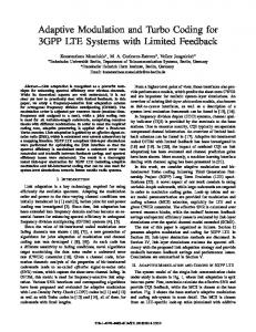
critical than in delay-sensitive interactive systems. More specifically, in their proposed scheme Berrou et al. [12, 13] used a parallel concatenation of two Recursive Systematic Convolutional (RSC) codes, accommodating the turbo interleaver between the two encoders. At the decoder an iterative structure using a modified version of the classic minimum BER MAP invented by Bahl et al. [11] was invoked by Berrou et al., in order to decode these parallel concatenated codes. Again, since 1993 a large amount of work has been carried out in the area, aiming for example to reduce the associated decoder complexity. Practical reduced-complexity decoders are for example the Max-Log-MAP algorithm proposed by Koch and Baier [50], as well as by Erfanian et al. [51], the Log-MAP algorithm suggested by Robertson, Villebrun and Hoeher [52], and the SOVA advocated by Hagenauer as well as Hoeher [53,54]. Le Goff, Glavieux and Berrou [55], Wachsmann and Huber [56] as well as Robertson and Worz [57] suggested the use of these codes in conjunction with bandwidth-efficient modulation schemes. Further advances in understanding the excellent performance of the codes are due, for example, to Benedetto and Montorsi [58, 59] and Perez, Seghers and Costello [60]. During the mid-1990s Hagenauer, Offer and Papke [61], as well as Pyndiah [62], extended the turbo concept to parallel concatenated block codes as well. Nickl et al. show in [63] that Shannon’s limit can be approached within 0.27 dB by employing a simple turbo Hamming code. In [64] Acikel and Ryan proposed an efficient procedure for designing the puncturing patterns for high-rate turbo convolutional codes. Jung and Nasshan [65, 66] characterised the achievable turbo-coded performance under the constraints of short transmission frame lengths, which is characteristic of interactive speech systems. In collaboration with Blanz they also applied turbo codes to a CDMA system using joint detection and antenna diversity [67]. Barbulescu and Pietrobon addressed the issues of interleaver design [68]. The tutorial paper by Sklar [69] is also highly recommended as background reading. Driven by the urge to support high data rates for a wide range of bearer services, Tarokh, Seshadri and Calderbank [70] proposed space-time trellis codes in 1998. By jointly designing the FEC, modulation, transmit diversity and optional receive diversity scheme, they increased the throughput of band-limited wireless channels. A few months later, Alamouti [71] invented a low-complexity space-time block code, which offers significantly lower complexity at the cost of a slight performance degradation. Alamouti’s invention motivated Tarokh et al. [72, 73] to generalise Alamouti’s scheme to an arbitrary number of transmitter antennas. Then, Tarokh et al., Bauch et al. [74, 75], Agrawal et al. [76], Li et al. [77, 78] and Naguib et al. [79] extended the research of space-time codes from considering narrowband channels to dispersive channels [70, 71, 73, 79, 80]. In Figure 1.1, we show the evolution of channel coding research over the past 50 years since Shannon’s legendary contribution [1]. These milestones have been incorporated also in the range of monographs and textbooks summarised in Figure 1.2. At the time of writing, the Shannon limit has been approached within 0.27 dB [63] over Gaussian channels. Also at the time of writing the challenge is to contrive FEC schemes which are capable of achieving a performance near the capacity of wireless channels.

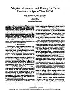
1.2 Motivation of the Book The design of an attractive channel coding and modulation scheme depends on a range of contradictory factors, which are portrayed in Figure 1.3. The message of this illustration is multi-fold. For example, given a certain transmission channel, it is always feasible to design a coding and modulation (‘codulation’) system, which can further reduce the BER achieved. This typically implies, however, further investments and/or penalties in terms of the required increased imple-

4


Convolutional Codes

Block Codes

Shannon limit [1] (1948) Hamming codes [3]

1950

Elias, Convolutional codes [3]

BCH codes [14–16] Reed-Solomon codes [30] PGZ algorithm [29]

1960

Berlekamp-Massey algorithm [31–34] RRNS codes [41, 42]

Viterbi algorithm [8] 1970

Chase algorithm [28] Bahl, MAP algorithm [11]

Wolf, trellis block codes [18] 1980

Ungerboeck, TCM [46, 47] 1990

Berrou, turbo codes [12, 13]

Pyndiah, SISO Chase algorithm [62, 81] Hagenauer, turbo BCH code [61] Nickl, turbo Hamming code [63] Alamouti, space-time block code [71]

Hagenauer, SOVA [53, 54] Koch, Max-Log-MAP algorithm [50, 51]

Robertson, Log-MAP algorithm [52]

2000

Robertson, TTCM [57] Tarokh, space-time trellis code [70] Acikel, punctured turbo code [64]

Figure 1.1: A brief history of channel coding.

1.3. ORGANISATION OF THE BOOK

5

mentational complexity and coding/interleaving delay as well as reduced effective throughput. Different solutions accrue when optimising different codec features. For example, in many applications the most important codec parameter is the achievable coding gain, which quantifies the amount of bit-energy reduction attained by a codec at a certain target BER. Naturally, transmitted power reduction is extremely important in battery-powered devices. This transmitted power reduction is only achievable at the cost of an increased implementational complexity, which itself typically increases the power consumption and hence erodes some of the power gain. Viewing this system optimisation problem from a different perspective, it is feasible to transmit at a higher bit rate in a given fixed bandwidth by increasing the number of bits per modulated symbol. However, when aiming for a given target BER, the channel coding rate has to be reduced, in order to increase the transmission integrity. Naturally, this reduces the effective throughput of the system and results in an overall increased system complexity. When the channel’s characteristic and the associated bit error statistics change, different solutions may become more attractive. This is because Gaussian channels, narrowband and wideband Rayleigh fading or various Nakagami fading channels inflict different impairments. These design trade-offs constitute the subject of this monograph.

Our intention with the book is multi-fold: 1) First, we would like to pay tribute to all researchers, colleagues and valued friends who contributed to the field. Hence this book is dedicated to them, since without their quest for better coding solutions to communications problems this monograph could not have been conceived. They are too numerous to name here, hence they appear in the author index of the book. 2) The invention of turbo coding not only assisted in attaining a performance approaching the Shannonian limits of channel coding for transmissions over Gaussian channels, but also revitalised channel coding research. In other words, turbo coding opened a new chapter in the design of iterative detection-assisted communications systems, such as turbo trellis coding schemes, turbo channel equalisers, etc. Similarly dramatic advances have been attained with the advent of space-time coding, when communicating over dispersive, fading wireless channels. Recent trends indicate that better overall system performance may be attained by jointly optimising a number of system components, such as channel coding, channel equalisation, transmit and received diversity and the modulation scheme, than in case of individually optimising the system components. This is the main objective of this monograph. 3) Since at the time of writing no joint treatment of the subjects covered by this book exists, it is timely to compile the most recent advances in the field. Hence it is our hope that the conception of this monograph on the topic will present an adequate portrayal of the last decade of research and spur this innovation process by stimulating further research in the coding and communications community.

1.3 Organisation of the Book Below, we present the outline and rationale of the book:

6


Shannon limit [1] (1948) 1950

1960

1970

Reed & Solomon, Polynomial codes over certain finite fields [30] Peterson, Error correcting codes [84] Wozencraft & Reiffen, Sequential decoding [5] Shannon, Mathematical theory of communication [91] Massey, Threshold decoding [7] Szabo & Tanaka, Residue arithmetic & its appl. to computer technology [41] Berlekamp, Algebraic coding theory [32] Kasami, Combinational mathematics and its applications [83] Peterson & Weldon, Error correcting codes [82] Blake, Algebraic coding theory: history and development [87]

Macwilliams & Sloane, The theory of error correcting codes [85] 1980

1990

2000

Clark & Cain, Error correction coding for digital communications [88] Pless, Introduction to the theory of error-correcting codes [89] Blahut, Theory and practice of error control codes [90] Lidl & Niederreiter, Finite fields [95] Lin & Costello, Error control coding: fundamentals and applications [96] Michelson & Levesque, Error control techniques for digital communication [97] Sklar, Digital communications fundamentals and applications [86] Sweeney, Error Control Coding: An Introduction [103] Hoffman et al., Coding theory [98] Huber, Trelliscodierung [99] Anderson & Mohan, Source and channel coding - an algorithmic approach [100] Wicker, Error control systems for digital communication and storage [101] Proakis, Digital communications [102] Honary & Markarian, Trellis decoding of block codes [19] S. Lin et al., Trellises & trellis-based decoding alg. for linear block codes [20] Schlegel, Trellis coding [48] Heegard & Wicker, Turbo coding [92] Bossert, Channel coding for telecommunications [93] Vucetic & Yuan, Turbo codes principles and applications [94] Hanzo, Liew & Yeap, Turbo coding, turbo equalisation & space-time coding, 2002 Figure 1.2: Milestones in channel coding.


7

Implementational complexity Coding/interleaving delay

Channel characteristics System bandwidth

Coding/ Modulation scheme

Effective throughput

Bit error rate Coding gain

Coding rate Figure 1.3: Factors affecting the design of channel coding and modulation scheme.

• Chapter 2: For the sake of completeness and wider reader appeal virtually no prior knowledge is assumed in the field of channel coding. Hence in Chapter 2 we commence our discourse by introducing the family of convolutional codes and the hard- as well as softdecision Viterbi algorithm in simple conceptual terms with the aid of worked examples. • Chapter 3: This chapter provides a rudimentary introduction to the most prominent classes of block codes, namely to Reed–Solomon (RS) and Bose–Chaudhuri– Hocquenghem (BCH) codes. A range of algebraic decoding techiques are also reviewed and worked examples are included. • Chapter 4: Based on the simple Viterbi decoding concepts introduced in Chapter 2, in this chapter an overview of the family of conventional binary BCH codes is given, with special emphasis on their trellis decoding. In parallel to our elaborations in Chapter 2 on the context of convolutional codes, the Viterbi decoding of binary BCH codes is detailed with the aid of worked examples. These discussions are followed by the simulation-based performance characterisation of various BCH codes employing both hard-decision and soft-decision decoding methods. The classic Chase algorithm is introduced and its performance is investigated. • Chapter 5: This chapter introduces the concept of turbo convolutional codes and gives a detailed discourse on the Maximum A-Posteriori (MAP) algorithm and its computationally less demanding counterparts, namely the Log-MAP and Max-Log-MAP algorithms. The Soft-Output Viterbi Algorithm (SOVA) is also highlighted and its concept is augmented with the aid of a detailed worked example. Then the effects of the various turbo codec parameters are investigated, namely that of the number of iterations, the puncturing patterns used, the component decoders, the influence of the interlever depth, which is related to the codeword length, etc. The various codecs’ performance is studied also when communicating over Rayleigh fading channels. • Chapter 6: While in Chapter 5 we invoked iterative turbo decoders, in this chapter a super-trellis is constructed from the two constituent convolutional codes’ trellises and the maximum likelihood codeword is output in a single, but implementationally coplex decoding step, without iterations. The advantage of the associated super-trellis is that it allows us to explore the trellis describing the construction of turbo codes and also to relate turbo codes to high-constraint-length convolutional codes of the same decoding complexity.

8


• Chapter 7: The concept of turbo codes using BCH codes as component codes is introduced. A detailed derivation of the MAP algorithm is given, building on the concepts introduced in Chapter 5 in the context of convolutional turbo codes, but this time cast in the framework of turbo BCH codes. Then, the MAP algorithm is modified in order to highlight the concept of the Max-Log-MAP and Log-MAP algorithms, again, with reference to binary turbo BCH codes. Furthermore, the SOVA-based binary BCH decoding algorithm is introduced. Then a simple turbo decoding example is given, highlighting how iterative decoding assists in correcting multiple errors. We also describe a novel MAP algorithm for decoding extended BCH codes. Finally, we show the effects of the various coding parameters on the performance of turbo BCH codes. • Chapter 8: The concept of Residue Number Systems (RNS) is introduced and extended to Redundant Residue Number Systems (RRNS), introducing the family of RRNS codes. Some coding-theoretic aspects of RRNS codes is investigated, demonstrating that RRNS codes exhibit similar distance properties to RS codes. A procedure for multiple-error correction is then given. Different bit-to-symbol mapping methods are highlighted, yielding non-systematic and systematic RRNS codes. A novel bit-to-symbol mapping method is introduced, which results in efficient systematic RRNS codes. The classic Chase algorithm is then modified in order to create a Soft-Input Soft-Output (SISO) RRNS decoder. This enables us to implement the iterative decoding of turbo RRNS codes. Finally, simulation results are given for various RRNS codes, employing hard-decision and soft-decision decoding methods. The performance of the RRNS codes is compared to that of RS codes and the performance of turbo RRNS codes is studied. • Chapter 9: Our previous discussions on various channel coding schemes evolves to the family of joint coding and modulation-based arrangements, which are often referred to as coded modulation schemes. Specifically, Trellis-Coded Modulation (TCM), Turbo TrellisCoded Modulation (TTCM), Bit-Interleaved Coded Modulation (BICM) as well as iterative joint decoding and demodulation-assisted BICM (BICM-ID) will be studied and compared under various narrowband and wideband propagation conditions. • Chapter 10: Space-time block codes are introduced. The derivation of the MAP decoding of space-time block codes is then given. A system is proposed by concatenating space-time block codes and various channel codes. The complexity and memory requirements of various channel decoders are derived, enabling us to compare the performance of the proposed channel codes by considering their decoder complexity. Our simulation results related to space-time block codes using no channel coding are presented first. Then, we investigate the effect of mapping data and parity bits from binary channel codes to non-binary modulation schemes. Finally, we compare our simulation results for various channel codes concatenated with a simple space-time block code. Our performance comparisons are conducted by also considering the complexity of the associated channel decoder. • Chapter 11: The encoding process of space-time trellis codes is highlighted. This is followed by employing an Orthogonal Frequency Division Multiplexing (OFDM) modem in conjunction with space-time codes over wideband channels. Turbo codes and RS codes are concatenated with space-time codes in order to improve their performance. Then, the performance of the advocated space-time block code and space-time trellis codes is compared. Their complexity is also considered in comparing both schemes. The effect of delay spread and maximum Doppler frequency on the performance of the space-time codes is investigated. A Signal to Interference Ratio (SIR) related term is defined in the context


9

of dispersive channels for the advocated space-time block code, and we will show how the SIR affects the performance of the system. In our last section, we propose space-timecoded Adaptive OFDM (AOFDM). We then show by employing multiple antennas that with the advent of space-time coding, the wideband fading channels have been converted to AWGN-like channels. • Chapter 12: The discussions of Chapters 10 and 11 were centred around the topic of employing multiple-transmitter, multiple-receiver (MIMO) based transmit and receivediversity assisted space-time coding schemes. These arrangements have the potential of significantly mitigating the hostile fading wireless channel’s near-instantaneous channel quality fluctuations. Hence these space-time codecs can be advantageously combined with powerful channel codecs originally designed for Gaussian channels. As a lower-complexity design alternative, this chapter introduces the concept of nearinstantaneously Adaptive Quadrature Amplitude Modulation (AQAM), combined with near-instantaneously adaptive turbo channel coding. These adaptive schemes are capable of mitigating the wireless channel’s quality fluctuations by near-instantaneously adapting both the modulation mode used as well as the coding rate of the channel codec invoked. The design and performance study of these novel schemes constitutes the topic of Chapter 12. • Chapter 13: This chapter focuses on the portrayal of partial-response modulation schemes, which exhibit impressive performance gains in the context of joint iterative, joint channel equalisation and channel decoding. This joint iterative receiver principle is termed turbo equalisation. An overview of Soft-In/Soft-Out (SISO) algorithms, namely that of the MAP algorithm and Log-MAP algorithm, is presented in the context of GMSK channel equalisation, since these algorithms are used in the investigated joint channel equaliser and turbo decoder scheme. • Chapter 14: Based on the introductory concepts of Chapter 13, in this chapter the detailed principles of iterative joint channel equalisation and channel decoding techniques known as turbo equalisation are introduced. This technique is invoked in order to overcome the unintentional Inter-Symbol Interference (ISI) and Controlled Inter-Symbol Interference (CISI) introduced by the channel and the modulator, respectively. Modifications of the SISO algorithms employed in the equaliser and decoder are also portrayed, in order to generate information related not only to the source bits but also to the parity bits of the codewords. The performance of coded systems employing turbo equalisation is analysed. Three classes of encoders are utilised, namely convolutional codes, convolutional-codingbased turbo codes and BCH-coding-based turbo codes. • Chapter 15: Theoretical models are devised for the coded schemes in order to derive the maximum likelihood bound of the system. These models are based on the Serial Concatenated Convolutional Code (SCCC) analysis presented in reference [104]. Essentially, this analysis can be employed since the modulator could be represented accurately as a rate R = 1 convolutional encoder. Apart from convolutional-coded systems, turbo-coded schemes are also considered. Therefore the theoretical concept of Parallel Concatenated Convolutional Codes (PCCC) [59] is utilised in conjunction with the SCCC principles in order to determine the Maximum Likelihood (ML) bound of the turbo-coded systems, which are modelled as hybrid codes consisting of a parallel concatenated convolutional code, serially linked with another convolutional code. An abstract interleaver from reference [59] — termed the uniform interleaver — is also utilised, in order to reduce the

10


complexity associated with determining all the possible interleaver permutations. • Chapter 16: A comparative study of coded BPSK systems, employing high-rate channel encoders, is presented. The objective of this study is to investigate the performance of turbo equalisers in systems employing different classes of codes for high code rates of R = 34 and R = 56 , since known turbo equalisation results have only been presented for turbo equalisers using convolutional codes and convolutional-based turbo codes for code rates of R = 13 and R = 21 [105, 106]. Specifically, convolutional codes, convolutionalcoding-based turbo codes, and Bose–Chaudhuri–Hocquengham (BCH)-coding-based [14, 15] turbo codes are employed in this study. • Chapter 17: A novel reduced-complexity trellis-based equaliser is presented. In each turbo equalisation iteration the decoder generates information which reflects the reliability of the source and parity bits of the codeword. With successive iteration, the reliability of this information improves. This decoder information is exploited in order to decompose the received signal such that each quadrature component consists of the in-phase or quadrature-phase component signals. Therefore, the equaliser only has to consider the possible in-phase or quadrature-phase components, which is a smaller set of signals than all of their possible combinations. • Chapter 18: For transmissions over wideband fading channels and fast fading channels, space-time trellis coding (STTC) is a more appropriate diversity technique than space-time block coding. STTC [70] relies on the joint design of channel coding, modulation, transmit diversity and the optional receiver diversity schemes. The decoding operation is performed by using a maximum likelihood detector. This is an effective scheme, since it combines the benefits of Forward Error Correction (FEC) coding and transmit diversity, in order to obtain performance gains. However, the cost of this is the additional computational complexity, which increases as a function of bandwidth efficiency (bits/s/Hz) and the required diversity order. In this chapter STTC is investigated for transmission over wideband fading channels. • Chapter 19: This chapter provides a brief summary of the book. It is our hope that this book portrays the range of contradictory system design trade-offs associated with the conception of channel coding arrangements in an unbiased fashion and that readers will be able to glean information from it in order to solve their own particular channel coding and communications problem. Most of all, however, we hope that they will find it an enjoyable and informative read, providing them with intellectual stimulation.

Lajos Hanzo, Tong Hooi Liew and Bee Leong Yeap Department of Electronics and Computer Science University of Southampton

Part I

Convolutional and Block Coding

Chapter

2

Convolutional Channel Coding 2.1 Brief Channel Coding History In this chapter a rudimentary introduction to convolutional coding is offered to those readers who are not familiar with the associated concepts. Readers who are familiar with the basic concepts of convolutional coding may proceed to the chapter of their immediate interest. The history of channel coding or Forward Error Correction (FEC) coding dates back to Shannon’s pioneering work in which he predicted that arbitrarily reliable communications are achievable by redundant FEC coding, although he refrained from proposing explicit schemes for practical implementations. Historically, one of the first practical codes was the single error correcting Hamming code [2], which was a block code proposed in 1950. Convolutional FEC codes date back to 1955 [3], which were discovered by Elias, whereas Wozencraft and Reiffen [4,5], as well as Fano [6] and Massey [7], proposed various algorithms for their decoding. A major milestone in the history of convolutional error correction coding was the invention of a maximum likelihood sequence estimation algorithm by Viterbi [8] in 1967. A classic interpretation of the Viterbi Algorithm (VA) can be found, for example, in Forney’s often-quoted paper [9], and one of the first applications was proposed by Heller and Jacobs [107]. We note, however, that the VA does not result in minimum Bit Error Rate (BER). The minimum BER decoding algorithm was proposed in 1974 by Bahl et al. [11], which was termed the Maximum A-Posteriori (MAP) algorithm. Although the MAP algorithm slightly outperforms the VA in BER terms, because of its significantly higher complexity it was rarely used, until turbo codes were contrived [12]. During the early 1970s, FEC codes were incorporated in various deep-space and satellite communications systems, and in the 1980s they also became common in virtually all cellular mobile radio systems. A further historic breakthrough was the invention of the turbo codes by Berrou, Glavieux, and Thitimajshima [12] in 1993, which facilitates the operation of communications systems near the Shannonian limits. Focusing our attention on block codes, the single error correcting Hamming block code was too weak, however, for practical applications. An important practical milestone was the discovery of the family of multiple error correcting Bose–Chaudhuri–Hocquenghem (BCH) binary block codes [14] in 1959 and in 1960 [15, 16]. In 1960, Peterson [17] recognised that these codes exhibit a cyclic structure, implying that all cyclically shifted versions of a legitimate codeword are also legitimate codewords. Furthermore, in 1961 Gorenstein and Zierler [29] extended the 13

14

CHAPTER 2. CONVOLUTIONAL CHANNEL CODING

binary coding theory to treat non-binary codes as well, where code symbols were constituted by a number of bits, and this led to the birth of burst-error correcting codes. They also contrived a combination of algorithms, which are referred to as the Peterson–Gorenstein–Zierler (PGZ) algorithm. We will elaborate on this algorithm later in this chapter. In 1960 a prominent nonbinary subset of BCH codes were discovered by Reed and Solomon [30]; they were named Reed– Solomon (RS) codes after their inventors. These codes exhibit certain optimality properties, and they will also be treated in more depth in this chapter. We will show that the PGZ decoder can also be invoked for decoding non-binary RS codes. A range of powerful decoding algorithms for RS codes was found by Berlekamp [31,32] and Massey [33, 34], which also constitutes the subject of this chapter. In recent years, these codes have found practical applications, for example, in Compact Disc (CD) players, in deep-space scenarios [38], and in the family of Digital Video Broadcasting (DVB) schemes, which were standardised by the European Telecommunications Standardization Institute (ETSI). We now consider the conceptually less complex class of convolutional codes, which will be followed by our discussions on block coding.

2.2 Convolutional Encoding Both block codes and Convolutional Codes (CCs) can be classified as systematic or nonsystematic codes, where the terminology suggests that in systematic codes the original information bits or symbols constitute part of the encoded codeword and hence they can be recognised explicitly at the output of the encoder. Their encoders can typically be implemented by the help of linear shift-register circuitries, an example of which can be seen in Figure 2.1. The figure will be explored in more depth after introducing some of the basic convolutional coding parameters. Specifically, in general a k-bit information symbol is entered into the encoder, constituted by K shift-register stages. In our example of Figure 2.1, the corresponding two shift-register stages are s1 and s2 . In general, the number of shift-register stages K is referred to as the constraint length of the code. An alternative terminology is to refer to this code as a memory three code, implying that the memory of the CC is given by K + 1. The current shift-register state s1 , s2 plus the incoming bit bi determine the next state of this state machine. The number of output bits is typically denoted by n, while the coding rate by R = k/n, implying that R ≤ 1. In order to fully specify the code, we also have to stipulate the generator polynomial, which describes the topology of the modulo-2 gates generating the output bits of the convolutional encoder. For generating n bits, n generator polynomials are necessary. In general, a CC is denoted as a CC(n, k, K) scheme, and given the n generator polynomials, the code is fully specified. Once a specific bit enters the encoder’s shift register in Figure 2.1, it has to traverse through the register, and hence the register’s sequence of state transitions is not arbitrary. Furthermore, the modulo-2 gates impose additional constraints concerning the output bit-stream. Because of these constraints, the legitimate transmitted sequences are restricted to certain bit patterns, and if there are transmission errors, the decoder will conclude that such an encoded sequence could not have been generated by the encoder and that it must be due to channel errors. In this case, the decoder will attempt to choose the most resemblent legitimately encoded sequence and output the corresponding bit-stream as the decoded string. These processes will be elaborated on in more detail later in the chapter. The n generator polynomials g1 , g2 , . . . , gn are described by the specific connections to the register stages. Upon clocking the shift register, a new information bit is inserted in the register, while the bits constituting the states of this state machine move to the next register stage and the last bit is shifted out of the register. The generator polynomials are constituted by a binary

2.2. CONVOLUTIONAL ENCODING

15

Output 6

J:10 9 8 7 6 5 4 3 2 1 ...0 0 1 1 0 1 1 0 0 0

-

s1

bi -

s2

-

bi

bp

-

? q

J 1 2 3 4 5 6 7 8 9 10

Input bi 0 0 0 1 1 0 1 1 0 0

+

=

s1 0 0 0 0 1 1 0 1 1 0

s2 0 0 0 0 0 1 1 0 1 1

Output bp bi 0 0 0 0 0 0 1 1 0 1 0 0 0 1 0 1 0 0 0 1

Figure 2.1: Systematic half-rate, constraint-length two convolutional encoder CC(2, 1, 2).

pattern, indicating the presence or absence of a specific link from a shift register stage by a binary one or zero, respectively. For example, in Figure 2.1 we observe that the generator polynomials are constituted by: g1 = [1 0 0] and g2 = [1 1 1] ,

(2.1)

or, in an equivalent polynomial representation, as: g1 (z) = 1 + 0 · z 1 + 0 · z 2 and g2 (z) = 1 + z + z 2 .

(2.2)

We note that in a non-systematic CC, g1 would also have more than one non-zero term. It is intuitively expected that the more constraints are imposed by the encoder, the more powerful the code becomes, facilitating the correction of a higher number of bits, which renders nonsystematic CCs typically more powerful than their systematic counterparts. Again, in a simple approach, we will demonstrate the encoding and decoding principles in the context of the systematic code specified as (k = 1), half-rate (R = k/n = 1/2), CC(2, 1, 2), with a memory of three binary stages (K = 2). These concepts can then be extended to arbitrary codecs. At the commencement of the encoding, the shift register is typically cleared by setting it to the all-zero state, before the information bits are input to it. Figure 2.1 demonstrates the encoder’s operation for the duration of the first ten clock cycles, tabulating the input bits, the

16


bi bp = 00

*

s1 s2 = 00 bi bp = 11

00

’0’’1’-

bi bp = 01 s1 s2 = 01

*

bi bp = 10

01

bi bp = 01 s1 s2 = 10

R6 j

bi bp = 00

10

bi bp = 10 q

s1 s2 = 11

-

11

bi bp = 11

Figure 2.2: State transition diagram of the CC(2, 1, 2) systematic code, where broken lines indicate transitions due to an input one, while continuous lines correspond to input zeros.

shift-register states s1 , s2 , and the corresponding output bits. At this stage, the uninitiated reader is requested to follow the operations summarised in the figure before proceeding to the next stage of operations.

2.3 State and Trellis Transitions An often-used technique for characterising the operations of a state machine, such as our convolutional encoder, is to refer to the state transition diagram of Figure 2.2. Given that there are two bits in the shift register at any moment, there are four possible states in the state machine and the state transitions are governed by the incoming bit bi . A state transition due to a logical zero is indicated by a continuous line in the figure, while a transition activated by a logical one is represented by a broken line. The inherent constraints imposed by the encoder manifest themselves here in that from any state there are only two legitimate state transitions, depending on the binary input bit. Similarly, in each state there are two merging paths. It is readily seen from the encoder circuit of Figure 2.1 that, for example, from state (s1 , s2 )=(1,1) a logical one input results in a transition to (1,1), while an input zero leads to state (0,1). The remaining transitions can also be readily checked by the reader. A further feature of this figure is that the associated encoded output bits are also plotted in the boxes associated with each of the transitions. Hence,

2.3. STATE AND TRELLIS TRANSITIONS

J=1 00 00

J=2 J=3 J=4 00 00 -

17

J=5

J=6

J=7

J=9 J=10 J=11

J=8

01

11

01

10

11

00 W

00

10 U

10

10

U

U

Figure 2.3: Trellis-diagram of the CC(2, 1, 2) systematic code, where broken lines indicate transitions due to a binary one, while continuous lines correspond to input zeros.

this diagram fully describes the operations of the encoder. Another simple way of characterising the encoder is to portray its trellis diagram, which is depicted in Figure 2.3. At the left of the figure, the four legitimate encoder states are portrayed. Commencing operations from the all-zero register state (0,0) allows us to mirror the encoder’s actions seen in Figures 2.1 and 2.2 also in the trellis diagram, using the same input bit-stream. As before, the state transitions are governed by the incoming bits bi and a state transition due to a logical zero is indicated by a continuous line, while a transition activated by a logical one is represented by a broken line. Again, the inherent constraints imposed by the encoder manifest themselves here in that from any state there are only two legitimate state transitions, depending on the binary input bit, and in each state there are two merging paths. Given our specific input bit-stream, it is readily seen from the encoder circuit of Figure 2.1 and the state transition diagram of Figure 2.2 that, for example, from state (s1 , s2 )=(0,0) a logical zero input bit results in a transition to (0,0), while an input one leads to state (1,0). The remaining transitions shown in the figure are associated with our specific input bit-stream, which can be readily explored by the reader. As before, the associated output bits are indicated in the boxes along each of the transitions. Hence, the trellis diagram gives a similarly unambiguous description of the encoder’s operations to the state diagram of Figure 2.2. Armed with the above description of CCs, we are now ready to give an informal description of the maximum likelihood Viterbi algorithm in the next section.

18


J=1

2

3

4

5

6

7

8

9

survivor path

00

1 00

1 00

2

s1s2=00

2

4 11

11

2

2

4 01

4

01

2

01

discarded paths

5

2

s1s2=01 01

s1s2=10

01

3

3

00

00

3

1 10

10 3

s1s2=11

3

2

4

11

11

RANDOM DECISION Received

:

10

00

10

00

00

00

00

00

Decoded

:

0

0

0

0

0

0

0

0

Figure 2.4: Trellis-diagram-based Viterbi decoding of the CC(2, 1, 2) systematic code, where broken lines indicate transitions due to an input one, while continuous lines correspond to input zeros — error-free hard-decision decoding of two isolated bit errors.

2.4 The Viterbi Algorithm 2.4.1

Error-free Hard-decision Viterbi Decoding

Given the received bit-stream, the decoder has to arrive at the best possible estimate of the original uncoded information sequence. Hence, the previously mentioned constraints imposed by the encoder on the legitimate bit sequences have to be exploited in order to eradicate illegitimate sequences and thereby remove the transmission errors. For the sake of computational simplicity, let us assume that the all-zero bit-stream has been transmitted and the received sequence of Figure 2.4 has been detected by the demodulator, which has been passed to the FEC decoder. We note

2.4. THE VITERBI ALGORITHM

19

here that if the demodulator carries out a binary decision concerning the received bit, this operation is referred to as hard-decision demodulation. By contrast, if the demodulator refrains from making a binary decision and instead it outputs a more finely graded multilevel confidence measure concerning the probability of a binary one and a binary zero, then it is said to invoke soft-decision demodulation. For the time being we will consider only hard-decision demodulation. The decoder now has to compare the received bits with all the legitimate sequences of the trellis diagram of Figure 2.4 and quantify the probability of each of the associated paths, which ultimately assigns a probability-related quantity to specific decoded sequences, as we will show below. Referring to Figure 2.4 and beginning the decoding operations from the all-zero state, we compute the Hamming distance of the received two-bit symbol with respect to both of the legitimate encoded sequences of the trellis diagram for the first trellis section (i.e. for the first trellis transition), noting that the Hamming distance is given by the number of different bit positions between two binary sequences. For example, for the first two-bit received symbol 10, the associated Hamming distances are 1 with respect to both the 00 and the 11 encoded sequences. Thus, at this stage the decoder is unable to express any preference as to whether 00 or 11 was the more likely transmitted symbol. We also note these Hamming distances in the trellis diagram of Figure 2.4, indicated at the top of the nodes corresponding to the new encoder states we arrived at, as a consequence of the state transitions due to a logical one and zero, respectively. These Hamming distances are known in the context of Viterbi decoding as the branch metric. The power of the Viterbi decoding algorithm accrues from the fact that it carries out a maximum likelihood sequence estimation, as opposed to arriving at symbol-by-symbol decisions, and thereby exploits the constraints imposed by the encoder on the legitimate encoded sequences. Hence, the branch metrics will be accumulated over a number of consecutive trellis stages before a decision as to the most likely encoder path and information sequence can be released. Proceeding to the next received two-bit symbol, namely 00, the operations of the decoder are identical; that is, the Hamming distance between the encoded symbols of all four legitimate paths and the received symbol is computed. These distances yield the new branch metrics associated with the second trellis stage. By now the encoded symbols of two original input bits have been received, and this is why there are now four possible trellis states in which the decoder may reside. The branch metrics computed for these four legitimate transitions from top to bottom are 0, 2, 1 and 1, respectively. These are now added to the previous branch metrics of 1 in order to generate the path metrics of 1, 2, 3 and 2, respectively, quantifying the probability of each legitimate trellis path in terms of the accumulated Hamming distance. A low Hamming distance indicates a high similarity between the received sequence and the encoded sequence concerned, which is characteristic of the most likely encoded sequence, since the probability of a high number of errors is exponentially decreasing with the number of errors. Returning to Figure 2.4 again, the corresponding accumulated Hamming distances or branch metrics from top to bottom are 1, 2, 3 and 2, respectively. At this stage, we can observe that the top branch has the lowest branch metric and hence it is the most likely encountered encoder path. The reader knows this, but the decoder can only quantify the probability of the corresponding paths and thus it cannot be sure of the validity of its decision. The other three encoder paths and their associated information bits also have a finite probability. Continuing the legitimate paths of Figure 2.4 further, at trellis stage three the received sequence of 10 is compared to the four legitimate two-bit encoded symbols and the associated path metrics now become dependent on the actual path followed, since at this stage there are merging paths. For example, at the top node we witness the merger of the 00, 00, 00 path with the 11, 01, 01 path, where the associated original information bits were 0,0,0 and 1,0,0, respectively. On

20


the basis of the associated path metrics, the decoder may ‘suspect’ that the former one was the original information sequence, but it still refrains from carrying out a decision. Considering the two merging paths, future input bits would affect both of these in an identical fashion, resulting in an indistinguishable future set of transitions. Their path metrics will therefore also evolve identically, suggesting that it is pointless to keep track of both of the merging paths, since the one with the lower metric will always remain the more likely encoder path. This is reflected in Figure 2.4 by referring to the path exhibiting the lower metric as the survivor path, while the higher metric merging path will be discarded. We also note that at the bottom node of trellis stage three we ended up with two identical path metrics, namely 3, and in this case a random decision must be made as to which one becomes the survivor. This event is indicated in Figure 2.4 by the arrow. In this particular example, this decision does not affect the final outcome of the decoder’s decision, since the top path appears to be the lowest metric path. Nonetheless, in some situations such random decisions will influence the decoded bit sequence and may indeed determine whether decoding errors are encountered. It is plausible that the confidence in the decoder’s decision is increased, as the accumulation of the branch metrics continues. Indeed, one may argue that the ‘best’ decision can be taken upon receiving the complete information sequence. However, deferring decisions for so long may not be acceptable in latency terms, in particular in delay-sensitive interactive speech or video communications. Nor is it necessary in practical terms, since experience shows that the decoder’s bit error rate is virtually unaffected by curtailing the decision interval to about five times the encoder’s memory, which was three in our example. In our example, the received bit sequence does not contain any more transmission errors, and so it is plausible that the winning path remains the one at the top of Figure 2.4 and the associated branch metric of 2 reflects the actual number of transmission errors. We are now ready to release the error-free decoded sequence, namely the all-zero sequence, as seen explicitly in terms of the corresponding binary bits at the bottom of Figure 2.4. The corresponding winning path was drawn in bold in the figure.

2.4.2

Erroneous Hard-decision Viterbi Decoding

Following the above double-error correction scenario, below we consider another instructive example where the number of transmission errors remains two and even their separation is increased. Yet the decoder may become unable to correct the errors, depending on the outcome of a random decision. This is demonstrated in Figure 2.5 at stage four of the top path. Observe furthermore that the corresponding received bits and path metrics of Figure 2.4 are also indicated in Figure 2.5, but they are crossed out and superseded by the appropriately updated values according to the current received pattern. Depending on the actual choice of the survivor path at stage four, the first decoded bit may become a logical one, as indicated at the bottom of Figure 2.5. The accumulated Hamming distance becomes 2, regardless of the random choice of the survivor path, which indicates that in the case of decoding errors the path metric is not a reliable measure of the actual number of errors encountered. This will become even more evident in our next example. Let us now consider a scenario in which there are more than two transmission errors in the received sequence, as seen in Figure 2.6. Furthermore, the bit errors are more concentrated, forming a burst of errors, rather than remaining isolated error events. In this example, we show that the decoder becomes ‘overloaded’ by the plethora of errors, and hence it will opt for an erroneous trellis path, associated with the wrong decoded bits. Observe in Figure 2.4 that up to trellis stage three the lowest-metric path is the one at the


2

J=1

21

3

4

5

6

7

8

9

random decision

00

1 00

1 00

s1s2=00 11

11

01

2

s1s2=01

1

2

4 2 01

4 4

2

2

2

4 01

3 5

01

s1s2=10

2

01

3

3

00

00

3

10

10 5

s1s2=11

3

2

5

11

11

Received

:

10

00

01 10

00

00

00

00

00

Decoded

:

0 1

0 0

0 0

0 0

0 0

0 0

0 0

0 0

or

Figure 2.5: Trellis-diagram-based Viterbi decoding of the CC(2, 1, 2) systematic code, where broken lines indicate transitions due to an input one, while continuous lines correspond to input zeros — erroneous hard-decision decoding of two isolated bit errors.

22


J=1

J=2

J=3

b 1b2=00 b 1b2=00 s1 s2=00

0

0

11

J=4

J=6

J=8

J=9

J=10

J=11

1

1

1

1 0

11

01

3

01 0

0 01

s1 s2=10

J=7

00 0 4

01

s1 s2=01

J=5

00

2 10

10

0

0

10

10

00

0 s1 s2=11

3

0

Received Bits :

00

00

00

11

10

00

10

10

00

01

Decoded Bits :

0

0

0

1

1

0

1

1

0

0

Figure 2.6: Trellis-diagram-based Viterbi decoding of the CC(2, 1, 2) systematic code, where broken lines indicate transitions due to an input one, while continuous lines correspond to input zeros — erroneous hard-decision decoding of burst errors.

top, which is associated with the error-free all-zero sequence. However, the double error in the fourth symbol of Figure 2.6 results in a ‘dramatic’ turn of events, since the survivor path deviates from the error-free all-zero sequence. Because of the specific received sequence encountered, the path metric remains 0 up to trellis stage J = 11, the last stage, accumulating a total of zero Hamming distance, despite actually encountering a total of six transmission errors, resulting in four decoding errors at the bottom of Figure 2.6. Again, the winning path was drawn in bold in Figure 2.4. From this experience we can infer two observations. First, the high-error rate scenario encountered is less likely than the previously considered double-error case, but it has a finite probability and hence it may be encountered in practice. Second, since the decoder carries out a maximum likelihood decision, in such cases it will opt for the wrong decoded sequence, in which case the accumulated path metric will not correctly reflect the number of transmission errors encountered. We therefore conclude that, in contrast to block codes, CCs do not possess an ability to monitor the number of transmission errors encountered.


2.4.3

23

Error-free Soft-decision Viterbi Decoding

Having considered a number of hard-decision decoding scenarios, let us now demonstrate the added power of soft-decision decoding. Recall from our earlier discussions that if the demodulator refrains from making a binary decision and instead it outputs a finely graded soft-decision confidence measure related to the probability of a binary one and a binary zero, respectively, then it is said to invoke soft-decision demodulation. As an example, we may invoke an eightlevel soft-decision demodulator output. This provides a more accurate indication of whether the demodulator’s decision concerning a certain demodulated bit is a high- or low-reliability one. This clearly supplies the Viterbi decoder with substantially more information than the previous binary zero/one decisions. Hence, a higher error correction capability will be achieved, as we will demonstrate in Figure 2.7. Specifically, let us assume that on our eight-level confidence scale +4 indicates the highest possible confidence concerning the demodulator’s decision for a binary one and -4 the lowest possible confidence. In fact, if the demodulator outputs -4, the low confidence in a logical one implies a high confidence in a logical zero, and conversely, the demodulator output of +4 implies a very low probability of a binary zero. Bearing this eight-level confidence scale of [-4, -3, ... +3, +4] in mind, the previously erroneously decoded double-error scenario of Figure 2.5 can now be revisited in Figure 2.7, where we will demonstrate that the more powerful soft-decision decoding allows us to remove all transmission errors. Let us first consider the soft-decision metrics provided by the demodulator, which now replace the previously used hard-decision values at the bottom of Figure 2.5, appearing crossed out in Figure 2.7. For example, the first two values appear to be a high-confidence one and zero, respectively. The second two values are relatively high-confidence zeros, whereas the previously erroneously demodulated third symbol, namely 01, is now represented by the confidence values of -2,+1, indicating that these bits may well have been either one or zero. The rest of the soft-decision metrics appear to be of higher value, apart from the last-but-one. The computation of the branch metrics and path metrics now has to be slightly modified. Previously, we were accumulating only ‘penalties’ in terms of the Hamming distances encountered. By contrast, in soft-decision decoding we will have to accumulate both penalties and credits, since we now consider the possibility of all demodulated values being both a binary one and a zero and quantify their associated probabilities using the soft-decision (SD) metrics. Explicitly, in Figure 2.7 we replace the crossed-out hard-decision metrics by the corresponding soft-decision metrics. Considering trellis stage one and the 00 encoded symbol, the first SD metric of +3 does not tally well with the bit zero; rather, it indicates a strong probability of a one; hence, we accumulate a ‘penalty’ of -3. The second SD metric, however, indicates a strong probability of a zero, earning a credit of +3, which cancels the previous -3 penalty, yielding a SD branch metric of 0. Similar arguments are valid for the trellis branch from (0,0) to (1,0), which is associated with the encoded symbol 11, also yielding a SD branch metric of 0. During stage two, the received SD metrics of -2,-3 suggest a high probability of two zeros, earning an added credit of +5 along the branch (0,0) to (0,0). By contrast, these SD values do not tally well with the encoded symbol of 11 along the transition of (0,0) to (1,0), yielding a penalty of -5. During the third stage along the path from (0,0) to (0,0), we encounter a penalty of -1 and a credit of +2, bringing the total credits for the all-zero path to +6. At this stage of the hard-decision decoder of Figure 2.7, we encountered a random decision, which now will not be necessary, since the merging path has a lower credit of +2. Clearly, at trellis stage nine we have a total credit of +29, allowing the decoder to release the correct original all-zero information sequence.

24


J=1

2

3

0

+5

4

5

6

7

8

9

+18

2

+23

+25

+29

2

2

survivor path

00

1 00

+6

1 00

00

2

s1s2=00

+11

2 00

11

01

-1

-2

2

3

s1s2=01 01

0

s1s2=10

+2

01

+4

4

2 11

01

01

+3

3 +2

3 +5

00

00

-5

1

3

10

10 -8 -5

5 s1s2=11

+1

+3,-3

3

2

5

11 0

-2,-3

-2,+1

11

-3,-2

-3,-4

-2,-3

-1,-1

-2,-2

Received

:

10

00

01

00

00

00

00

00

Decoded

:

0

0

0

0

0

0

0

0

Figure 2.7: Trellis-diagram-based Viterbi decoding of the CC(2, 1, 2) systematic code, where broken lines indicate transitions due to an input one, while continuous lines correspond to input zeros — error-free soft-decision decoding of two isolated bit errors.

2.5. SUMMARY AND CONCLUSIONS

25

2.5 Summary and Conclusions This brief chapter commenced by providing a historical perspective on convolution coding. The convolutional encoder has been characterised with the aid of its state transition diagram and trellis diagram. Then the classic Viterbi algorithm has been introduced in the context of a simple decoding example, considering both hard- and soft-decision-based scenarios. In the next chapter, we focus our attention on the family of block codes, which have found numerous applications in both standard and proprietary wireless communications systems. A variety of video schemes characterised in this monograph have also opted for employing Bose–Chaudhuri–Hocquenghem codes.

Chapter

3

Block Coding 3.1 Introduction Having studied the basics of convolutional coding in the previous chapter, we now focus our attention on methods of combatting transmission errors with the aid of block codes. The codes discussed in this chapter have found favour in numerous standard communications systems and hence they are historically important. While a basic understanding of the construction of these codes is important for equipping the reader with the necessary background for studying turbo Bose–Chaudhuri–Hocquenghem codes, for example, the full appreciation of the associated socalled algebraic decoding techniques discussed in this this chapter is not necessary. After demodulating the received signal, transmission errors can be removed from the digital information if their number does not exceed the error correcting power of the error correction code used. The employment of Forward Error Correction (FEC) coding techniques becomes important for transmissions over hostile mobile radio channels, where the violent channel fading precipitates bursts of error. This is particularly true when using vulnerable multilevel modulation schemes, such as Quadrature Amplitude Modulation (QAM). This chapter addresses issues of Reed–Solomon (RS) and Bose–Chaudhuri–Hocquenghem (BCH) coding in order to provide a self-contained reference for readers who want to delve into the theory of FEC coding. The theory and practice of FEC coding has been well documented in classic references [32, 82, 84, 87–90, 96, 97]; hence for an in-depth treatment, the reader is referred to these sources. Both convolutional and block FEC codes have been successfully utilised in various communications systems [108, 109]. In this brief overview, to a certain extent we will follow the philosophy of these references, which are also recommended for a more detailed discourse on the subject. Since the applications described in this book often use the family of RS and BCH block codes, in this chapter we concentrate on their characterisation. We will draw the reader’s attention to any differences between them, as they arise during our discussions. Both RS and BCH codes are defined over the mathematical structure of finite fields; therefore we briefly consider their construction. For a more detailed discourse on finite fields, the reader is referred to Lidl’s work [95]. 27

28

CHAPTER 3. BLOCK CODING

+ 0 1 2 3 4 5 6

0 0 1 2 3 4 5 6

1 1 2 3 4 5 6 0

2 2 3 4 5 6 0 1

3 3 4 5 6 0 1 2

4 4 5 6 0 1 2 3

5 5 6 0 1 2 3 4

6 6 0 1 2 3 4 5

× 0 1 2 3 4 5 6

0 0 0 0 0 0 0 0

1 0 1 2 3 4 5 6

2 0 2 4 6 1 3 5

3 0 3 6 2 5 1 4

4 0 4 1 5 2 6 3

5 0 5 3 1 6 4 2

6 0 6 5 4 3 2 1

Table 3.1: M odulo − 7 addition and multiplication tables for the prime field. GF (7)

3.2 Finite Fields 3.2.1

Definitions

Loosely speaking, an algebraic field is any arithmetic structure in which addition, subtraction, multiplication and division are defined and the associative, distributive and commutative laws apply. In conventional algebraic fields, like the rational, real or complex field, these operations are trivial, but in other fields they are somewhat different, such as modulo or modulo polynomial operations. A more formal field definition can be formulated as follows [90]. An algebraic field is a set of elements that has addition and multiplication defined over it, such that the set is closed under both addition and multiplication; that is, the results of these operations are also elements in the same set. Furthermore, both addition and multiplication are associative and commutative. There is a zero element, such that a + 0 = a, and an additive inverse element, such that a + (−a) = 0. Subtraction is defined as a − b = a + (−b). There is a one element, such that 1 · a = a, and a multiplicative inverse element for which we have a · (a−1 ) = 1. Division is defined as a/b = a · (b−1 ). Digital Signal Processing (DSP) has been historically studied in the real algebraic field constituted by all finite and infinite decimals, or in the complex algebraic field with elements of the form a + jb, where a and b are real. In both the real and complex fields, the operations are fairly straightforward and well known, and the number of elements is infinite; consequently, they are infinite algebraic fields. Finite algebraic fields or shortly finite fields are constituted by a finite number q of elements if there exists a field with q elements. They are also referred to as Galois Fields GF(q). Every field must have a zero and a one element. Consequently, the smallest field is GF (2) with mod 2 addition and multiplication, because the field must be closed under the operations. That is, their result must be a field element, too. If the number of elements in a field is a prime p, the GF (p) constructed from the elements {0, 1, 2, . . . , (p−1)} is called a prime field with modulop operations. Example 1: Galois prime-field modulo operation. As an illustrative example, let us briefly consider the basic operations, namely, addition and multiplication, over the prime field GF (7). The prime field GF (7) is constituted by the elements {0,1,2,3,4,5,6}, and the corresponding modulo − 7 addition and multiplication tables are summarised in Table 3.1. Since every field must contain the unity element, we can define the order n of a field element α, such that αn = 1. In other words, to determine the order of a field element the

3.2. FINITE FIELDS

29

exponent n yielding αn = 1 has to be found. Every GF (p) has at least one element α of order (p−1), which is called a primitive element and which always exists in a GF (p) [32]. Hence, α(p−1) = 1 must apply. For practical FEC applications we must have sufficiently large finite fields, constituted by many field elements, since only this finite number of elements can be used in order to represent our codewords. Example 2: Extension field construction example. In order to augment the concept of extension fields, let us consider first the simple example of extending the real field to the complex field. Thus, we attempt to find a second-order polynomial over the real field that cannot be factorised over it, which is also referred to in finite field parlance as an irreducible polynomial. For example, it is well understood that the polynomial x2 + 1 cannot be factorised over the real field because it has no real zeros. However, one can define a special zero j of the polynomial x2 + 1, which we refer to as an imaginary number, for which j 2 = −1 and x2 + 1 = (x + j)(x − j). This way the real number system has been extended to the complex field, which has complex elements α1 + jα2 , where α1 and α2 are real. The new number system derived from the real field fulfils all the criteria necessary for an extension field. The elements α1 + jα2 of the complex field can also be interpreted as first-order polynomials α1 x0 + α2 x1 having real coefficients, if we replace j by x. In this context, multiplication of the field elements (α1 +α2 x) and (α3 +α4 x) is equivalent to modulo polynomial multiplication of the field elements: α5 + α6 x = (α1 + α2 x)(α3 + α4 x) (mod x2 + 1) = α1 α3 + α2 α3 x + α1 α4 x + α2 α4 x2 (mod x2 + 1) = α1 α3 + (α2 α3 + α1 α4 )x + α2 α4 x2 (mod x2 + 1),

(3.1)

where α1 . . . α6 are arbitrary elements of the original real field. But since x2 (mod x2 + 1) = Remainder{x2 : (x2 + 1)} = −1, this polynomial formulation delivers identical results to those given by the complex number formulation, where j 2 = −1. So we may write: α5 + α6 x = (α1 α3 − α2 α4 ) + (α2 α3 + α1 α4 )x α5 = α1 α3 − α2 α4 α6

= α2 α3 + α1 α4 .

(3.2) (3.3) (3.4)

Pursuing this polynomial representation, we find that the general framework for extending the finite prime field GF (p) is to have m components rather than just two. Explicitly, a convenient way of generating large algebraic fields is to extend the prime field GF (p) to a so-called extension field GF (pm ). In general, the elements of the extension field GF (pm ) are all the possible m dimensional vectors, where all m vector coordinates are elements of the original prime field GF (p), and m is an integer. For example, an extension field GF (pm ) of the original prime field GF (p) with p = 2 elements {0, 1} contains all the possible combinations of m number of GF (p) elements, which simply means that there are pm number of extension field elements. Consequently, an element of the extension field GF (pm ) can be written as a polynomial of order m − 1, with coefficients from GF (p): GF (pm ) = {(a0 x0 + a1 x1 + a2 x2 + . . . + am−1 xm−1 )}

30


with {a0 , a1 . . . am−1 } ∈ {0, 1 . . . (p − 1)}. The operations in the extension field GF (pm ) are modulo polynomial operations rather than conventional modulo operations. Hence, the addition is carried out as the addition of two polynomials: c(x)

= a(x) + b(x) = a0 + a1 x + a2 x2 + . . . + am−1 xm−1 +

(3.5)

+ b0 + b1 x + b2 x2 + . . . + bm−1 xm−1 = (a0 + b0 ) + (a1 + b1 )x1 + (a2 + b2 )x2 + . . .

(3.6)

+

(am−1 + bm−1 )xm−1 .

(3.7)

Since {a0 , a1 , . . . , am−1 } ∈ {0, 1, . . . , (p − 1)} and {b0 , b1 , . . . , bm−1 } ∈ {0, 1, . . . , (p − 1)}, the component-wise addition of the polynomial coefficients must be mod p addition, so that the coefficients of the result polynomial are also elements of GF (p). The definition of the modulo polynomial multiplication is somewhat more complicated. First, one has to find an irreducible polynomial p(x) of degree m, which cannot be factorised over GF (p). In other words, p(x) must be a polynomial with coefficients from GF (p), and it must not have any zeros; that is, it cannot be factorised into polynomials of lower order with coefficients from GF (p). Recall, for example, that the polynomial x2 + 1 was irreducible over the real field. More formally, the polynomial p(x) is irreducible if and only if it is divisible exclusively by α.p(x) or by α, where α is an arbitrary field element in GF (p). Whenever the highestorder coefficient of an irreducible polynomial is equal to one, the polynomial is called a prime polynomial. Once we have found an appropriate prime polynomial p(x), the multiplication of two extension field elements over the extension field is modulo polynomial multiplication of the polynomial representations of the field elements. Explicitly, the product of the two extension field elements given by their polynomial representations must be divided by p(x), and the remainder must be retained as the final result. This is to ensure that the result is also an element of the extension field (i.e. a polynomial with an order less than p). Then the extension field is declared closed under the operations, yielding results that are elements of the original field. Accordingly, the nature of the extension field depends on the choice of the prime polynomial p(x). Sometimes there exist several prime polynomials, and some of them result in somewhat more advantageous extension field construction than others. Sometimes there is no prime polynomial of a given degree m over a given prime field GF (p); consequently, GF (p) cannot be extended to GF (pm ). At this stage, we note that we have constructed a mathematical environment necessary for representing our information carrying signals (i.e. codewords), and defined the operations over the extension field. Since the source data to be encoded are usually binary, we represent the non-binary information symbols of the extension field as a sequence of m bits. Logically, our prime field is the

3.2. FINITE FIELDS

31

binary field GF (2) with elements {0,1} and p = 2. Then we extend GF (2) to GF (2m ) in order to generate a sufficiently large working field for signal processing, where an m-bit non-binary information symbol constitutes a field element of GF (2m ). If, for example, an information symbol is constituted by one byte of information (i.e. m = 8), the extension field GF (2m ) = GF (256) contains 256 different field elements. The appropriate prime polynomial can be chosen, for example, from Table 4.7 on p. 409 of reference [109], where primitive polynomials of degree less than 25 over GF (2) are listed. These prime polynomials allow us to construct any arbitrary extension field from GF (22 ) to GF (225 ). It is useful for our further discourse to represent the field elements of GF (q = 2m ) each as a unique power of an element α, which we refer to as the primitive element. The primim tive element α was earlier defined to be the one that fulfils the condition αq−1 = α2 −1 = 1. With this notation the elements of the extension field GF (q = 2m ) can be written as {0, 1, α, α2 , α3 , . . . , αq−2 }, and their polynomial representation is given by the remainder of xn upon division by the prime polynomial p(x): αn = Remainder {xn /p(x)}.

(3.8)

This relationship will become clearer in the practical example of the next subsection.

3.2.2

Galois Field Construction Example 3: GF(16) construction example. As an example, let us consider the construction of GF (24 ) = GF (16) based on the prime polynomial p(x) = x4 + x + 1 [109], p. 409, where m = 4. Each extension field element α can be represented as a polynomial of degree three with coefficients over GF (2). Equivalently, each extension field element can be described by the help of the binary representation of the coefficients of the polynomial or by means of the decimal value of the binary representation. Let us proceed with the derivation of all the representations mentioned above, which are summarised in Table 3.2. Since every field must contain the zero and one element, we have: 0=0 α0 = 1. Further plausible assignments are: α1 = x α2 = x2 α3 = x3 , because the remainders of x, x2 and x3 upon division by the primitive polynomial p(x) = x4 +x+1 are themselves. However, the polynomial representation of x4 cannot be derived without polynomial division: α4 = Rem {x4 : (x4 + x + 1)}p(x)=x4 +x+1

32


Exponential Represent. 0 α0 α1 α2 α3 α4 α5 α6 α7 α8 α9 α10 α11 α12 α13 α14

Polynomial Represent. 0 1 x x2 x3 x+1 x2 + x x3 + x2 x3 + x + 1 x2 + 1 x3 + x x2 + x + 1 x3 + x2 + x x3 + x2 + x + 1 x3 + x2 + 1 x3 + 1

Binary Represent. 0000 0001 0010 0100 1000 0011 0110 1100 1011 0101 1010 0111 1110 1111 1101 1001

Decimal Represent. 0 1 2 4 8 3 6 12 11 5 10 7 14 15 13 9

Table 3.2: Different representations of GF (16) elements (α15 ≡ α0 ≡ 1) generated using the prime polynomial p(x) = x4 + x + 1 .

The polynomial division: The remainder:

x4 : (x4 + x + 1) = 1 −(x4 + x + 1)

(3.9) (3.10)

−(x + 1).

(3.11)

Hence we have: α4 = x + 1. Following these steps the first two columns of Table 3.2 can easily be filled in. The binary notation simply comprises the coefficients of the polynomial representation, whereas the decimal notation is the decimal number computed from the binary representation.

3.2.3

Galois Field Arithmetic

Multiplication in the extension field is carried out by multiplying the polynomial representations of the elements, dividing the result by the prime polynomial p(x) = x4 + x + 1, and finally taking the remainder. For example, for the field elements: α4 α7

≡ x+1 ≡ x3 + x + 1

3.3. RS AND BCH CODES

33

we have: α4 . α7

=

(x + 1)(x3 + x + 1) modp(x)=x4 +x+1

= Rem {(x + 1)(x3 + x + 1) : (x4 + x + 1)} = Rem {(x4 + x2 + x + x3 + x + 1) : (x4 + x + 1)} = Rem {(x4 + x3 + x2 + 1) : (x4 + x + 1)}.

Then the polynomial division is computed as follows: (x4 + x3 + x2 + 0 + 1) : (x4 + x + 1) = 1 −(x4 3

+ x + 1)

x + x + x + 0 = x3 + x2 + x.

The remainder:

2

Therefore, the required product is given by: α4 . α7 = x3 + x2 + x ≡ α11 . From Table 3.2 it is readily recognised that the exponential representation of the field elements allows us to simply add the exponents without referring back to their polynomial representations. Whenever the exponent happens to be larger than q − 1 = 15, it is simply collapsed back into the finite field by taking its value modulo (q − 1), that is modulo 15. For example: α12 . α6 = α18 = α15 . α3 = 1 . α3 = α3 . The addition of two field elements is also carried out easily by referring to the polynomial representation by the help of a component-wise addition, as follows: α11 + α7

≡ (x3 + x2 + x + 0) + (x3 + 0 + x + 1) 0 + x2 + 0 + 1 = x2 + 1 ≡ α8 .

This is also equivalent to the modulo-2 addition of the binary representations: α11 + α7

≡ 1110 + 1011 0101 ≡ x2 + 1 ≡ α8 .

The fastest way to compute GF (16) addition of exponentially represented field elements is to use the precomputed GF (16) addition table, namely Table 3.3. With our background in finite fields, we can now proceed to define and characterise the important so-called maximum–minimum distance family — a term to be clarified during our later discussion — of non-binary block codes referred to as RS codes and their binary subclass, BCH codes, which are often used in our prototype systems.

1

34

1

4

2

8

5

10

3

14

9

7

6

13

11

12

4

0

1 0

0 5 10 2 8 9 7 3 14 11 12 6 13

0

8 5 10

10 5 8 2 7 9 14 3 12 11 13 6

0

2 10 5 0

0 1 4 6 13 11 12 3 14 9 7

0

10 2 8 1 4

4 1 13 6 12 11 14 3 7 9

0

5 8 2 4 1 0

0 11 12 6 13 9 7 3 14

0

14 9 7 6 13 11 12

12 11 13 6 7 9 14 3

0

3 7 9 13 6 12 11 0

0 1 4 2 8 5 10

0

7 3 14 11 12 6 13 1 4

4 1 8 2 10 5

0

9 14 3 12 11 13 6 4 1 0

0 5 10 2 8

0

13 11 12 3 14 9 7 2 8 5 10

10 5 8 2

0

6 12 11 14 3 7 9 8 2 10 5 0

0 1 4

0

12 6 13 9 7 3 14 5 10 2 8 1 4

4 1

11 13 6 7 9 14 3 10 5 8 2 4 1 0

0

0010 0011 0100 0101 0110 0111 1000 1001 1010 1011 1100 1101 1110 1111 2 3 4 5 6 7 8 9 A B C D E F

0

0


c Table 3.3: GF(16) addition table, Wong 1989 [108], 1999 Wong, Hanzo [109].

Expon. Binary Hexad. 0 Repr. Repr. Repr. 0001 1 0 0001 1 0 1 0010 2 4 4 0011 3 1 2 0100 4 8 8 0101 5 2 5 0110 6 10 10 0111 7 5 3 1000 8 14 14 1001 9 3 9 1010 A 7 7 1011 B 9 6 1100 C 13 13 1101 D 6 11 1110 E 12 12 1111 F 11

3.3. REED-SOLOMON AND BOSE-CHAUDHURI-HOCQUENGHEM BLOCK CODES

35

3.3 Reed-Solomon and Bose-ChaudhuriHocquenghem Block Codes 3.3.1

Definitions

As mentioned above, RS codes represent a non-binary subclass of (BCH) multiple error correcting codes. Because of their non-binary nature, RS codes pack the information represented by m consecutive bits into non-binary symbols, which are elements in the extension field GF (2m ) of GF (2). In general, an RS code is defined as a block of n non-binary symbols over GF (2m ), constructed from k original information symbols by adding n − k = 2t number of redundancy symbols from the same extension field, giving n = k + 2t. This code is often written as RS(n, k, t) over GF (2m ). RS codes are cyclic codes, implying that any cyclically shifted version of a codeword is also a codeword of the same code. A further property of cyclic codes is that all of the codewords can be generated as a linear combination of any codeword and its cyclically shifted versions. The distance properties of a code are crucial in assessing its error correction capability. The minimum distance of a code is the minimum number of positions in which two arbitrary codewords differ. If we define the weight of a codeword as the number of non-zero symbol positions, then the minimum distance of a code is actually the weight of its minimum weight codeword, since the ‘all-zero’ word is always a codeword in a linear code. It is plausible that if in an (n, k) code less than half the minimum distance number of symbols are in error, it can be uniquely recognised which k symbol’s long information message has been sent. This is because the received message is still closer to the transmitted one than to any other one. On the other hand, if more than half the minimum distance number of symbols are in error, the decoder decides erroneously on the basis of the nearest legitimate codeword. The Singleton bound imposes an upper limit on the maximum achievable minimum distance of a code on the following basis. If in a codeword one information symbol is changed, the highest possible distance for the newly computed codeword from the original one will be d = (n−k)+1, provided that all the n−k parity symbols also changed as a result, which is an extreme assumption. Consequently, for the code’s minimum distance we have dmin ≤ (n − k) + 1. RS codes are one of the very few codes which reach the maximum possible minimum distance of d = (n − k) + 1. This is why they are referred to as maximum–minimum distance codes. In general, an RS(n, k, t) code can correct up to t = (n − k)/2 symbol errors, or in other words a t error correcting code must contain 2t = (n − k) number of redundancy symbols. Therefore, the minimum distance between codewords must be dmin ≥ 2t + 1. Substituting (n − k) = 2t into dmin ≥ 2t + 1 and taking into account that previously we showed that dmin ≤ (n − k) + 1, we find that the minimum distance of RS codes is exactly dmin = 2t + 1. Before we proceed to define the RS encoding rules, the generator polynomial has to be introduced, which is defined to be the polynomial of order 2t, which has its zeros at any 2t out of the 2m possible field elements. For the sake of simplicity, but without any loss of generality, we always use the GF elements α1 , α2 , . . . , α2t in order to determine the generator polynomial of an RS code: g(x) = (x − α)(x − α2 ) . . . (x − α2t ) =

2t Y

j=1

(x − αj ) =

2t X

gj xj .

(3.12)

j=0

In the next subsection, we highlight two algorithms using the above-mentioned generator polynomial for the encoding of the information symbols in order to generate RS-coded codewords.

36

3.3.2


RS Encoding

Since RS codes are cyclic, any cyclic encoding method can be used for their coding. When opting for the non-systematic encoding rule, the information symbols are not explicitly recognisable in the encoded codeword — hence the terminology. Non-systematic cyclic encoders generate the encoded word by multiplying the information polynomial i(x) by the generator polynomial g(x) using modulo polynomial algebra as follows: c(x) = i(x) . g(x) i(x)

(3.13)

= i1 x + i2 x2 + . . . + ik xk =

k X

ij xj

j=1 n X

c(x) = c1 x + c2 x2 + . . . + cn xn =

cj xj

(3.14)

(3.15)

j=1

where the information polynomial i(x) is of order k and the encoded codeword polynomial c(x) is of order n = k + 2t. The coefficients of the polynomials are the non-binary information carrying symbols, which are elements in GF (2m ), and the powers of x can be thought of as place markers for the symbols in the codeword. Again, since the polynomial c(x) does not contain explicitly the original k information symbols, this is called a non-systematic encoder. The codeword is then modulated and sent over a non-ideal transmission medium, where the code symbols or polynomial coefficients may become corrupted. The channel effects can be modelled by the help of an additive error polynomial e(x) of order n as follows: r(x) = c(x) + e(x)

= c1 x + c2 x2 + . . . + cn xn + e1 x + e2 x2 + . . . + en xn ,

(3.16)

where r(x) is the corrupted received polynomial. The decoder has to determine up to t error positions and compute t error locations. In other words, the decoder has to compute t + t = 2t unknowns from the 2t redundancy symbols and correct the errors to produce the error-free codeword c(x). After error correction, the information symbols must be recovered by the help of the inverse operation of the encoding, using the following simple decoding rule: i(x) =

c(x) . g(x)

(3.17)

However, if there are more than t transmission errors in the received polynomial r(x), the decoder fails to produce the error-free codeword polynomial c(x). This is plausible, since owing to its excessive corruption the received codeword will become more similar to another legitimate codeword rather than the transmitted one. In algebraic terms, this is equivalent to saying that we cannot determine more than t unknown error positions and error values, when using 2 × t redundancy symbols. We note that in the case of binary BCH codes it is plausible that having determined the error positions, the corresponding bits are simply inverted in order to correct them, while for non-binary RS codes a more complicated procedure will have to be employed. These statements will be made more explicit during our further discourse. The systematic RS encoding rule is somewhat more sophisticated than the non-systematic one, but the original information symbols are simply copied into the encoded word. This property is often attractive, because in some applications it is advantageous to know where the original information symbols reside in the encoded block. Explicitly, when a received codeword is deemed


37

to be overwhelmed by transmission errors, a non-systematic RS or BCH code has no other option than to attempt to compute the error locations and ‘magnitudes’ for their correction, but this operation will be flawed by the plethora of transmission errors, and hence the decoding operation may actually corrupt more received symbols by carrying out a flawed decoding operation. By contrast, in systematic RS or BCH codecs, instead of erroneously computing the error locations and ‘magnitudes’ for their correction, this ‘code overload’ condition can be detected. Hence, this flawed action can be avoided by simply extracting the k original information symbols from c(x). Because of these differences, non-systematic codes usually result in a Bit Error Rate (BER) increase under hostile channel conditions, while powerful systematic codes can maintain a similar BER performance to the uncoded case under similar circumstances. Again, in systematic RS codes the first k encoded symbols are chosen to be the original k information symbols. We simply multiply the information polynomial i(x) by xn−k in order to shift it into the highest-order position of the codeword c(x). Then we choose the parity symbols constituted by the polynomial p(x) according to the systematic encoding rule in order to result in a legitimate codeword. Legitimate in this sense means that the remainder of the encoded word c(x) upon division by the generator polynomial g(x) is zero. Using the codeword c(x) hosting the shifted information word i(x) plus the parity segment p(x), we have: c(x) = x(n−k) · i(x) + p(x),

(3.18)

and according to the above definition of c(x), we have: Rem

c(x) g(x)

=

x(n−k) . i(x) + p(x) Rem = g(x) (n−k) x . i(x) p(x) Rem + Rem = g(x) g(x)

0

(3.19)

0

(3.20)

0.

(3.21)

Since the order of the parity polynomial p(x) is less than (n − k) and the order of g(x) is (n − k), we have: p(x) Rem = p(x). (3.22) g(x) By substituting Equation 3.22 into Equation 3.21 and rearranging it, we get: (n−k) x . i(x) − Rem = p(x). g(x)

(3.23)

Hence, if we substitute Equation 3.23 into Equation 3.18 and take into account that over GF s addition and subtraction are the same, the systematic encoding rule is as follows: (n−k) x . i(x) c(x) = x(n−k) . i(x) + Rem . (3.24) g(x) The error correction ensues in a completely equivalent manner to that of the non-systematic decoder, which will be the subject of our later discussion, but recovering the information symbols from the corrected received codeword is simpler. Namely, the first k information symbols of an n-symbol long codeword are retained as corrected decoded symbols. Let us now revise these definitions and basic operations with reference to the following example.

38

3.3.3


RS Encoding Example

Example 4: Systematic and non-systematic RS(12, 8, 2) encoding example.

Let us consider a low-complexity double-error correcting RS code, namely the RS(12,8,2) code over GF(16), and demonstrate the operation of both the systematic and nonsystematic encoder. We begin our example with the determination of the generator polynomial g(x), which is a polynomial of order 2t = 4, having zeros at the first four elements of GF(16), namely at α1 , α2 , α3 and α4 . Recall, however, that we could have opted for the last four GF(16) elements or any other four elements of it. Remember furthermore that multiplication is based on adding the exponents of the exponential representations, while addition is conveniently carried out using Table 3.3. Then the generator polynomial is arrived at as follows:

g(x) =

(x − α1 )(x − α2 )(x − α3 )(x − α4 ) 2

1

2

5

2

1 2

2

(3.25)

3

4

3 4

= (x − α x − α x + α α )(x − α x − α x + α α ) = (x2 − (α1 + α2 ) x + α3 )(x2 − (α3 + α4 ) x + α7 ) | {z } | {z } α5

=

α7

3

2

7

7

(x + α x + α )(x + α x + α )

= x4 + α7 x3 + α7 x2 + α5 x3 + α12 x2 + α12 x + α3 x2 + α10 x + α10 = x4 + (α7 + α5 ) x3 + (α7 + α12 + α3 ) x2 + (α12 + α10 ) x + α10 | {z } | | {z } {z } α13

4

= x +α

13

α6

3

6

2

3

α3

10

.x + α .x + α .x + α .

Let us now compute the codeword polynomial c(x) for the RS(12, 8, 2) double-error correcting code, when the ‘all-one’ information polynomial i(x) = 11 . . . 11 is to be encoded. In hexadecimal format, this can be expressed as i(x) = F F F F F F F F #H. Since GF (2m ) = GF (16) for m = 4, 8.4 = 32 bits; that is, 8 hexadecimal symbols must be encoded into 12 hexadecimal symbols. The exponential representation of the 1111 = F #H hexadecimal symbol is α12 , as seen in Table 3.2. Hence, the seventh-order information polynomial is given by:

i(x) = α12 x7 + α12 x6 + α12 x5 + α12 x4 + α12 x3 + α12 x2 + α12 x + α12 .

Then the non-systematic encoder simply computes the product of the information polyno-


39

mial and the generator polynomial, as shown below: c(x) c(x)

= g(x)i(x) = (x4 + α13 x3 + α6 x2 + α3 x + α10 ) · (α12 x7 + α12 x6 + α12 x5 + α12 x4

(3.26)

+α12 x3 + α12 x2 + α12 x + α12 ) = α12 x11 + α12 x10 + α12 x9 + α12 x8 + α12 x7 + α12 x6 + α12 x5 + α12 x4 + α10 x10 + α10 x9 + α10 x8 + α10 x7 + α10 x6 + α10 x5 + α10 x4 + α10 x3 + α3 x9 + α3 x8 + α3 x7 + α3 x6 + α3 x5 + α3 x4 + α3 x3 + α3 x2 + x8 + x7 + x6 + x5 + x4 + x3 + x2 + x + α7 x7 + α7 x6 + α7 x5 + α7 x4 + α7 x3 + α7 x2 + α7 x + α7 = α12 x11 + (α12 + α10 )x10 + (α12 + α10 + α3 )x9 + (α12 + α10 + α3 + 1)x8 + (α12 + α10 + α3 + 1 + α7 )x7 + (α12 + α10 + α3 + 1 + α7 )x6 + (α12 + α10 + α3 + 1 + α7 )x5 + (α12 + α10 + α3 + 1 + α7 )x4 + (α10 + α3 + 1 + α7 )x3 + (α3 + 1 + α7 )x2 + (1 + α7 )x + α7

(3.27)

= α12 x11 + α3 x10 + 0x9 + α0 x8 + α9 x7 + α9 x6 + α9 x5 + α9 x4 + α8 x3 + α1 x2 + α9 x + α7 . Here it becomes clear that when using the non-systematic encoding rule, the original information polynomial i(x) cannot be directly recognised in c(x). We argued above that in the case of systematic RS and BCH codes the BER can be kept lower than that of the non-systematic codes if a small additional signal processing complexity is tolerated. Thus, from now on we concentrate our attention on systematic codes. In order to compute the systematic codeword c(x), Equations 3.18–3.22 must be used: c(x) = x4 · i(x) + p(x), where: p(x) = Rem

x4 i(x) g(x)

.

The quotient q(x) and remainder p(x) of the above polynomial division are computed in Table 3.4, and the reader may find it beneficial at this stage to work through this example. Although the quotient polynomial is not necessary for our further elaborations, it is delivered by these operations, while the remainder appears in the bottom line of the table, which are given by: q(x) = α12 x7 + α3 x6 + α8 x5 + α3 x4 + α4 x3 + α1 x2 + α8 x + α11 p(x) = α14 x3 + α2 x2 + α0 x + α6 , where: x4 i(x) = q(x)g(x) + p(x) g(x)


x4 :i(x) g(x)

= =

12 :x11 + 12 :x10 + 12 :x9 + 12 :x8 + 12 :x7 + 12 :x6 + 12 :x5 + 12 :x4 x4 + 13 :x3 + 6 :x2 + 3 :x + 10 | 12 :x7 + 3 :x6 + 8 :x5 + 3 :x{z4 + 4 :x3 + 1 :x2 + 8 :x + 11} q (x)

:x11 :x11

( 12

-( 12 0

12 :x10 10 :x10 + (12 + 10 ):x10 3 :x10 - (3 :x10 + +

0

12 :x9 3 :x9 + (12 + 3 ):x9 + 10 :x9 + 1 :x9 + (1 + 10 )x9 8 :x9 - (8 :x9

12 :x8 0 :x8 + (12 + 0 ):x8 + 11 :x8 + 9 :x8 + (9 + 11 ):x8 + 2 :x8 + 6 :x8 + (6 + 2 ):x8 3 :x8 - (3 :x8

12 :x7 7 :x7 ) + (12 + 7 ):x7 + 2 :x7 + 6 :x7 + (2 + 6 ):x7 + 3 :x7 + 14 :x7 + (14 + 3 ):x7 + 0 :x7 + 1 :x7 + (1 + 0 ):x7 4 :x7 - (4 :x7

+

+

+

+

+

+

0

0

0

+

12 :x6

12 :x6 12 :x6 + 13 :x6 ) + (13 + 12 ):x6 + 1 :x6 + 11 :x6 + (11 + 1 ):x6 + 6 :x6 + 9 :x6 + (9 + 6 ):x6 + 5 :x6 + 2 :x6 + (2 + 5 ):x6 1 :x6 - (1 :x6

+

+

+

+

+

0

12 :x5 12 :x5 12 :x5

12 :x5 12 :x5 + 3 :x5 ) + (3 + 12 ):x5 + 10 :x5 + 6 :x5 + (6 + 10 ):x5 + 7 :x5 + 10 :x5 + (10 + 7 ):x5 + 6 :x5 + 14 :x5 + (14 + 6 ):x5 8 :x5 - (8 :x5

+ + +

+

+

+

+

0

12 :x4 ) 12 :x4 12 :x4 12 :x4 12 :x4

12 :x4 12 :x4 + 13 :x4 ) + (13 + 12 ):x4 + 1 :x4 + 7 :x4 + (7 + 1 ):x4 + 14 :x4 + 7 :x4 + (7 + 14 ):x4 + 1 :x4 + 6 :x4 + (6 + 1 ):x4 11 :x4 - (11 :x4 + +

0

14 :x3 ) 14 :x3 + 14 :x3 + 4 :x3 + (4 + 14 ):x3 + 9 :x3 + 14 :x3 + (14 + 9 ):x3 + 4 :x3 + 9 :x3 + (9 + 4 ):x3 14 :x3 + +

40

Table 3.4: Systematic RS(12,8,2) encoding example using polynomial division.

1

11 :x2 ) 11 :x2 + 11 :x2 + 11 :x2 + (11 + 11 ):x2 + 0:x2 + 2 :x2 + (2 + 0)x2 + 2 :x2 + +

3 :x) 3 :x + 3 :x + 14 :x + (14 + 3 ):x + 0 :x + +

6 ) 6 + 6 = p(x) + +


41

- +

g(x) :

g2t

6 -

- +

- +

- +

6

6

6

g2t−1

g2t−2

g2t−3

6

6

6

ii+1

ii

c(x) = g(x) · i(x)

- +

6

6

g1

g0

6

ii+2

ii+2t−2

6 ii+2t−1

i(x) :

Figure 3.1: LSR circuit for multiplying polynomials in non-systematic RS and BCH encoders.

holds. Since we now know the parity polynomial p(x), the systematic codeword c(x) is known from Equation 3.18 as well: c(x) = x4 i(x) + p(x)

(3.28)

c(x) = α12 x11 + α12 x10 + α12 x9 + α12 x8 12 7

12 6

12 5

(3.29)

12 4

+ α x +α x +α x +α x + α14 x3 + α2 x2 + α0 x + α6 .

If there are no transmission errors in the received polynomial r(x), then we have r(x) = c(x), and decoding simply ensues by taking the first k = 8 information symbols of r(x), concluding Example 4. Let us continue our discourse by considering an implementationally attractive Linear Shift Register (LSR) encoder structure in the next subsection.

3.3.4

Linear Shift-register Circuits for Cyclic Encoders

3.3.4.1

Polynomial Multiplication

Since RS codes constitute a subclass of cyclic codes, any cyclic encoding circuitry can be used for RS and BCH encoding. The non-systematic RS or BCH encoder can be implemented as a Linear Shift Register (LSR) depicted in Figure 3.1, which multiplies the information polynomial i(x) by the fixed generator polynomial g(x) as follows: c(x) = i(x) · g(x), where: i(x)

= ik−1 xk−1 + ik−2 xk−2 + . . . + i1 x + i0 2t

2t−1

g(x) = g2t x + g2t−1 x

+ . . . + g 1 x + g0 .

(3.30) (3.31)

The prerequisites for the circuit to carry out proper polynomial multiplications are as follows:

-

42


α

?

?

?

?

10

3

6

13

α

i(x) ? - + -

T

α

? - + -

T

? - + -

α

T

? - + -

T

6 p(x)

-

Figure 3.2: RS(12, 8, 2) systematic encoder using polynomial division.

1) The LSR must be cleared before two polynomials are multiplied. 2) The k symbols of the information polynomial i(x) must be followed by 2t zeros. 3) The highest-order i(x) coefficients must be entered into the LSR first. When the first information symbol ik−1 appears at the input of the LSR of Figure 3.1, its output is ik−1 . g2t . x(k−1+2t) , since there is no contribution from its internal stages because its contents were cleared before entering a new codeword. After one clockpulse, the output is (ik−2 . g2t + ik−1 . g2t−1 )x(k−2+2t) , and so on. After (2t + k − 1) clockpulses, the LSR contains 0, 0 . . . 0, i0 , i1 , and the output is (i0 . g1 + i1 . g0 )x, while the last non-zero output is i0 . g0 . Consequently, the product polynomial at the LSR’s output is given by: c(x) = i(x).g(x)

= ik−1 .g2t .xk−1+2t + (ik−2 .g2t + ik−1 .g2t−1 )xk−2+2t + (ik−3 .g2t + ik−2 .g2t−1 + ik−3 .g2t−2 )xk−3+2t .. . + (i0 .g1 + i1 .g0 )x + i0 .g0 .

3.3.4.2

(3.32)

Systematic Cyclic Shift-register Encoding Example

In this subsection we demonstrate how LSR circuits can be used in order to carry out the polynomial division necessary for computing the parity polynomial p(x) of systematic RS or BCH codes. Let us attempt to highlight the operation of the LSR division circuit by referring to the example computed for the systematic RS(12, 8) encoder previously. Example 5: LSR polynomial division example for the RS(12, 8) GF (16) code used for the generation of the parity polynomial p(x) in cyclic systematic encoders. The corresponding division circuit is depicted in Figure 3.2, where the generator polynomial of Equation 3.25 was used. Note that the highest-order information polynomial coefficients must be entered in the LSR first. Hence, i(x) has to be arranged with the high-order coefficients at its right, ready for entering the LSR of Figure 3.2 from the left.

0 1 2 3 4 5 6 7 8 9 10 11 12

LSR content after j shifts

0

12 + 0 = 12 12 + 0 = 12 12 + 0 = 12 12 + 0 = 12 12 + 7 = 2 12 + 13 = 1 12 + 3 = 10 12 + 13 = 1 0 + 14 = 14 0 + 11 = 11 0 + 3 = 3 0 + 6 = 6

0 0 0 0 0 0 12 + 0 = 12 0+0 = 0 0+0=0 12 + 0 = 12 12 + 0 = 12 0+0=0 12 12 +0= 12 + 0 = 12 12 + 0 = 12 12 + 0 = 11 12 + 3 = 10 12 + 10 = 3 2 + 6 = 3 11 + 9 = 2 10 + 1 = 8 1 + 11 = 6 3 + 14 + 0 2 + 6 = 3 10 + 6 = 7 6 + 9 = 5 0 + 1 = 4 1 7 14 7 10 6 + = + = 5 + 2 = 1 14 4 9 14 7 1 + = + = 6 + 14 = 8 11 11 9 14 4 + =0 + = 1 + 6 = 11 3 14 0 2 2 + = 0+ = 4 + 9 = 14

Output symbol after j shifts 0 0 0 0 12 3 8 3 4 1 8 11 14

Feedback

{ { 0:10 = 0 0:3 = 0 0:10 = 0 0:3 = 0 10 0: = 0 0:3 = 0 12 10 7 12 : = :3 = 0 3 10 13 : = 3 :3 = 6 8 10 3 : = 8 :3 = 11 3 :10 = 13 3 :3 = 6 4 :10 = 14 4 :3 = 7 1 10 11 : = 1 :3 = 4 8 10 3 : = 8 :3 = 11 11 10 6 : = 11 :3 = 14 14 :10 = 9 14 :3 = 2

{ { 0:6 = 0 0:13 = 0 0:6 = 0 0:13 = 0 6 0: = 0 0:13 = 0 12 6 3 12 : = :13 = 10 3 6 9 : = 3 :13 = 1 8 6 14 : = 8 :13 = 6 3 :6 = 9 3 :13 = 1 4 :6 = 10 4 :13 = 2 1 :6 = 7 1 :13 = 14 8 :6 = 14 8 :13 = 6 11 :6 = 2 11 :13 = 9 14 :6 = 5 14 :13 = 12

Input symbol


No. of shifts j

{

12 12 12 12 12 12 12 12

0 0 0 0

Table 3.5: List of LSR internal states for RS(12, 8) systematic encoder.

43

44


?

?

?

−g0

−g1

−g2

? - + - T

a(x)

? - + - T

? - + - T

6

-

? −g2t−1

- T

−1 −g2t

? - + - T

6

Figure 3.3: LSR circuit for dividing polynomials in non-systematic RS and BCH encoders.

By contrast, in the previously invoked polynomial division algorithm, i(x) was arranged with the high-order coefficients at the left. In order to demonstrate the operation of the LSR encoder, we listed its contents during each clock cycle in Table 3.5, which mimics the operation carried out during the polynomial division portrayed in Table 3.4. Explicitly, the feedback loop of the schematic in Figure 3.2 carries out the required multiplications by the generator polynomial after each division step, while the modulo-2 additions correspond to subtracting the terms of the same order during the polynomial division, where subtraction and addition are identical in our modulo algebra. Careful inspection of Tables 3.4 and 3.5 reveals the inherent analogy of the associated operations. The quotient polynomial exits the encoder at its output after 12 clock cycles, which is seen in the central column of Table 3.5, while the remainder appears at the bottom left section of the table. Observe in the table that the first 2t = 4 shifts of the LSR generate no output and consequently have no equivalent in the polynomial division algorithm. However, the following output symbols are identical to the quotient coefficients of q(x) in the polynomial division algorithm of Table 3.4, and the LSR content after the 12th clockpulse or shift is exactly the remainder polynomial p(x) computed by polynomial division. The field additions at the inputs of the LSR cells are equivalent to subtracting the terms of identical order in the polynomial division, which actually represent the updating of the dividend polynomial in the course of the polynomial division after computing a new quotient coefficient. Following similar generalised arguments, an arbitrary systematic encoder can be implemented by the help of the division circuit of Figure 3.3. As in the case of the multiplier circuit, the LSR must again be cleared initially. Then the output of the LSR is zero for the first 2t clockpulses, and the first non-zero output is the first coefficient of the quotient, as we have seen in Table 3.5 for the RS(12, 8, 2) encoder. Again, as we have demonstrated in our systematic RS(12, 8) encoder example, for each quotient coefficient qj the product polynomial qj .g(x) must be subtracted from the dividend polynomial, which is contained in the LSR. This is carried out by arranging for the current quotient coefficient qj , multiplied by g(x), to manipulate cells of the LSR by the help of the modulo gates in order to update its contents to hold the current dividend polynomial. After n clockpulses, the entire quotient has appeared at the LSR’s output, and the current dividend polynomial in the LSR has an order which is lower than that of g(x). Hence, it cannot be divided by g(x); it is the remainder of the polynomial division operation. It therefore constitutes the required parity polynomial. After this short overview of the analogies between GF field operations and their LSR implementations, we proceed with the outline of decoding and error correction algorithms for RS and BCH codes. We emphasise at this point that LSR implementations of GF arithmetics are


45

usually computationally quite effective, though conceptually often a bit mysterious. However, one often accepts a conceptually more cumbersome solution for the sake of computational efficiency. Following the above portrayal of RS and BCH encoding techniques, let us now consider the corresponding decoding algorithms.

3.3.5

RS Decoding

3.3.5.1

Formulation of the Key Equations [32, 34, 82, 88, 90, 96, 97, 108, 109]

Since RS codes are non-binary BCH codes and BCH codes are cyclic codes, any cyclic decoding technique can be deployed for their decoding. In this section we follow the philosophies of Peterson [82, 84], Clark and Cain [88], Blahut [90], Berlekamp [32], Lin and Costello [96], and a number of other prestigious authors, who have contributed substantially to the better understanding of algebraic decoding techniques and derive a set of non-linear equations to compute the error locations and magnitudes, which can be solved by matrix inversion. This approach was originally suggested for binary BCH codes by Peterson [17], extended for non-binary codes by Gorenstein and Zierler [29], and refined again by Peterson [82, 84]. Let us now attempt to explore what information is given by the parity symbols represented by the coefficients of p(x) about the location and magnitude of error symbols represented by the error polynomial e(x), which are corrupting the encoded codeword c(x) into the received codeword r(x). Since the encoded codeword is given by: c(x) = i(x) · xn−k + p(x) and the error polynomial e(x) is added component-wise in the GF : r(x)

= c(x) + e(x) = cn−1 .xn−1 + cn−2 .xn−2 + . . . + c1 .x + c0 + en−1 .xn−1 + en−2 .xn−2 + . . . + e1 + e0 .

(3.33)

May we remind the reader at this point that an RS(n, k, t) code over GF (2m ) contains in a codeword c(x) n number of m-ary codeword symbols, constituted by k information and (n − k) = 2t parity symbols of the polynomials i(x) and p(x), respectively. This code can correct up to t symbol errors, from which we suppose that e(x) contains at most t non-zero coefficients. Otherwise, the error correction algorithm fails to compute the proper error positions and magnitudes. If we knew the error polynomial e(x), we could remove its effect from the received codeword r(x) resulting into c(x), the error-free codeword, and we could recover the information i(x) sent. Since effectively e(x) carries merely 2t unknowns in the form of t unknown error positions and t unknown error magnitudes, it would be sufficient to know the value of e(x) at 2t field elements to determine the 2t unknowns, required for error correction. Recall that the generator polynomial has been defined as: g(x) =

2t Y

(x − αj ),

j=1

with zeros at the first 2t number of GF elements, and: c(x) = i(x) · g(x).

46


Therefore, c(x) = 0 at all zeros of g(x) even in the case of systematic encoders. Hence, if we evaluate the received polynomial r(x) at the zeros of g(x), which are the first 2t GF elements, we arrive at: r(x)|α1 ...α2t

=

[c(x) + e(x)]|α1 ...α2t

= [i(x).g(x) + e(x)]|α1 ...α2t = [i(x).g(x)]|α1 ...α2t + e(x)|α1 ...α2t = 0 + e(x)|α1 ...α2t .

(3.34)

Consequently, the received polynomial r(x) evaluated at the zeros of g(x), that is at the first 2t GF elements, provides us with the 2t values of the error polynomial e(x), which are necessary for computation of the t error positions and t error magnitudes. These 2t characteristic values are called the syndromes S1 . . . S2t , which can be viewed as the algebraic equivalents of the symptoms of an illness. If we now assume that actually v ≤ t errors have occurred and the error positions are P1 . . . Pv , while the error magnitudes are M1 . . . Mv , then an actual transmission error, that is each non-zero component of the error polynomial e(x), is characterised by the pair of GF elements (Pj , Mj ). The 2t equations to be solved for error correction are as follows: S1 S2 .. . S2t

= r(α) = (en−1 .xn−1 + en−2 .xn−2 + . . . + e1 .x + e0 )|x=α = r(α2 ) = (en−1 .xn−1 + en−2 .xn−2 + . . . + e1 .x + e0 )|x=α2 .. . = r(α2t ) = (en−1 .xn−1 + en−2 .xn−2 + . . . + e1 .x + e0 )|x=α2t . (3.35)

There are only v ≤ t non-zero error magnitudes M1 . . . Mv with the corresponding positions P1 . . . Pv , which can be thought of as place markers for the error magnitudes, and all the positions P1 . . . Pv and magnitudes M1 . . . Mv are GF (2m ) elements, both of which can be expressed as powers of the primitive element α. Wherever on the right-hand side (RHS) of the first equation in the set of Equations 3.35 there is a non-zero error magnitude Mj 6= 0, j = 1 . . . v, x = α is substituted. In the corresponding terms of the second equation, x = α2 is substituted, and so forth, while in the last equation x = α2t is used. Regardless of the actual error positions, the non-zero terms in the syndrome equations S1 . . . S2t are always ordered in corresponding columns above each other with appropriately increasing powers of the original non-zero error positions. This is so whether they are expressed as powers of the primitive element α or that of the error positions P1 . . . Pv . When formulating this equation in terms of the error positions, we arrive at: S1 S2

= r(α) = M1 .P1 + M2 .P2 + . . . + Mv .Pv =

v X

Mi .Pi

i=1 v X

= r(α2 ) = M1 .P12 + M2 .P22 + . . . + Mv .Pv2 =

Mi .Pi2

i=1

.. . S2t

.. . 2t

= r(α ) =

M1 .P12t

+

M2 .P22t

+ ... +

Mv .Pv2t

=

v X

Mi .Pi2t .

i=1

(3.36)


47

Equation 3.36 can also be conveniently expressed in matrix form, as given below:      M1 P1 P2 P3 . . . Pv S1  S2   P12 P22 P32 . . . Pv2   M2         ..   ..  =  ..  .   .   . S2t

P12t

P22t

P32t

...

Pv2t

(3.37)

Mv

S = P . M. However, this set of equations is non-linear, and hence a direct solution appears to be too complicated, since in general there are many solutions. All the solutions must be found, and the most likely error pattern is the one with the lowest number of errors, which in fact minimises the probability of errors and the BER. Peterson suggested a simple method [17, 87] for binary BCH codes, which has been generalised by Gorenstein and Zierler [29, 87] for non-binary RS codes. Hence, the corresponding algorithm is referred to as the Peterson–Gorenstein–Zierler (PGZ) decoder. Their approach was based on the introduction of the error locator polynomial L(x), which can be computed from the syndromes. The error locator polynomial can then be employed in order to linearise the set of equations, resulting in a more tractable solution for the error locations. Some authors define L(x) as the polynomial with zeros at the error locations [97]. More frequently, however, [90, 96] it is supposed to have zeros at the multiplicative inverses of the error positions [90, 96], as suggested by the following equation: L(x) = (1 − x.P1 )(1 − x.P2 ) . . . (1 − x.Pv ) =

v Y

(1 − x.Pj )

(3.38)

j=1

L(x) = Lv .xv + Lv−1 .xv−1 + . . . + L1 .x + 1 =

v X

Lj .xj .

(3.39)

j=0

Clearly, L(x) = 0 for x = P1−1 , P2−1 , . . . , Pv−1 . If L(x), that is its coefficients or zeros, were known, we would know the error positions; therefore, we try to determine L(x) from (j+v) , we get: S1 . . . S2t [82, 90]. Upon multiplying Equation 3.39 by Mi .Pi L(x).Mi .Pij+v = Mi .Pij+v (Lv .xv + Lv−1 .xv−1 + . . . + L1 .x + 1)

(3.40)

and on substituting x = Pi−1 into Equation 3.40 we arrive at: 0 = Mi .Pij+v (Lv .Pi−v + Lv−1 .Piv−1 + . . . + L1 .Pi−1 + 1),

(3.41)

0 = Mi (Lv .Pij + Lv−1 .Pij−1 + . . . + L1 .Pij+v−1 + Pij+v ).

(3.42)

There exists such an equation for all i = 1 . . . v and all j. If we sum the equations for i = 1 . . . v, for each j,j = 1 . . . 2t, we get an equation of the form of Equation 3.43: v X i=1

Mi (Lv .Pij + Lv−1 .Pij−1 + . . . + Li .Pij+v−1 + Pij+v ) = 0.

(3.43)

48


Equivalently: v X

Mi .Lv .Pij +

v X

Mi .Lv−1 .Pij−1 + . . . +

Mi .Pij+v = 0.

(3.44)

i=1

i=1

i=1

v X

If we compare Equation 3.44 with Equation 3.36, we can recognise the syndromes in the sums. Therefore, we arrive at: Lv .Sj + Lv−1 .Sj+1 + . . . + L1 .Sj+v−1 + Sj+v = 0.

(3.45)

The highest syndrome index is j + v, but since only the first 2 · t syndromes S1 . . . S2t are specified, and since v ≤ t, the condition 1 ≤ j ≤ t must be fulfilled. After rearranging Equation 3.45 we get a set of linear equations for the unknown coefficients L1 . . . Lv as a function of the known syndromes S1 . . . S2t , which is in fact the key equation for correcting RS or BCH codes. Any algorithm that delivers a solution to this set of equations can also be employed for correcting errors in RS codes. From Equation 3.45 we can also write: Lv .Sj + Lv−1 .Sj+1 + . . . + L1 .Sj+v−1 = −Sj+v The key equation is more easily understood in a matrix form:   S1 S2 S3 . . . Sv−1 Sv Lv  S2   Lv−1 S S . . . S S 3 4 v v−1    ..   ..  .  . Sv

Sv+1

Sv+2

...

S2v−2

S2v−1

L1



for j = 1 . . . v.



    =  

−Sv+1 −Sv+2 .. . −S2v

    

S.L = S.

(3.46)

(3.47)

(3.48)

Equation 3.47 can be solved for the unknown coefficients of the error locator polynomial L(x) (i.e. for the error positions P1 . . . Pv ) if the matrix of syndromes is non-singular. Pless [89] p. 97 showed that the matrix S has the form of the Vandermonde matrix, which plays a prominent role in the theory of error correction coding. S can be shown to be non-singular if it is of dimension v × v, where v is the actual rather than the maximum number of errors that occurred, while it is singular if the dimension of S is greater than v [29, 82]. This theorem provides the basis for determining the actual number of errors v and determining the error positions P1 . . . Pv . Before we proceed with our discourse on the various solutions to the key equation, we formulate it in different ways, from which the various solutions accrue. Notice that Equation 3.46 can also be interpreted in the form of a set of recursive formulae, which led to Massey’s solution by the synthesis of an autoregressive filter [34]. Namely, if we assume that the coefficients L1 . . . Lv are known for j = 1 . . . v, Equation 3.46 generates recursively the next syndrome from the previous v number of syndromes as follows: j = 1 − Sv+1 j = 2 − Sv+2 .. . j = v − S2v

= Lv .S1 + Lv−1 .S2 + Lv−2 .S3 + . . . + L1 .Sv = Lv .S2 + Lv−1 .S3 + Lv−2 .S4 + . . . + L1 .Sv+1 .. . = Lv .Sv + Lv−1 .Sv+1 + Lv−2 .Sv+2 + . . . + L1 .S2v−1 . (3.49)


49

This set of equations can also be written as: Sj = −

v X

Ln .Sj−n for j = (v + 1), (v + 2), . . . , 2v,

(3.50)

n=1

which is reminiscent of a convolutional expression and hence can be implemented by the help of a linear feedback shift register or autoregressive filter having taps L1 . . . Lv , and with Sj fed back into the shift register. Massey’s approach constitutes one of the most computationally effective alternatives to the solution of the key equations, in particular when the codeword length is high and the number of correctible errors is also high. Hence, we will demonstrate how it can be invoked after describing the conceptually simpler PGZ decoding algorithm. A plethora of other solutions for the key equation in Equation 3.50 are also possible because in this form it is equivalent to the problem found, for example, in spectral estimation in speech coding, when solving a set of recursive equations of the same form for finding the prediction filter’s coefficients. The most powerful solution to the set of equations accrues, if one recognises that the matrix of syndromes in Equation 3.47 can be shown to have both Vandermonde structure, and its values along the main diagonal are identical. In other words, it exhibits a symmetric Toeplitz structure. Efficient special algorithms for the solution of Toeplitz-type matrix equations have been proposed by Levinson, Robinson, Durbin, Berlekamp, Massey, Trench, Burg and Schur in the literature for various prediction and equalisation problems. All these techniques can be invoked for solving the key equations in Equation 3.50 when ensuring that all the operations are carried out over the previously described finite field GF (2m ). Excellent discourses on the topic have been published in the literature by Makhoul [110], Blahut [111] pp. 352–387 and Schur [112]. Having derived various representations of the key equation for error correction (see Equations 3.46–3.50), it is instructive to continue with the description of the conceptually most simple solution. This was originally proposed by Peterson [17] for binary BCH codes, and it was extended by Gorenstein and Zierler [29] for non-binary RS codes on the basis of inverting the matrix of syndromes. 3.3.5.2

Peterson-Gorenstein-Zierler Decoder

As mentioned above, a number of solutions to the key equations have been suggested in [17, 29, 90, 97]. The following set of equations can be derived from Equation 3.48, whose solution is based on inverting the matrix of syndromes, as shown below: L = S −1 .S.

(3.51)

The solution is based on the following theorem. The Vandermonde matrix S constituted by the syndromes is non-singular and can be inverted if its dimension is v × v, but it is singular and cannot be inverted if its dimension is greater than v, where v is the actual number of errors that occurred. We have to determine v to be able to invert S in order to solve Equation 3.51. Initially, we set v = t, since t is the maximum possible number of errors, and we compute the determinant of S. If det(S) = 0, then v = t, and we can proceed with the matrix inversion. Otherwise, we decrement v by one and tentatively try v = t − 1, and so forth, down to v = 0, until det(S) 6= 0 is found. If we have found the specific v value, for which det(S) 6= 0, we compute S −1 by matrix inversion and derive L = S −1 .S. Now the zeros of the error locator polynomial are determined by trial and error. This is carried out by substituting all non-zero field elements into L(x), and finding those for which we

50


Figure 3.4: Peterson-Gorenstein-Zierler decoding flowchart.


51

have L(x) = 0. This method is called the Chien search [113]. The error positions P1 . . . Pv can then be found by determining the multiplicative inverses of the zeros of L(x). With this step, the solution is complete for binary BCH codes; the bits at the computed error positions must be inverted for error correction. For non-binary RS codes the error magnitudes M1 . . . Mv must be determined in a further step. This is relatively straightforward now from the syndrome Equation 3.37; simply the known matrix of error positions P has to be inverted to compute the vector M of error magnitudes: M = P −1 .S.

(3.52)

Similarly to the matrix of syndromes S, P can also be shown to have V andermonde structure and consequently is non-singular and can be inverted, if exactly v errors have occurred. Although Equation 3.52 represents a set of 2t equations, it is sufficient to solve v of them for the v unknown error magnitudes M1 . . . Mv . The PGZ method of RS decoding is summarised in the flowchart of Figure 3.4. Observe in the figure that the error correction problem was converted into a problem of inverting two matrices. Before providing a worked numerical example for PGZ decoding, we briefly allude to the error detection capability of the RS and BCH codes. Explicitly, it is a very attractive property of RS and BCH codes that after error correction the syndromes can be recomputed in order to check whether the code was capable of removing the transmission errors. This is necessary, because without it the received codeword could have been more similar to some other legitimate codeword, and hence the decoder might have concluded that this other, more similar codeword was transmitted. If the error correction action of the decoder was successful, all recomputed syndromes must be zero. If, however, there are errors after the error correction, a systematic decoder can at least separate the original information part of the codeword. This measure allows the decoder to minimize the ‘damage’, which would have been more catastrophic had the decoder attempted to correct the received symbols in the wrong positions, thereby actually corrupting potentially correct symbols. In order to appreciate the details of the PGZ decoding algorithm, we now offer a worked example using the previously invoked RS(12, 8, 2) code.

3.3.5.3

PGZ Decoding Example

Example 6: Consider the double-error correcting RS(12, 8, 2) code over GF (24 ) and carry out error correction by matrix inversion, using the PGZ decoder. Let us assume that the ‘all-one’ information sequence has been sent in the form of the systematically encoded codeword of Section 3.3.3: i(x)

= α12 .x11 + α12 .x10 + α12 .x9 + α12 .x8 + α12 .x7 + α12 .x6 + α12 .x5 + α12 .x4

p(x) = α14 .x3 + α2 .x2 + α0 .x + α6 .

Let us also assume that two errors have occurred in c(x) in positions 11 and 3, resulting in

52


the following received polynomial: r(x) =

α4 .x11 + α12 .x10 + α12 .x9 + α12 .x8 |{z}

error 12 7

+ α .x + α12 .x6 + α12 .x5 + α12 .x4 + |{z} α5 .x3 + α2 .x2 + α0 .x + α6 . error

Since r(x) = c(x) + e(x), based on Table 3.3, we infer that e(x) contains two non-zero terms, in position 11, where the systematic data symbol was α12 and hence the additive error was: e11 = r11 − c11 = α4 + α12 = α6 and in position 3, where the parity symbol was α14 , requiring an error magnitude of: e3 = r3 − c3 = α5 + α14 = α12 . Hence: e(x) = α6 .x11 + 0 + 0 + 0 + 0 + 0 + 0 + 0 + α12 .x3 + 0 + 0 + 0. This exponential representation is easily translated into bit patterns by referring to Table 3.2, which contains the various representations of GF (24 ) elements. Syndrome calculation: Since the syndromes are the received polynomials evaluated at the GF (24 ) elements α1 . . . α2t = α1 . . . α4 , we have: S1

= r(α1 ) = α4 α11 + α12 α10 + α12 α9 + α12 α8 + α12 α7 + α12 α6 + α12 α5 + α12 α4 + α5 α3 + α2 α2 + α0 α1 + α6 = α0 + α7 +α6 + α5 + α4 + α3 + α2 + α1 + α8 + α4 + α1 + α6 | {z } α9

= α + α11 +α0 | {z } 9

α2

2

S1

= α + α0 = α8


S2

53

= r(α2 ) = α4 α22 + α12 α20 + α12 α18 + α12 α16 + α12 α14 + α12 α12 + α12 α10 + α12 α8 + α5 α6 + α2 α4 + α0 α2 + α6 = α11 + α2 + α0 + α13 +α11 + α9 + α7 + α5 + α11 +α6 + α2 + α6 | {z } | {z } | {z } α6

6

0

= α + α +α | {z }

α0

α3

3

α13 13

S2

= α + α3 = α8

S3

= r(α3 ) = α4 α33 + α12 α30 + α12 α27 + α12 α24 + α12 α21 + α12 α18 + α12 α15 + α12 α12 + α5 α9 + α2 α6 + α0 α3 + α6 = α7 + α12 + α9 + α6 + α3 + α0 + α12 + α9 + α14 + α8 +α3 + α6 | {z } α6

9

S3

= α +α = α5

S4

= r(α4 )

6

= α4 α44 + α12 α40 + α12 α36 + α12 α32 + α12 α28 + α12 α24 + α12 α20 + α12 α16 + α5 α12 + α2 α8 + α0 α4 + α6 = α3 + α7 + α3 + α14 +α10 + α6 + α2 + α13 + α2 + α10 + α4 + α6 | {z } α1

1

= α +α

S4

11

= α6 .

Since we have no information on the actual number of errors v in the receiver, we must determine v first. Let us suppose initially v = t = 2. The key equation to be solved according to Equation 3.47 is as follows: |

S1 S2

S2 S3 {z S

S3 L2 =− . S4 L1 | {z } } | {z }

L

S

54


Let us now compute the determinant of S, as portrayed in: S2 = (S1 S3 − S22 ). S3

S det(S) = det 1 S2

By substituting the syndromes and using Table 3.3 we arrive at:

S 1 = α 8 , S2 = α 8 , S3 = α 5 , S4 = α 6 det(S) = (α8 .α5 − (α8 )2 ) = α13 − α1 = α12 6= 0. Since det(S) 6= 0, v = 2 errors occurred, and we can compute S −1 . Let us use Gauss–Jordan elimination [114] for the computation of S −1 . This can be achieved by transforming both the original matrix S, which has to be inverted, and the unit matrix in the same way, until the original S is transformed to a unit matrix. The transformed unit matrix then becomes inverted matrix S −1 . The operations are naturally GF (24 ) operations, and we commence the transformations with the following matrices: 8 0 α α8 α 0 I= . S= α8 α5 0 α0 After adding row 1 of both matrices to their second rows, we get: 0 α 0 α8 α8 . α0 α0 α8 + α8 = 0 α5 + α8 = α4 In a second step we carry out the assignment row 1 = row 1 . α11 + row 2, yielding: 11 4 α + α0 = α12 α0 α 0 . α0 α0 0 α4 Finally, we compute row 1 = row 1 . α11 and row 2 = row 2 . α11 in order to render S a unit matrix, as seen in: 8 0 α α11 α 0 . α11 α11 0 α0 Therefore, the inverted matrix becomes: S −1 =

α8 α11

α11 α11

and hence: L = S −1 .S which gives:

L2 L1

=

α8 α11

α11 α11

.

α5 α6

=

α13 + α2 α1 + α2

=

α14 α5

.


55

Now we can compute the error positions from L(x), where: L(x) = α14 .x2 + α5 .x + 1, by trying all GF (24 ) elements according to the Chien search: L(α0 ) L(α1 )

= α14 α0 + α5 α0 + 1 = α14 + α5 + α0 = α11 = α14 α2 + α5 α1 + 1 = α1 + α6 + α0 = α11 + α0 = α12

L(α2 )

= α14 α4 + α5 α2 + 1 = α3 + α7 + α0 = α4 + α0 = α1

L(α3 )

= α14 α6 + α5 α3 + 1 = α5 + α8 + α0 = α4 + α0 = α1

L(α4 ) L(α5 )

= α14 α8 + α5 α4 + 1 = α7 + α9 + α0 = α0 + α0 = 0 ←− = α14 α10 + α5 α5 + 1 = α9 + α10 + α0 = α13 + α0 = α6

L(α6 ) = α14 α12 + α5 α6 + 1 = α11 + α11 + α0 = 0 + α0 = α0 L(α7 ) = α14 α14 + α5 α7 + 1 = α13 + α12 + α0 = α1 + α0 = α4 L(α8 ) = α14 α16 + α5 α8 + 1 = α0 + α13 + α0 = 0 + α13 = α13

L(α9 ) = α14 α18 + α5 α9 + 1 = α2 + α14 + α0 = α13 + α0 = α6 L(α10 ) = α14 α20 + α5 α10 + 1 = α4 + α0 + α0 = α4 + 0 = α4 L(α11 ) = α14 α22 + α5 α11 + 1 = α6 + α1 + α0 = α11 + α0 = α12

L(α12 ) = α14 α24 + α5 α12 + 1 = α8 + α2 + α0 = α0 + α0 = 0 ←− L(α13 ) = α14 α26 + α5 α13 + 1 = α10 + α3 + α0 = α12 + α0 = α11 L(α14 ) = α14 α28 + α5 α14 + 1 = α12 + α4 + α0 = α6 + α0 = α13 .

Since the error locator polynomial has its zeros at the inverse error positions, their multiplicative inverses have to be found in order to determine the actual error positions: (α4 )−1 (α12 )−1

= α11 = P1 = α 3 = P2 ,

which are indeed the positions, where the c(x) symbols have been corrupted by e(x). If we had a binary BCH code, the error correction would simply be the inversion of the bits in positions P1 = α11 and P2 = α3 . For the non-binary RS(12, 8, 2) code over GF (24 ), the error magnitudes still have to be determined. Now we know that there are v = 2 errors and so the matrix P of error positions in Equation 3.37 can be inverted and

56


Equation 3.52 can be solved for the error positions M1 . . . Mv . But since v = 2, there are only two equations to be solved for M1 and M2 , so we simply substitute P1 and P2 into Equation 3.36, which gives: S1 S2

= M1 P1 + M2 P2 = M1 P12 + M2 P22

α8 α8

= M1 α11 + M2 α3 = M1 α 7 + M2 α 6 .

From the first equation we can express M1 and substitute it into the second one as follows: M1 M1

α 8 + M2 α 3 = (α8 + M2 α3 )α4 α11 = α12 + M2 .α7

=

α8 α8 α8 − α4

M2 M1

=

(α12 + M2 .α7 )α7 + M2 .α6

= α4 + M2 .α14 + M2 .α6 = M2 (α14 + α6 )

α8 + α4 α5 = = α5 .α7 = α12 α14 + α6 α8 = α12 + M2 .α7 = α12 + α12 .α7 = α12 + α4 = α6 . =

Now we are able to correct the errors by the help of the pairs: (P1 , M1 ) = (α11 , α6 ) (P2 , M2 ) = (α3 , α12 ), if we simply add the error polynomial e(x) = α6 .x11 + α12 .x3 to the received polynomial r(x) to recover the error-free codeword polynomial c(x), carrying the original information i(x). As we have seen, the PGZ method involves the inversion of two matrices, one to compute the error positions P1 . . . Pv , and one to determine the error magnitudes M1 . . . Mv . For short codes over small GF s with low values of the n, k, t and m parameters, the computational complexity is relatively low. This is because the number of multiplications is proportional to t3 . However, for higher t values the matrix inversions have to be circumvented. The first matrix inversion can, for example, be substituted by the algorithms suggested by Berlekamp [32] and Massey [34, 87], which pursue similar approaches. For the efficient computation of the error magnitudes, Forney has proposed a method [115] that can conveniently substitute the second matrix inversion. Let us now embark on highlighting the principles of these techniques, noting that at this stage we can proceed to the next chapter without jeopardising the seamless flow of thought. 3.3.5.4

Berlekamp–Massey Algorithm [32, 34, 82, 88, 90, 96, 97, 108, 109]

In Section 3.3.5.1 we formulated the key equation first in matrix form and showed a solution based on matrix inversion. We also mentioned that by exploiting the Toeplitz structure of the


57

Σ S j

-L 1

-L 2

S

S

j-1

j-2

-Lv-1

S

j-v+1

-L v

S

j-v

Figure 3.5: LFSR design for generating the syndromes S1 . . . S2t where Sj = − j = (v + 1), . . . , 2v.

S ,S ,S 3 2 1

Pv

n=1

Ln · Sj−n for

syndrome matrix S, more efficient methods can be contrived. Instead of pursuing this matrix approach, we now concentrate on the form of the key equation described by Equation 3.50, which suggests the design of an autoregressive filter or Linear Feedback Shift Register (LFSR) in order to generate the required sequence of syndromes S1 . . . S2t . Berlekamp suggested an efficient iterative heuristic solution to the problem [32], p. 180, which can be better understood in Massey’s original interpretation [34]. However, even Massey’s approach is somewhat abstract, and several authors have attempted to give their own slants on its justification [82, 88, 90, 96, 97]. Some others find it instructive to introduce it after explaining a simpler algorithm, the Euclidean algorithm [116]. In this treatise, we will attempt to make the Berlekamp–Massey (BM) algorithm plausible by the help of a LFSR approach [90, 117], which shows that it is possible to design the taps of a LFSR, constituted in our case by the coefficients L0 . . . Lv of the error locator polynomial L(x) so that it produces a required sequence, which is represented by the syndromes S1 . . . S2t in our case. In a conventional signal processing context, this would be equivalent to designing the coefficients of a filter such that it would generate a required output sequence. However, in our current context all operations are over the finite GF. According to this approach, Equation 3.50 can be modelled by the LFSR depicted in Figure 3.5. Clearly, our objective is to determine the length v and the feedback tap values Ln of the LFSR, such that it recursively generates the already known syndromes. Naturally, there is only a limited number of LFSR designs, which produce the required sequence S1 . . . S2t , and an error polynomial is associated with each possible LFSR design. Note that the order of the error locator polynomial predetermines the number of errors per codeword. The probability of receiving a transmitted codeword with one symbol error is always lower than the joint probability of having a double error within the codeword. In general terms, the most likely error pattern is the one with the lowest number of errors per codeword, which is equivalent to saying that we are looking for the minimum length LFSR design; that is, for the minimum order error locator polynomial L(x). Since the BM algorithm is iterative, it is instructive to start from iteration one (i = 1), where the shortest possible LFSR length to produce the first syndrome S1 is l(i) = l(1) = 1 and the corresponding LFSR connection polynomial, that is the error locator polynomial at i = 1, is Li (x) = L1 (x) = 1. Let us now assume tentatively that this polynomial also produces the second syndrome S2 , and let us attempt to compute the first estimated syndrome S2e produced by this tentative feedback connection polynomial L1 (x) = 1 at i = 1 by referring to Equation 3.50

58


and Figure 3.5: (i)

Si+1 = −

l X

L(i) n Si+1−n .

(3.53)

n=1

Since at the current stage of iteration we have l(i) = 1, j = 2, L(1) = 1, the estimated syndrome is given by: S2e = −1 . S1 = −S1 , which means that the second estimated syndrome S2e is actually approximated by the first one. This might be true in some special cases, but not in general, and a so-called discrepancy or error term d(i) is generated in order to check whether the present LFSR design adequately produces the next syndrome. This discrepancy is logically the difference of the required precomputed syndrome S(i+1) and its estimate S(i+1)e , which is given by: (i)

(i)

d

(i)

= Si+1 − S(i+1)e = Si+1 +

l X

L(i) n .Si+1−n

n=1

=

l X

L(i) n Si+1−n .

(3.54)

n=0

Upon exploiting that L0 6= 1, for the iteration index i = 1 from Equation 3.54, we have: (1)

(1)

d(1) = L0 .S2 + L1 .S1 = S2 + S1 . If the current discrepancy or syndrome estimation error is d(1) = 0, then the present LFSR design correctly produces the next syndrome S2 . This means that the internal variables l(i) , L(i) (x), i of the iterative process must remain tentatively unaltered for the duration of the next iteration. In other words, the present LFSR design will be initially employed in the next iteration as a trial design in order to estimate the next precomputed syndrome. Therefore, the following ‘update’ has to take place: l(2) L(2) (x) i

:= l(1) = 1 := L(1) (x) := i + 1 = 2.

The above statements are also valid at other stages of the syndrome iteration and hence in general, if d(i) = 0, then the following assignments become effective: l(i+1) (i+1)

L

(x) i

:= l(i) := L(i) (x) := i + 1.

However, if d(i) 6= 0, the LFSR design must be modified until a solution is found, where d = 0. This means that the LFSR must be lengthened by the minimum possible number of stages and another connection polynomial has to be found, which produces the next desired syndrome Si+1 with an estimation error or discrepancy of di = 0. Furthermore, all the previous syndromes S1 . . . Si have to be also properly generated. One possible way of doing this is to remember the last case at iteration m, when the LFSR has failed to produce the next syndrome Sm , and use the mth LFSR design with its associated (i)


59

discrepancy of dm in order to modify the present design as follows. The linearity of the LFSR circuitry allows us to invoke superposition, where the non-zero discrepancy of the current LFSR design can be cancelled by appropriately scaling the mth non-zero discrepancy and superimposing it on the current non-zero estimation error. This can be achieved by actually superimposing two LFSR designs exhibiting non-zero estimation errors. In terms of discrepancies we have: d(i) − d(i) .

d(m) = 0, d(m)

(3.55)

which suggests a solution for the choice of the proper connection polynomial in an equivalent form: L(i+1) (x) = L(i) (x) − xi−m .

d(i) (m) .L (x). d(m)

(3.56)

In order to understand Equation 3.56, we emphasise again that two LFSRs can be superimposed to produce the required syndrome with zero discrepancy, since they are linear circuits, where superposition applies. Consequently, we can have a separate auxiliary LFSR of length l(m) with connection polynomial L(m) (x) and discrepancy dm , the coefficients of which are scaled by (i) the factor dd(m) in order to compensate properly for the non-zero discrepancy. Note, however, that the auxiliary connection polynomial L(m) (x) has to be shifted to the required stage of the LFSR. This can be carried out using the multiplicative factor x(i−m) . Having been shifted by (i − m) positions, the output of the appropriately positioned auxiliary connection polynomial x(i−m) · L(m) (x) is added to that of the LFSR design L(i) (x), cancelling the undesirable nonzero discrepancy at this iteration. We note that because of its shift by x(i−m) the connection polynomial L(m) (x) actually contributes to L(i+1) (x) only in coefficients with indices in excess of (i − m), which implies that the first m number of L(i) (x) coefficients are not altered by this operation, while those above the index m must be altered to result in d(i) = 0. Since we have chosen the most recent mth iteration, at which d(m) 6= 0 occurred and consequently LFSR lengthening was necessary, the LFSR length l(m+1) is higher than l(m) , but only by the minimum required number of stages. Hence, we have a minimum length LFSR design. Because of the linearity of the LFSR circuit, the auxiliary LFSR can be physically merged with the main LFSR. In order to assist in future modifications of the LFSR, when a non-zero discrepancy is produced, the most recent auxiliary LFSR with d(m) 6= 0 must be stored as well. Since we have made the inner workings of the BM algorithm plausible, we now attempt to summarise formally the set of iterative steps to be carried out to design the LFSR. The generation of the appropriate LFSR is synonymous with the determination of the minimum length error locator polynomial L(x), which generates the required precomputed sequence of syndromes. The algorithm had originally been stated in the form of a number of theorems, lemmas and corollaries, for which the rigorous proofs can be found in Massey’s original paper [34], but only its essence is presented here. Theorem 1: An LFSR of length l(i) , which generates the required syndromes S1 , S2 , . . . , Si−1 and the required syndrome sequence S1 , S2 , . . . , Si , does not have to be lengthened; hence, l(i+1) = l(i) is satisfied. Conversely, the LFSR of length l(i) that generates S1 , S2 , . . . , Si−1 , but fails to generate the required syndrome sequence S1 , S2 , . . . , Si , has to be lengthened. In general, the LFSR length has to obey l(i+1) := M AX{l(i) , (i + 1 − l(i) )}. Thus, the LFSR has

60


to be lengthened if and only if: i + 1 − l(i) or i + 1 i.e., i

> l(i) > 2l(i) , ≥ 2l(i) ,

(3.57) (3.58) (3.59)

and the increased LFSR length is given by: l(i+1) = i + 1 − l(i) .

(3.60)

Following the above introductory elaborations, the BM algorithm can be more formally summarised following Blahut’s interpretation [90] as seen in Figure 3.6. The various stages of processing are numbered in the flowchart, and these steps are listed below. 1 Set the initial conditions: Iteration index: i=0 LFSR length: l(1) = 0 Connection polynomial: L(1) (x) = 1 Auxiliary connection polynomial: A(1) (x) = 1 For i := 0 . . . 2t − 1 apply the set of recursive relations specified by Steps 2 . . . 11. 2 Check whether we reached the end of iteration, that is whether i = 2t, and if so, branch to Step 13. 3 Compute the discrepancy or estimation error associated with the generation of the next syndrome from Equation 3.54: (i)

d

(i)

=

l X

L(i) n .Si+1−n

n=0

and go to Step 4. 4 Check whether the discrepancy is zero, and if d(i) = 0, then the present LFSR design having a length of l(i) and connection polynomial L(i) (x) does produce the next syndrome Si+1 . Hence, go to Step 5; otherwise go to Step 6. 5 Simply shift the auxiliary LFSR by one position using the following operation: A(i) (x) := x . A(i) (x)

(3.61)

and go to Step 12. 6 Since d(i) 6= 0, we correct the temporary connection polynomial T (i) (x) by adding the properly shifted, normalised and scaled auxiliary connection polynomial A(i) (x) to the current connection polynomial L(i) (x), as seen below: T (i) (x) = L(i) (x) − d(i) .x.A(i) (x).

(3.62)

7 Check whether the LFSR has to be lengthened, by using Theorem 1 and Equation 3.59. If 2l(i) ≤ i, go to Step 8; otherwise go to Step 9.


61

1 L(1) (x) = 1, A(1) (x) = 1, l(1) = 0, i = 0

12 - i := i + 1

? QQ 2 Q Q i = 2t Q Q Q Q QQ

Yes

No

3

13

?

d(i)

:=

?

Chien search to find the zeros of L(x)

Pl(i)

(i) n=0 Ln .Si+1−n

Compute discrepancy 4

Yes

6

? QQ Q Q LFSR d(i) = 0 Q Does Q produce Q next syndrom? Q QQ

14

?

Invert the zeros of L(x) to find P1 . . . Pv

No

?

STOP

?

Correct temporary connection polynomial T (i) (x) := L(i) (x) − d(i) .x.A(x)

No 8

?

Update connection polynomial L(i) (x) := T (i) (x) -

5

?

A(i) (x) must be shifted

7

? QQ Q Q 2l(i) ≤ i Q Q Q Q QQ

Yes 9

?

Store normalised L(x) in A(x) A(i) (x) := L(i) (x)/d(i) 10

?

Update LFSR connection polynomial L(i) (x) := T (i) (x)

A(i) (x) := x.A(i) (x) 11

?

Update LFSR length l(i) := i + 1 − l(i)

?

?

Figure 3.6: The BM algorithm: computation of the error locator polynomial L(x).

62


8 Update the connection polynomial according to the following formula: L(i) (x) := T (i) (x)

(3.63)

and go to Step 5. 9 Normalise the most recent connection polynomial L(x) by dividing it with d(i) 6= 0 and store the results in the auxiliary LFSR A(i) (x), as follows: A(i) (x) := L(i) (x)/d(i)

(3.64)

and go to Step 10. 10 Now one can overwrite L(i) (x), since it has been normalised and stored in A(i) (x) during Step 9; hence, update the connection polynomial L(i) (x) according to: L(i) (x) := T (i) (x)

(3.65)

and go to Step 11. 11 Since according to Step 7 the LFSR must be lengthened, we update the LFSR length by using Theorem 1 and Equation 3.60, yielding: l(i+1) = i + 1 − l(i)

(3.66)

and go to Step 12. 12 Increment the iteration index i and go to Step 2. 13 Invoke the Chien search in order to find the zeros of L(x) by tentatively substituting all possible GF elements into L(x) and finding those that render L(x) zero. 14 Invert the zeros of L(x) over the given GF, since the zeros of L(x) are the inverse error locations, and hence find the error positions P1 . . . Pv . Having formalised the BM algorithm, let us now augment our exposition by working through our RS(12, 8, 2) example assuming the same error pattern, as in our PGZ decoder example. 3.3.5.5

Berlekamp–Massey Decoding Example

In order to familiarise ourselves with the somewhat heuristic nature of the BM algorithm, we return to our example in Section 3.3.5.3 and solve the same problem using the BM algorithm instead of the PGZ algortihm. Example 7: Computation of the error locator polynomial and error positions in the RS(12, 8) GF (2m ) code employing the BM algorithm. The syndromes from Section 3.3.5.3 are as follows: S 1 = α 8 , S2 = α 8 , S3 = α 5 , S4 = α 6 . Let us now follow Steps 1-14 of the formally stated BM algorithm:


63

1 Initialisation: i = 0, l = 0, A(x) = 1 L(x) = L0 = 1. Now we work through the flowchart of Figure 3.6 2t = 4 times: 2 End of iteration? No, because 0 6= 4; hence, go to Step 3. 3 Compute the discrepancy: d=

l X

Ln .Si+1−n = L0 .S1 = 1.α8 = α8 .

n=0

4 Check if d = 0? Since d = α8 6= 0, a new LFSR design is required; hence, go to Step 6. 6 The new temporary connection polynomial is given by: T (x) = L(x) − d.x.A(x) = 1 − α8 .x, go to Step 7. 7 Check whether the LFSR has to be lengthened. Since 2l = 0 and i = 0, 2l ≤ i is true and the LFSR must be lenghtened; hence, go to Step 9. 9 Store the most recent connection polynomial L(x) after normalising it by its discrepancy d for later use as auxiliary LFSR A(x): A(x) =

1 L(x) = 8 = α7 d α

and go to Step 10. 10 Update the connection polynomial L(x) with the contents of the temporary connection polynomial as follows: L(x) = T (x) = 1 − α8 .x and go to Step 11. 11 Update the LFSR length according to: l =i+1−l =0+1−0=1 and go to Step 12. 12 Increment the iteration index by assigning i := i + 1 = 0 + 1 = 1 and go to Step 2: i = 1, l = 1, L(x) = 1 − α8 .x, A(x) = α7 .

2 Continue iterating, and go to Step 3. 3 d

= =

l X

Ln .Si+1−n = L0 .S2 + L1 .S1

n=0 8

1.α + (−α8 ).α8 = α8 + α1 = α10 .

64


4 Since d 6= 0, go to Step 6. 6 Compute the temporary corrected LFSR connection polynomial:

T (x) = L(x) − d.x.A(x) = 1 − α8 .x − α10 .x.α7 =

1 + (α8 + α2 ).x = 1 + α0 .x

and go to Step 7. 7 Since 2l = 2 and i = 1, 2l ≤ i is false and the LFSR does not have to be lengthened; therefore, go to Step 8. 8 Update the connection polynomial by the temporary connection polynomial: L(x) = T (x) = 1 + α0 .x, and go to Step 5. 5 The contents of the auxiliary LFSR remain unchanged; they must simply be shifted: A(x) = A(x).x = α7 .x. Go to Step 12. 12 i := i + 1 = 2 and go to Step 2: i = 2, l = 1, L(x) = 1 + α0 .x, A(x) = α7 .x. 2 Carry on iterating, and go to Step 3. 3 d = L0 .S3 + L1 .S2 = 1.α5 + α0 .α8 = α5 + α8 = α4 ; go to Step 4. 4 Since d = α4 6= 0, go to Step 6. 6 T (x) = L(x) − d.x.A(x) = 1 + α0 .x − α4 .x.α7 .x = 1 + α0 .x + α11 .x2 ; go to Step 7. 7 Since 2l ≤ 2 is true, because 2 ≤ 2, go to Step 9. 9 The LFSR must be lengthened; hence, we store the most recent normalised connection polynomial into the auxiliary LFSR: A(x) = go to Step 10.

L(x) 1 + α0 .x = = α11 + α11 .x; d α4


65

10 Update the LFSR connection polynomial: L(x) = T (x) = 1 + α0 .x + α11 .x2 ; go to Step 11. 11 Update the LFSR length: l = i + 1 − l = 2 + 1 − 1 = 2; go to Step 12. 12 i := i + 1 = 3; go to Step 2: i = 3, l = 2, L(x) = 1 + α0 .x + α11 .x2 , A(x) = α11 + α11 .x. 2 Continue iterating, go to Step 3. 3 d = L0 .S4 + L1 .S3 + L2 .S1 = 1.α6 + α0 .α5 + α11 .α8 = α6 + α5 + α4 d = α9 + α4 = α14 ; go to Step 4. 4 Since d = α14 6= 0, go to Step 6. 6 Compute the new temporary connection polynomial: T (x) = L(x) − d.x.A(x) = 1 + α0 .x + α11 .x2 − α14 .x.(α11 + α11 .x) = 1 + α0 .x + α11 .x2 − α10 .x − α10 .x2 = 1 + (α0 + α10 ).x + (α11 + α10 ).x2 = 1 + α5 .x + α14 .x2 ; go to Step 7. 7 Because 2l ≤ i is false, since 4 > 3, the LFSR does not have to be lengthened; go to Step 8. 8 Simply the temporary connection polynomial is stored in L(x): L(x) = T (x) = 1 + α5 .x + α14 .x2 ; go to Step 5. 5 A(x) = x.A(x) = x.(α11 + α11 .x) = α11 .x + α11 .x2 ; go to Step 12. 12 i := i + 1 = 3 + 1 = 4; go to Step 2.

66


2 Since i = 2t is true, we have computed the final error locator polynomial L(x), which is identical to that computed in Section 3.3.5.3 using the PGZ decoder. We can therefore use the error positions, determined previously by Chien search. The error positions computed from this second-order connection polynomial L(x) are: P1 = α11 , P2 = α3 . Having determined the error positions, all we have to do for the sake of error correction now is to compute the error magnitudes. This was achieved by the PGZ decoder using matrix inversion, but for large matrices this becomes a computationally demanding operation. Fortunately, it can be circumvented, for example by the Forney algorithm, which will be the subject of the next subsection. 3.3.5.6

Computation of the Error Magnitudes by the Forney Algorithm [32, 82, 88, 90, 96, 97, 108, 109, 115]

The Forney algorithm has been described in a number of classic references [32, 34, 82, 88, 90, 96, 97, 108, 109], and here we follow their philosophy. Once the error locator polynomial has been computed to give the error positions P1 . . . Pv , we concentrate on the determination of the error magnitudes M1 . . . Mv , which can be computed from the so-called error evaluator polynomial E(x), defined as follows: E(x) = S(x).L(x),

(3.67)

where L(x) is the error locator polynomial from Equation 3.68: L(x) =

v Y (1 − x.Pl )

(3.68)

l=1

and S(x) is the so-called syndrome polynomial defined here as: S(x) =

2t X

Sj .xj .

(3.69)

j=1

By substituting the syndromes S1 . . . S2t from Equation 3.36 in the above equation, we arrive at: S(x) =

v 2t X X Mi .Pij ).xj . (

(3.70)

j=1 i=1

The error evaluator polynomial E(x) depends on both the error positions and the error magnitudes, as opposed to the error locator L(x), which only depends on the error positions. This fact also reflects the parallelism to the PGZ decoder, where we had two matrix inversions to carry out. The first one has been circumvented by the BM algorithm to determine the error locator polynomial L(x), that is the error positions. The second matrix inversion is substituted by the Forney algorithm through the computation of the error evaluator polynomial by using the precomputed error positions P1 . . . Pv as well. Since the decoder is capable of computing only the first 2t syndromes S1 . . . S2t for a t error correcting code, the error evaluator polynomial has to be defined in mod x2t . This is because, given the code construction, there are 2t parity symbols, allowing the determination of t error positions and t error magnitudes. Hence we have: E(x) = S(x).L(x) mod x2t ,

(3.71)


67

which is the key equation to be solved for the unknown error evaluator polynomial in order to determine the error magnitudes M1 . . . Mv . Let us substitute the polynomials S(x) from Equation 3.70 and L(x) from Equation 3.68 into Equation 3.71: v v 2t X Y X Mi .Pij .xj )( (1 − x.Pl )) (mod x2t ). E(x) = ( j=1 i=1

(3.72)

l=1

By changing the order of summations and rearranging, we get: E(x) =

v v 2t X Y X j j Mi [ Pi .x ] (1 − x.Pl ) (mod x2t ) i=1

=

v X

[

j=1

l=1

Mi .Pi .x

(Pi .x)j−1 ](1 − x.Pi )

v X

Mi .Pi .[(1 − x.Pi )

2t X

(Pi .x)j−1 ]

(1 − x.Pl ) (mod x2t )

Y

(1 − x.Pl ) (mod x2t ).

(3.73)

l6=i

j=1

i=1

Y l6=i

j=1

i=1

= x.

2t X

If we now expand the square bracketed term, we arrive at: (1 − xPi )

2t X

(Pi x)j−1

=

(1 − xPi )[1 + Pi x + (Pi x)2 + . . . + (Pi x)2t−1 ]

j=1

= 1 + Pi x + (Pi x)2 + (Pi x)3 + . . . + (Pi x)2t−1 − Pi x − (Pi x)2 − (Pi x)3 − . . . − (Pi x)2t−1 − (Pi x)2t =

1 − (Pi x)2t .

(3.74)

If we substitute this simplification according to Equation 3.74 into Equation 3.73, we get: E(x) = x.

v X

Mi .Pi .[1 − (Pi x)2t ]

Y

(1 − xPl ) (mod x2t ).

(3.75)

l6=i

i=1

Since (Pi x)2t in the square brackets gives zero in (mod x2t ), Equation 3.75 yields: E(x) = x.

v X i=1

Mi .Pi .

v Y

(1 − x.Pl ),

(3.76)

l=1 l 6= i

which is a closed-form equation for the computation of the error evaluator polynomial E(x) in terms of the error positions P1 . . . Pv and error magnitudes M1 . . . Mv , enabling us to determine the error magnitudes by the help of the Forney algorithm [115]. Forney algorithm: If one evaluates the error evaluator polynomial at the inverse error positions P1−1 . . . Pv−1 , the error magnitudes are given by: E(Pl−1 ) E(Pl−1 ) = − , −1 Pl−1 L′ (Pl−1 ) j6=l (1 − Pj Pl )

Ml = Q

where L′ stands for the derivative of the error locator polynomial L(x) with respect to x.

(3.77)

68


Proof of the Forney algorithm: Let us substitute x = Pl−1 into Equation 3.76, which yields: E(Pl−1 ) =

v X

Mi .Pi .Pl−1

i=1

v Y

(1 − Pl−1 .Pj )

j=1 j 6= i

= M1 .P1 .Pl−1

v Y

(1 − Pl−1 .Pj )

v Y

(1 − Pl−1 .Pj )

v Y

(1 − Pl−1 .Pj )

j=1 j 6= 1 + M2 .P2 .Pl−1

j=1 j 6= 2 .. . + Mv .Pv .Pl−1

(3.78)

j=1 j 6= v E(Pl−1 ) = M1 .P1 .Pl−1 [(1 − Pl−1 .P2 )(1 − Pl−1 .P3 ) . . . (1 − Pl−1 .Pv )] + M2 .P2 .Pl−1 [(1 − Pl−1 .P1 )(1 − Pl−1 .P3 ) . . . (1 − Pl−1 .Pv )] .. . + Mv .Pv .Pl−1 [(1 − Pl−1 .P1 )(1 − Pl−1 .P2 ) . . . (1 − Pl−1 .Pv−1 )]. (3.79) Observe in the above equation that all the square bracketed terms contain all but one combination of the factors (1 − Pl−1 .Pj ), including (1 − Pl−1 .Pl ), which is zero. There is, however, one such square bracketed term, where the missing factor happens to be (1 − Pl−1 .Pl ) = 0. Taking this into account, we arrive at: E(Pl−1 ) = Ml .Pl .Pl−1

v Y

(1 − Pl−1 .Pj ),

(3.80)

j=1 j 6= l or after expressing the error magnitude Ml from the above equation we get: Ml = Qv

E(Pl−1 ) , −1 .P ) (1 − P j l j=1 j 6= l

(3.81)

which is the first form of the Forney algorithm. The second form of the Forney algorithm in Equation 3.78 can be proved by computing the derivative L′ (x) of the error locator polynomial L(x), which ensues as follows: L(x) = (1 − xP1 )(1 − xP2 ) . . . (1 − xPv ) =

v Y

j=1

(1 − xPj )


69

L′ (x) =

d L(x) dx

= −P1 (1 − xP2 ) . . . (1 − xPv )

(3.82)

− (1 − xP1 )(1 − xP3 ) . . . (1 − xPv ) − (1 − xP1 )(1 − xP2 ) . . . (1 − xPv ) .. . − (1 − xP1 )(1 − xP2 ) . . . (1 − xPv−1 )

L′ (x) = −

v X i=1

Pi

v Y

(1 − xPj ).

(3.83)

j=1

By evaluating L′ (x) from Equation 3.83 at Pl−1 we get: ′

L

(Pl−1 )

=−

v X

Pi

i=1

v Y

(1 − Pl−1 Pj ),

(3.84)

j=1 j 6= i

where similarly to Equation 3.79 we have only one non-zero term left in the summation. Thus, we arrive at: L′ (Pl−1 ) = −Pl

v Y

(1 − Pl−1 Pj ).

(3.85)

j=1 j 6= l Hence, the denominator of Equation 3.78 can be formulated as follows: v Y

(1 − Pl−1 Pj ) = −Pl−1 .L′ (Pl−1 ),

(3.86)

j=1 j 6= l which proves the second form of the algorithm in Equation 3.78. Let us now compute the error magnitudes in our standard example of the RS(12, 8) code. 3.3.5.7

Forney Algorithm Example

Example 8: Computation of the error evaluator polynomial and error magnitudes in an RS(12, 8) GF (24 ) code using the Forney algorithm. The error locator polynomial from Section 3.3.5.5 is given by: S(x) =

2t X

Sj xj = S1 x + S2 x2 + S3 x3 + S4 x4

j=1

S(x) = α8 x + α8 x2 + α5 x3 + α6 x4 .

70


The error evaluator polynomial E(x) = L(x)S(x) from the definition of Equation 3.71 is computed as follows: E(x) = (1 + α5 x + α14 x2 )(α8 x + α8 x2 + α5 x3 + α6 x4 ) (mod x4 ) = α8 x +α8 x2 +α13 x2

+α5 x3 +α13 x3 +α7 x3

+α6 x4 +α10 x4 +α7 x4

+α11 x5 +α4 x5

+α5 x6

E(x) = α8 x + (α8 + α13 )x2 + (α5 + α13 + α7 )x3 + =

(α6 + α10 + α7 )x4 + (α11 + α4 )x5 + α5 x6 (α8 x + α3 x2 + 0.x3 + 0.x4 + α13 x5 + α5 x6 ) (mod x4 )

= α3 x2 + α8 x. The error magnitudes can be computed from E(x) by Forney’s algorithm using Equation 3.77: Ml = Q

E(Pl−1 ) −1 . j6=l (1 − Pj Pl )

(3.87)

The error positions are: P1 = α11 , P1−1 = α4 , P2 = α3 , P2−1 = α12 ; hence, we have: M1 =

M2 =

E(P1−1 ) α3 (α4 )2 + α8 α4 α11 + α12 α0 = = = = α6 1 − α3 α4 1 − α7 α9 (1 − P2 P1−1 )

α3 (α12 )2 + α8 α12 α12 + α5 α14 E(P2−1 ) = = = = α12 . 1 − α11 α12 1 − α8 α2 (1 − P1 P2−1 )

The error magnitudes computed by the Forney algorithm are identical to those computed by the PGZ decoder. Thus, the quantities required for error correction are given by: (P1 , M1 ) = (α11 , α6 ) (P2 , M2 ) = (α3 , α12 ). In order to compute the error-free information symbols, one simply has to add the error magnitudes to the received symbols at the error positions computed, as we have shown in our PGZ decoding example. Clark and Cain [88] have noted that since E(x) = L(x).S(x), E(x) can be computed in the same iterative loop as L(x), which was portrayed using the BM algorithm in Figure 3.6. In order to achieve this, however, the original BM algorithm’s flowchart in Figure 3.7 has to be properly initialised and slightly modified, as it will be elaborated on below. If we associate a separate normalised LFSR correction term C(x) with E(x), which is the counterpart of the auxiliary LFSR connection polynomial A(x) in the BM algorithm, then the correction formula for E(x) is identical to that of A(x) in Equation 3.62, yielding: E (i+1) (x) = E (i) (x) − d(i) .x.C(x).

(3.88)


71

Then, by using a second temporary storage polynomial T2 (x), Steps 6, 8, 5, 9 and 10 of the flowchart in Figure 3.6 are extended by the corresponding operations for T2 (x), E(x) and C(x), as follows: Step 6b: (i)

T2 (x) := E (i) (x) − d(i) .x.C(x)

(3.89)

Step 8b: (i)

E (i) (x) := T2 (x)

(3.90)

C (i) (x) := x.C (i) (x)

(3.91)

C (i) (x) := E (i) (x)/d(i)

(3.92)

Step 5b:

Step 9b:

Step 10b: (i)

E (i) (x) := T2 (x).

(3.93)

The complete BM flowchart with these final refinements is depicted in Figure 3.7. We now round off our discussion of the BM algorithm with the computation of the error evaluator polynomial E(x) for our RS(12, 8) GF (24 ) example using the flowchart of Figure 3.7. 3.3.5.8

Error Evaluator Polynomial Computation

Example 9: Computation of the error evaluator polynomial E(x) in an RS(12, 8) GF (24 ) systematic code. 1 E(x) = 0, C(x) = 1, l = 0, i = 0; go to Step 2. 2 0 6= 4; go to Step 3. 3 d = L0 .S1 = 1.α8 = α8 ; go to Step 4. 4 d 6= 0; go to Step 6. 6b T2 (x) = E(x) − d.x.C(x) = 0 − α8 .x.1 = α8 .x; go to Step 7. 7 0 ≤ 0; go to Step 9. 9b C(x) = E(x)/d = 0/α8 = 0; go to Step 10. 10b E(x) = T2 (x) = α8 .x; go to Step 11. 11 l = i + 1 − l = 0 + 1 − 0 = 1; go to Step 12. 12 i = i + 1 = 0 + 1 = 1; go to Step 2. i = 1, l = 1, E(x) = α8 .x, C(x) = 0; 2 1 6= 4; go to Step 3. 3 d = L0 .S2 + L1 .S1 = 1.α8 + α8 α8 = α8 + α1 = α10 ; go to Step 4.

72


1

L(x) = 1; A(x) = 1; E (x) = 0; C (x) = 1; l = 0; i = 0

12

- i := i + 1

? QQQ 2 Q QQ i = 2t Q QQ Q ?

3

Yes

No

13

d := P =0 L :S +1? l n

?

a/ L(x) := T (x)

n

? QQQ Q QQ d = 0 Q QQ Q No 6 ?

No 8

i

14

4

Yes

n

a/

T (x) := L(x) ? d:x:A(x)

b/

T2 (x) := E (x) ? d:x:C (x)

7

Q?QQ Q QQ 2l i Q QQ Q

5

?

Invert the zeros of L(x) to nd P1 : : : Pv

?

STOP

Yes 9

?

a/ A(x) := L(x)=d

b/ E (x) := T2 (x)

?

?

Chien search to nd the zeros of L(x)

b/ C (x) := E (x)=d 10

?

a/ L(x) := T (x)

a/ A(x) := x:A(x)

b/ E (x) := T2 (x)

b/ C (x) := x:C (x) 11

?

l := i + 1 ? l

?

?

Figure 3.7: The BM algorithm: computation of both the error locator polynomial L(x) and the error evaluator polynomial E(x).


73

4 d 6= 0; go to Step 6. 6b T2 (x) = E(x) − d.x.C(x) = α8 .x − α10 .x.0 = α8 .x; go to Step 7. 7 2l ≤ i is false; go to Step 8. 8b E(x) = T2 (x) = α8 .x; go to Step 5. 5b C(x) = x.C(x) = 0; go to Step 12. 12 i = i + 1 = 2; go to Step 2. i = 2, l = 1, E(x) = α8 .x, C(x) = 0; 2 2 6= 4; go to Step 3. 3 d = L0 .S3 + L1 .S2 = 1.α5 + α0 α8 = α5 + α8 = α4 ; go to Step 4. 4 d 6= 0; go to Step 6. 6b T2 (x) = E(x) − d.x.C(x) = α8 .x − α4 .x.0 = α8 .x; go to Step 7. 7 2l ≤ i is true; go to Step 9. 9b C(x) = E(x)/d = α8 .x/α4 = α4 .x; go to Step 10. 10b E(x) = T2 (x) = α8 .x; go to Step 11. 11 l = i + 1 − l = 2 + 1 − 1 = 2; go to Step 12. 12 i = i + 1 = 2 + 1 = 3; go to Step 2. i = 3, l = 2, E(x) = α8 .x, C(x) = α4 .x; 2 3 6= 4; go to Step 3. 3 d = L0 .S4 + L1 .S3 + L2 .S1 = 1.α6 + α0 α5 + α11 α8 = α6 + α5 + α4 , α9 + α4 = α14 ; go to Step 4.

d=

4 d 6= 0; go to Step 6. 6b T2 (x) = E(x) − d.x.C(x) = α8 .x − α14 .x. α4 .x = α8 + α3 .x2 ;

go to Step 7.

7 Since 2l ≤ i is false, go to Step 8. 8b E(x) = T2 (x) = α8 .x + α3 .x2 ; go to Step 5 5b C(x) = x.C(x) = x.α4 .x = α4 .x2 ; go to Step 12. 12 i = i + 1 = 4; go to Step 2. 2 Since i = 2t; go to Step 13. 13 Chien search; go to Step 14. 14 Find P1 , P2 by inverting the zeros of L(x). Stop. We have found the error evaluator polynomial E(x) = α8 .x + α3 .x2 , which is the same as that in our previous example, and consequently results in the same error magnitudes. Having considered some of the algorithmic issues of RS and BCH codecs, in closing in the next chapter we provide a range of simulation results for a variety of practical BCH codecs, in order to be able to gauge the BER reductions achieved. A more comprehensive set of results for a range of convolutional, block and concatenated codes can be found, for example, in [109].

74


3.4 Summary and Conclusions In this chapter, after a rudimentary introduction to finite fields, we have considered two decoding algorithms for RS and BCH codes. The PGZ decoder, which is based on matrix inversion techniques, and a combination of the BM and Forney algorithm was considered. The latter technique constitutes a computationally more effective iterative solution to the determination of the error positions and error magnitudes. The number of multiplications is proportional to t3 in the case of the matrix inversion method, as opposed to 6t2 in the case of the BM algorithm, which means that whenever t > 6, the BM algorithm requires less computation than the matrix inversion-based PGZ decoder. Although for the sake of completeness we have provided a rudimentary introduction to RS and BCH codes, as well as to their algebraic decoding, for more detailed discussions on the topic the interested reader is referred to the literature [31, 32, 49, 85, 88, 90, 96].

Part II

Turbo Convolutional and Turbo Block Coding

Part III

Coded Modulation: TCM, TTCM, BICM, BICM-ID

Part IV

Space-Time Block and Space-Time Trellis Coding

Part V

Turbo Equalisation

Bibliography

[1] C. E. Shannon, “A mathematical theory of communication,” Bell System Technical Journal, pp. 379–427, 1948. [2] R. Hamming, “Error detecting and error correcting codes,” Bell System Technical Journal, vol. 29, pp. 147–160, 1950. [3] P. Elias, “Coding for noisy channels,” IRE Convention Record, pt.4, pp. 37–47, 1955. [4] J. Wozencraft, “Sequential decoding for reliable communication,” IRE Natl. Conv. Rec., vol. 5, pt.2, pp. 11–25, 1957. [5] J. Wozencraft and B. Reiffen, Sequential Decoding. Cambridge, MA, USA: MIT Press, 1961. [6] R. Fano, “A heuristic discussion of probabilistic coding,” IEEE Transactions on Information Theory, vol. IT-9, pp. 64–74, April 1963. [7] J. Massey, Threshold Decoding. Cambridge, MA, USA: MIT Press, 1963. [8] A. Viterbi, “Error bounds for convolutional codes and an asymptotically optimum decoding algorithm,” IEEE Transactions on Information Theory, vol. IT-13, pp. 260–269, April 1967. [9] G. Forney, “The Viterbi algorithm,” Proceedings of the IEEE, vol. 61, pp. 268–278, March 1973. [10] J. H. Chen, “High-quality 16 kb/s speech coding with a one-way delay less than 2 ms,” in Proceedings of International Conference on Acoustics, Speech, and Signal Processing, ICASSP’90, vol. 1, (Albuquerque, New Mexico, USA), pp. 453–456, IEEE, 3–6 April 1990. [11] L. R. Bahl, J. Cocke, F. Jelinek, and J. Raviv, “Optimal Decoding of Linear Codes for Minimising Symbol Error Rate,” IEEE Transactions on Information Theory, vol. 20, pp. 284–287, March 1974. [12] C. Berrou, A. Glavieux, and P. Thitimajshima, “Near Shannon Limit Error-Correcting Coding and Decoding: Turbo Codes,” in Proceedings of the International Conference on Communications, (Geneva, Switzerland), pp. 1064–1070, May 1993. [13] C. Berrou and A. Glavieux, “Near optimum error correcting coding and decoding: Turbo codes,” IEEE Transactions on Communications, vol. 44, pp. 1261–1271, October 1996. [14] A. Hocquenghem, “Codes correcteurs d’erreurs,” Chiffres (Paris), vol. 2, pp. 147–156, September 1959. [15] R. Bose and D. Ray-Chaudhuri, “On a class of error correcting binary group codes,” Information and Control, vol. 3, pp. 68–79, March 1960. [16] R. Bose and D. Ray-Chaudhuri, “Further results on error correcting binary group codes,” Information and Control, vol. 3, pp. 279–290, September 1960. [17] W. Peterson, “Encoding and error correction procedures for the Bose-Chaudhuri codes,” IEEE Transactions on Information Theory, vol. IT-6, pp. 459–470, September 1960. [18] J. Wolf, “Efficient maximum likelihood decoding of linear block codes using a trellis,” IEEE Transactions on Information Theory, vol. IT-24, pp. 76–80, January 1978. [19] B. Honary and G. Markarian, Trellis Decoding of Block Codes. Dordrecht, The Netherlands: Kluwer Academic, 1997. [20] S. Lin, T. Kasami, T. Fujiwara, and M. Fossorier, Trellises and Trellis-based Decoding Algorithms for Linear Block Codes. Norwell, MA, USA: Kluwer Academic, 1998.

713

714

BIBLIOGRAPHY

[21] G. Forney, “Coset Codes-Part II: Binary Lattices and Related Codes,” IEEE Transactions on Information Theory, vol. 34, pp. 1152–1187, September 1988. [22] H. Manoukian and B. Honary, “BCJR trellis construction for binary linear block codes,” IEE Proceedings, Communications, vol. 144, pp. 367–371, December 1997. [23] B. Honary, G. Markarian, and P. Farrell, “Generalised array codes and their trellis structure,” Electronics Letters, vol. 29, pp. 541–542, March 1993. [24] B. Honary and G. Markarian, “Low-complexity trellis decoding of Hamming codes,” Electronics Letters, vol. 29, pp. 1114–1116, June 1993. [25] G. M. B. Honary and M. Darnell, “Low-complexity trellis decoding of linear block codes,” IEE Proceedings Communications, vol. 142, pp. 201–209, August 1995. [26] T. Kasami, T. Takata, T. Fujiwara, and S. Lin, “On complexity of trellis structure of linear block codes,” IEEE Transactions on Information Theory, vol. 39, pp. 1057–1937, May 1993. [27] T. Kasami, T. Takata, T. Fujiwara, and S. Lin, “On the optimum bit orders with respect to the state complexity of trellis diagrams for binary linear codes,” IEEE Transactions on Information Theory, vol. 39, pp. 242–245, January 1993. [28] D. Chase, “A class of algorithms for decoding block codes with channel measurement information,” IEEE Transactions on Information Theory, vol. IT-18, pp. 170–182, January 1972. [29] D. Gorenstein and N. Zierler, “A class of cyclic linear error-correcting codes in pm synbols,” Journal of the Society of Industrial and Applied Mathematics., vol. 9, pp. 107–214, June 1961. [30] I. Reed and G. Solomon, “Polynomial codes over certain finite fields,” Journal of the Society of Industrial and Applied Mathematics., vol. 8, pp. 300–304, June 1960. [31] E. Berlekamp, “On decoding binary Bose-Chaudhuri-Hocquenghem codes,” IEEE Transactions on Information Theory, vol. 11, pp. 577–579, 1965. [32] E. Berlekamp, Algebraic Coding Theory. New York, USA: McGraw-Hill, 1968. [33] J. Massey, “Step-by-step decoding of the Bose-Chaudhuri-Hocquenghem codes,” IEEE Transactions on Information Theory, vol. 11, pp. 580–585, 1965. [34] J. Massey, “Shift-register synthesis and BCH decoding,” IEEE Transactions on Information Theory, vol. IT-15, pp. 122–127, January 1969. [35] M. Oh and P. Sweeney, “Bit-level soft-decision sequential decoding for Reed Solomon codes,” in Workshop on Coding and Cryptography, (Paris, France), January 1999. [36] M. Oh and P. Sweeney, “Low complexity soft-decision sequential decoding using hybrid permutation for RS codes,” in Seventh IMA Conference on Cryptography and Coding, (Royal Agricultural College, Cirencester, UK), December 1999. [37] D. Burgess, S. Wesemeyer, and P. Sweeney, “Soft-decision decoding algorithms for RS codes,” in Seventh IMA Conference on Cryptography and Coding, (Royal Agricultural College, Cirencester, UK), December 1999. [38] Consultative Committee for Space Data Systems, Blue Book: Recommendations for Space Data System Standards: Telemetry Channel Coding, May 1984. [39] European Telecommunication Standard Institute (ETSI), Digital Video Broadcasting (DVB); Framing structure, channel coding and modulation for MVDS at 10GHz and above, ETS 300 748 ed., October 1996. http://www.etsi.org/. [40] F. Taylor, “Residue arithmetic: A tutorial with examples,” IEEE Computer Magazine, vol. 17, pp. 50–62, May 1984. [41] N. Szabo and R. Tanaka, Residue Arithmetic and Its Applications to Computer Technology. New York, USA: McGraw-Hill, 1967. [42] R. Watson and C. Hastings, “Self-checked computation using residue arithmetic,” Proceedings of the IEEE, vol. 54, pp. 1920–1931, December 1966. [43] H. Krishna, K. Y. Lin, and J. D. Sun, “A coding theory approach to error control in redundant residue number systems - part I: Theory and single error correction,” IEEE Transactions on Circuits and Systems, vol. 39, pp. 8– 17, January 1992. [44] J. D. Sun and H. Krishna, “A coding theory approach to error control in redundant residue number systems — part II: Multiple error detection and correction,” IEEE Transactions on Circuits and Systems, vol. 39, pp. 18–34, January 1992.

BIBLIOGRAPHY

715

[45] T. H. Liew, L. L. Yang, and L. Hanzo, “Soft-decision Redundant Residue Number System Based Error Correction Coding,” in Proceedings of IEEE VTC’99, (Amsterdam, The Netherlands), pp. 2546–2550, September 1999. [46] G. Ungerboeck, “Treliis-coded modulation with redundant signal sets part 1: Introduction,” IEEE Communications Magazine, vol. 25, pp. 5–11, February 1987. [47] G. Ungerboeck, “Treliis-coded modulation with redundant signal sets part II: State of the art,” IEEE Communications Magazine, vol. 25, pp. 12–21, February 1987. [48] C. Schlegel, Trellis Coding. New York, USA: IEEE Press, 1997. [49] R. Steele and L. Hanzo, eds., Mobile Radio Communications: Second and Third Generation Cellular and WATM Systems. New York, USA: IEEE Press - John Wiley & Sons, 2nd ed., 1999. [50] W. Koch and A. Baier, “Optimum and sub-optimum detection of coded data disturbed by time-varying intersymbol interference,” IEEE Globecom, pp. 1679–1684, December 1990. [51] J. Erfanian, S. Pasupathy, and G. Gulak, “Reduced complexity symbol dectectors with parallel structures for ISI channels,” IEEE Transactions on Communications, vol. 42, pp. 1661–1671, 1994. [52] P. Robertson, E. Villebrun, and P. Höher, “A Comparison of Optimal and Sub-Optimal MAP Decoding Algorithms Operating in the Log Domain,” in Proceedings of the International Conference on Communications, (Seattle, USA), pp. 1009–1013, June 1995. [53] J. Hagenauer and P. Höher, “A Viterbi algorithm with soft-decision outputs and its applications,” in IEEE Globecom, pp. 1680–1686, 1989. [54] J. Hagenauer, “Source-controlled channel decoding,” IEEE Transactions on Communications, vol. 43, pp. 2449– 2457, September 1995. [55] S. L. Goff, A. Glavieux, and C. Berrou, “Turbo-codes and high spectral efficiency modulation,” in Proceedings of IEEE International Conference on Communications, pp. 645–649, 1994. [56] U. Wachsmann and J. Huber, “Power and bandwidth efficient digital communications using turbo codes in multilevel codes,” European Transactions on Telecommunications, vol. 6, pp. 557–567, September–October 1995. [57] P. Robertson and T. Wörz, “Bandwidth-Efficient Turbo Trellis-Coded Modulation Using Punctured Component Codes,” IEEE Journal on Selected Areas in Communications, vol. 16, pp. 206–218, February 1998. [58] S. Benedetto and G. Montorsi, “Design of parallel concatenated convolutional codes,” IEEE Transactions on Communications, vol. 44, pp. 591–600, May 1996. [59] S. Benedetto and G. Montorsi, “Unveiling turbo codes: Some results on parallel concatenated coding schemes,” IEEE Transactions on Information Theory, vol. 42, pp. 409–428, March 1996. [60] L. Perez, J. Seghers, and D. Costello, “A distance spectrum interpretation of turbo codes,” IEEE Transactions on Information Theory, vol. 42, pp. 1698–1709, November 1996. [61] J. Hagenauer, E. Offer, and L. Papke, “Iterative decoding of binary block and convolutional codes,” IEEE Transactions on Information Theory, vol. 42, pp. 429–445, March 1996. [62] R. M. Pyndiah, “Near-optimum decoding of product codes: Block turbo codes,” IEEE Transactions on Communications, vol. 46, pp. 1003–1010, August 1998. [63] H. Nickl, J. Hagenauer, and F. Burkett, “Approaching Shannon’s capacity limit by 0.27 dB using simple Hamming codes,” IEEE Communications Letters, vol. 1, pp. 130–132, September 1997. [64] O. F. Açikel and W. E. Ryan, “Punctured turbo-codes for BPSK/QPSK channels,” IEEE Transactions on Communications, vol. 47, pp. 1315–1323, September 1999. [65] P. Jung and M. Nasshan, “Performance evaluation of turbo codes for short frame transmission systems,” IEE Electronics Letters, vol. 30, pp. 111–112, January 1994. [66] P. Jung, “Comparison of turbo-code decoders applied to short frame transmission systems,” IEEE Journal on Selected Areas in Communications, pp. 530–537, 1996. [67] P. Jung, M. Naßhan, and J. Blanz, “Application of Turbo-Codes to a CDMA Mobile Radio System Using Joint Detection and Antenna Diversity,” in Proceedings of the IEEE Conference on Vehicular Technology, pp. 770–774, 1994. [68] A. Barbulescu and S. Pietrobon, “Interleaver design for turbo codes,” IEE Electronics Letters, pp. 2107–2108, December 1994. [69] B. Sklar, “A Primer on Turbo Code Concepts,” IEEE Communications Magazine, pp. 94–102, December 1997.

716

BIBLIOGRAPHY

[70] V. Tarokh, N. Seshadri, and A. R. Calderbank, “Space-Time Codes for High Data Rate Wireless Communication: Performance Criterion and Code Construction,” IEEE Transactions on Information Theory, vol. 44, pp. 744–765, March 1998. [71] S. M. Alamouti, “A Simple Transmit Diversity Technique for Wireless Communications,” IEEE Journal on Selected Areas in Communications, vol. 16, pp. 1451–1458, October 1998. [72] V. Tarokh, H. Jafarkhani, and A. Calderbank, “Space-time block codes from orthogonal designs,” IEEE Transactions on Information Theory, vol. 45, pp. 1456–1467, May 1999. [73] V. Tarokh, H. Jafarkhani, and A. R. Calderbank, “Space-time block coding for wireless communications: Performance results,” IEEE Journal on Selected Areas in Communications, vol. 17, pp. 451–460, March 1999. [74] G. Bauch, A. Naguib, and N. Seshadri, “MAP Equalization of Space-Time Coded Signals over Frequency Selective Channels,” in Proceedings of Wireless Communications and Networking Conference, (New Orleans, USA), September 1999. [75] G. Bauch and N. Al-Dhahir, “Reduced-complexity turbo equalization with multiple transmit and receive antennas over multipath fading channels,” in Proceedings of Information Sciences and Systems, (Princeton, USA), pp. WP3 13–18, March 2000. [76] D. Agrawal, V. Tarokh, A. Naguib, and N. Seshadri, “Space-time coded OFDM for high data-rate wireless communication over wideband channels,” in Proceedings of IEEE Vehicular Technology Conference, (Ottawa, Canada), pp. 2232–2236, May 1998. [77] Y. Li, N. Seshadri, and S. Ariyavisitakul, “Channel estimation for OFDM systems with transmitter diversity in mobile wireless channels,” IEEE Journal on Selected Areas in Communications, vol. 17, pp. 461–471, March 1999. [78] Y. Li, J. Chuang, and N. Sollenberger, “Transmitter diversity for OFDM systems and its impact on high-rate data wireless networks,” IEEE Journal on Selected Areas in Communications, vol. 17, pp. 1233–1243, July 1999. [79] A. Naguib, N. Seshdri, and A. Calderbank, “Increasing Data Rate Over Wireless Channels: Space-Time Coding for High Data Rate Wireless Communications,” IEEE Signal Processing Magazine, vol. 17, pp. 76–92, May 2000. [80] A. F. Naguib, V. Tarokh, N. Seshadri, and A. R. Calderbank, “A Space-Time Coding Modem for High-Data-Rate Wireless Communications,” IEEE Journal on Selected Areas in Communications, vol. 16, pp. 1459–1478, October 1998. [81] R. Pyndiah, A. Glavieux, A. Picart, and S. Jacq, “Near optimum decoding of product codes,” in GLOBECOM 94, (San Francisco, USA), pp. 339–343, November 1994. [82] W. Peterson and E. Weldon Jr., Error Correcting Codes. Cambridge, MA, USA: MIT. Press, 2nd ed., August 1972. ISBN: 0262160390. [83] T. Kasami, Combinational Mathematics and its Applications. Darham, NC, USA: University of North Carolina Press, 1969. [84] W. Peterson, Error Correcting Codes. Cambridge, MA, USA: MIT Press, 1st ed., 1961. [85] F. MacWilliams and J. Sloane, The Theory of Error-Correcting Codes. Amsterdam: North-Holland, 1977. [86] B. Sklar, Digital Communications—Fundamentals and Applications. Englewood Cliffs, NJ, USA: Prentice Hall, 1988. [87] I. Blake, ed., Algebraic Coding Theory: History and Development. Dowden, Hutchinson and Ross, 1973. [88] G. Clark Jr. and J. Cain, Error Correction Coding for Digital Communications. New York, USA: Plenum Press, May 1981. ISBN: 0306406152. [89] V. Pless, Introduction to the Theory of Error-correcting Codes. New York, USA: John Wiley & Sons, 1982. ISBN: 0471813044. [90] R. Blahut, Theory and Practice of Error Control Codes. Reading, MA, USA: Addison-Wesley, 1983. ISBN 0-201-10102-5. [91] C. E. Shannon, Mathematical Theory of Communication. University of Illinois Press, 1963. [92] C. Heegard and S. Wicker, Turbo Coding. Kluwer International, 1999. [93] M. Bossert, Channel Coding for Telecommunications. New York, USA: John Wiley & Sons, 1999. ISBN 0-47198277-6. [94] B. Vucetic and J. Yuan, Turbo Codes Principles and Applications. Dordrecht, The Netherlands: Kluwer Academic, 2000.

BIBLIOGRAPHY

717

[95] R. Lidl and H. Niederreiter, Finite Fields. Cambridge, UK: Cambridge University Press, 1996. [96] S. Lin and D. Constello Jr., Error Control Coding: Fundamentals and Applications. Englewood Cliffs, NJ, USA: Prentice Hall, October 1982. ISBN: 013283796X. [97] A. Michelson and A. Levesque, Error Control Techniques for Digital Communication. New York, USA: John Wiley & Sons, 1985. [98] D. Hoffman, D. Leonard, C. Lindner, K. Phelps, C. Rodger, and J. Wall, Coding Theory. New York, USA: Marcel Dekker, 1991. [99] J. Huber, Trelliscodierung. Berlin, Germany: Springer Verlag, 1992. [100] J. Anderson and S. Mohan, Source and Channel Coding — An Algorithmic Approach. Dordrecht, The Netherlands: Kluwer Academic, 1993. [101] S. Wicker, Error Control Systems for Digital Communication and Storage. Englewood Cliffs, NJ, USA: Prentice Hall, 1994. [102] J. Proakis, Digital Communications. New York, USA: McGraw Hill: International Editions, 3rd ed., 1995. [103] P. Sweeney, Error Control Coding: An Introduction. New York, USA: Prentice Hall, 1991. [104] S. Benedetto, D. Divsalar, G. Montorsi, and F. Pollara, “Serial concatenation of interleaved codes: Performance analysis, design, and iterative decoding,” IEEE Transactions on Information Theory, vol. 44, pp. 909–926, May 1998. [105] C. Douillard, A. Picart, M. Jézéquel, P. Didier, C. Berrou, and A. Glavieux, “Iterative correction of intersymbol interference: Turbo-equalization,” European Transactions on Communications, vol. 6, pp. 507–511, 1995. [106] D. Raphaeli and Y. Zarai, “Combined turbo equalization and turbo decoding,” IEEE Communications Letters, vol. 2, pp. 107–109, April 1998. [107] J. Heller and I. Jacobs, “Viterbi decoding for satellite and space communication,” IEEE Transactions on Communication Technology, vol. COM-19, pp. 835–848, October 1971. [108] K. H. H. Wong, Transmission of Channel Coded Speech and Data over Mobile Channels. PhD thesis, University of Southampton, UK, 1989. [109] R. Steele and L. Hanzo, eds., Mobile Radio Communications. Piscataway, NJ, USA: IEEE Press, 1999. [110] J. Makhoul, “Linear prediction: A tutorial review,” Proceedings of the IEEE, vol. 63, pp. 561–580, April 1975. [111] R. Blahut, Fast Algorithms for Digital Signal Processing. Reading, MA, USA: Addison-Wesley, 1985. ISBN 0-201-10155-6. [112] J. Schur, “Ueber Potenzreihen, die im Innern des Einheitskreises beschraenkt sind,” Journal fuer Mathematik, pp. 205–232. Bd. 147, Heft 4. [113] R. Chien, “Cyclic decoding procedure for the Bose-Chaudhuri-Hocquenghem codes,” IEEE Transactions on Information Theory, vol. 10, pp. 357–363, October 1964. [114] A. Jennings, Matrix Computation for Engineers and Scientists. New York, USA: John Wiley & Sons, 1977. [115] G. Forney Jr., “On decoding BCH codes,” IEEE Transactions on Information Theory, vol. IT-11, pp. 549–557, 1965. [116] Y. Sugiyama, M. Kasahara, S. Hirasawa, and T. Namekawa, “A method for solving key equation for decoding Goppa codes,” Information Control, no. 27, pp. 87–99, 1975. [117] S. Golomb, Shift Register Sequences. Laugana Hills, CA, USA: Aegean Park Press, 1982. [118] J. Stenbit, “Table of generators for Bose-Chaudhuri codes,” IEEE Transactions on Information Theory, vol. 10, pp. 390–391, October 1964. [119] B. Sklar, Digital Communications Fundamentals and Applications, ch. 5.6.5, pp. 294–296. Englewood Cliffs, NJ, USA: Prentice Hall International Editions, 1988. [120] R. Steele and L. Hanzo, eds., Mobile Radio Communications, ch. 4.4.4, pp. 425–428. Piscataway, NJ, USA: IEEE Press and Pentech Press, 1999. [121] R. Blahut, Theory and Practice of Error Control Codes, ch. 6, pp. 130–160. IBM Corporation, Owego, NY 13827, USA: Addison-Wesley, 1983. [122] C. Berrou, P. Adde, E. Angui, and S. Faudeil, “A low complexity soft-output Viterbi decoder architecture,” in Proceedings of the International Conference on Communications, pp. 737–740, May 1993. [123] R. Pyndiah, “Iterative decoding of product codes: Block turbo codes,” in International Symposium on Turbo Codes and related topics, (Brest, France), pp. 71–79, September 1997.

718

BIBLIOGRAPHY

[124] M. Breiling and L. Hanzo, “Optimum non-iterative decoding of turbo codes,” IEEE Transactions on Information Theory, vol. 46, pp. 2212–2228, September 2000. [125] M. Breiling and L. Hanzo, “Optimum Non-iterative Turbo-Decoding,” Proceedings of PIMRC’97, Helsinki, Finland, pp. 714–718, September 1997. [126] P. Robertson, “Illuminating the structure of code and decoder of parallel concatenated recursive systematic (turbo) codes,” IEEE Globecom, pp. 1298–1303, 1994. [127] M. Breiling, “Turbo coding simulation results,” tech. rep., Universit¨ at Karlsruhe, Germany and Southampton University, UK, 1997. [128] C. Berrou, “Some clinical aspects of turbo codes,” in International Symposium on Turbo Codes and related topics, (Brest, France), pp. 26–31, September 1997. [129] J. Erfanian, S. Pasupathy, and G. Gulak, “Low-complexity symbol detectors for isi channels,” in IEEE Globecom, (San Diego), December 1990. [130] A. Viterbi, “Approaching the Shannon limit: Theorist’s dream and practitioner’s challenge,” in Proceedings of the International Conference on Millimeter Wave and Far Infrared Science and Technology, pp. 1–11, 1996. [131] A. J. Viterbi, “An Intuitive Justification and a Simplified Implementation of the MAP Decoder for Convolutional Codes,” IEEE Journal on Selected Areas in Communications, pp. 260–264, February 1997. [132] J. Woodard, T. Keller, and L. Hanzo, “Turbo-coded orthogonal frequency division multiplex transmission of 8 kbps encoded speech,” in Proceedings of ACTS Mobile Communication Summit ’97, (Aalborg, Denmark), pp. 894–899, ACTS, 7–10 October 1997. [133] P. Jung and M. Nasshan, “Dependence of the error performance of turbo-codes on the interleaver structure in short frame transmission systems,” IEE Electronics Letters, pp. 287–288, February 1994. [134] P. Jung and M. Naßhan, “Results on Turbo-Codes for Speech Transmission in a Joint Detection CDMA Mobile Radio System with Coherent Receiver Antenna Diversity,” IEEE Transactions on Vehicular Technology, vol. 46, pp. 862–870, November 1997. [135] H. Herzberg, “Multilevel Turbo Coding with Short Interleavers,” IEEE Journal on Selected Areas in Communications, vol. 16, pp. 303–309, February 1998. [136] T.A. Summmers and S.G. Wilson, “SNR Mismatch and Online Estimation in Turbo Decoding,” IEEE Transactions on Communications, vol. 46, pp. 421–423, April 1998. [137] J. Cavers, “An analysis of pilot symbol assisted modulation for Rayleigh fading channels,” IEEE Transactions on Vehicular Technology, vol. 40, pp. 686–693, November 1991. [138] R. Gallager, “Low-density parity-check codes,” IEEE Transactions on Information Theory, pp. 21–28, 1962. [139] G. Battail, “On random-like codes,” Canadian Workshop on Information Theory, 1995. [140] A. Khandani, “Design of turbo-code interleaver using Hungarian method,” Electronics Letters, pp. 63–65, 1998. [141] K. Andrews, C. Heegard, and D. Kozen, “Interleaver design methods for turbo codes,” International Symposium on Information Theory, p. 420, 1998. [142] A. Ambroze, G. Wade, and M. Tomlinson, “Turbo code tree and code performance,” IEE Electronics Letters, vol. 34, pp. 353–354, February 1998. [143] J. Sadowsky, “A maximum-likelihood decoding algorithm for turbo codes,” IEEE Communications Theory Workshop, Tucson, 1997. [144] P. Höher, “New iterative (“turbo”) decoding algorithms,” in International Symposium on Turbo Codes and related topics, (Brest, France), pp. 63–70, September 1997. [145] J. Proakis, Digital Communications. New York, USA: McGraw-Hill, 2nd ed., 1989. [146] A. Jimenez and K. Zigangirov, “Time-varying Periodical Convolutional Codes with Low-Density Parity-Check Matrix,” IEEE Transactions onf Information Technology, 1999. [147] P. Adde, R. Pyndiah, O. Raoul, and J. R. Inisan, “Block turbo decoder design,” in International Symposium on Turbo Codes and related topics, (Brest, France), pp. 166–169, September 1997. [148] A. Goalic and R. Pyndiah, “Real-time turbo-decoding of product codes on a digital signal processor,” in International Symposium on Turbo Codes and related topics, (Brest, France), pp. 267–270, September 1997. [149] F. Macwilliams and N. Sloane, The theory of error correcting codes, vol. 16, ch. 18, pp. 567–580. Bell Laboratories, Murray Hill, NJ 07974, USA: North-Holland, 1978.

BIBLIOGRAPHY

719

[150] S. Ng, T. Liew, L. Yang, and L. Hanzo, “Turbo coding performance using block component codes,” in Proceedings of VTC 2000 Spring, (Tokyo, Japan), pp. 849–853, 15–18 May 2000. [151] C. Hastings, “Automatic detection and correction of errors in digital computers using residue arithmetic,” in Proceeding of IEEE Conference, (Region Six), pp. 465–490, 1966. [152] R. Watson and C. Hastings, Residue Arithmetic and Reliable Computer Design. Washington, DC: Spartan Books, 1967. [153] Y. Keir, P. Cheney, and M. Tannenbaum, “Division and overflow detection in residue number systems,” IRE Transactions on Electronic Computers, vol. EC-11, pp. 501–507, August 1962. [154] A. Baraniecka and G. Jullien, “On decoding techniques for residue number system realizations of digital signal processing hardware,” IEEE Transactions on Circuits System, vol. CAS-25, November 1978. [155] W. Jenkins, “A new algorithm for scaling in residue number systems with applications to recursive digital filtering,” in IEEE International Symposium on Circuits and Systems, (Phoenix, USA), pp. 56–59, 1977. [156] H. Huang and F. Taylor, “High speed DFT’s using residue numbers,” in IEEE International Conference on Acoustics, Speech, Signal Processing, (Denver, USA), pp. 238–242, April 1980. [157] W. Jenkins and B. Leon, “The use of residue number system in the design of finite impulse response filters,” IEEE Transactions on Circuits and Systems, vol. CAS-24, pp. 191–201, April 1977. [158] T. Vu, “Efficient implementations of the Chinese remainder theorem for sign detection and residue decoding,” IEEE Transactions on Computers, vol. 34, pp. 646–651, July 1985. [159] C. Su and H. Lo, “An algorithm for scaling and single residue error correction in residue number system,” IEEE Transactions on Computers, vol. 39, pp. 1053–1064, August 1990. [160] F. Taylor and C. Huang, “An autoscale residue multiplier,” IEEE Transactions on Computers, vol. 31, pp. 321–325, April 1982. [161] G. Jullien, “Residue number scaling and other operations using ROM arrays,” IEEE Transactions on Computers, vol. C-27, pp. 325–337, April 1978. [162] W. Jenkins, “A highly efficient residue-combinatorial architecture for digital filters,” Proceedings of the IEEE, vol. 66, pp. 700–702, June 1978. [163] G. Alia and E. Martinelli, “A VLSI modulo m multiplier,” IEEE Transactions on Computers, vol. 40, pp. 873–878, July 1991. [164] D. Radhakrishnan and Y. Yuan, “Novel Approaches to the Design of VLSI RNS Multiplier,” IEEE Transactions on Circuits and Systems-II, vol. 39, pp. 52–57, January 1992. [165] F. Taylor and A. Ramnarayanan, “An efficient residue-to-decimal converter,” IEEE Transactions on Circuits and Systems, vol. 28, pp. 1164–1169, December 1981. [166] A. Shenoy and R. Kumaresan, “Residue to binary conversion for RNS arithmetic using only modular look-up table,” IEEE Transactions on Circuits and Systems, vol. 35, pp. 1158–1162, September 1988. [167] G. Alia and E. Martinelli, “On the lower bound to the VLSI complexity of number conversion from weighted to residue representation,” IEEE Transactions on Computers, vol. 42, pp. 962–967, August 1993. [168] G. Alia and E. Martinelli, “A VLSI algorithm for direct and reverse conversion from weighted binary number system to residue number system,” IEEE Transactions on Circuits and Systems, vol. 31, pp. 1033–1039, December 1984. [169] F. Barsi and P. Maestrini, “Error correction properties of redundant residue number systems,” IEEE Transactions on Computers, vol. 22, pp. 307–315, March 1973. [170] S. Yau and Y. Liu, “Error correction in redundant residue number systems,” IEEE Transactions on Computers, vol. C-22, pp. 5–11, January 1984. [171] H. Krishna and J. D. Sun, “On theory and fast algorithms for error correction in residue number system product codes,” IEEE Transactions on Computers, vol. 42, pp. 840–852, July 1993. [172] R. Cosentino, “Fault tolerance in a systolic residue arithmetic processor array,” IEEE Transactions on Computers, vol. 37, pp. 886–890, July 1988. [173] F. Barsi and P. Maestrini, “Error detection and correction by product codes in residue number system,” IEEE Transactions on Computers, vol. 23, pp. 915–924, September 1974. [174] V. Ramachandran, “Single residue error correction in residue number systems,” IEEE Transactions on Computers, vol. 32, pp. 504–507, May 1983.

720

BIBLIOGRAPHY

[175] A. Shenoy and R. Kumaresan, “Fast base extension using a redundant modulus in RNS,” IEEE Transactions on Computers, vol. 38, pp. 292–297, February 1989. [176] E. Claudio, G. Orlandi, and F. Piazza, “A systolic redundant residue arithmetic error correction circuit,” IEEE Transactions on Computers, vol. 42, pp. 427–432, April 1993. [177] L. Yang and L. Hanzo, “Redundant residue number system based error correction codes,” in Proceedings of IEEE VTC’01 (Fall), (Atlantic City, USA), pp. 1472–1476, October 2001. [178] M. Etzel and W. Jenkins, “Redundant residue number systems for error detection and correction in digital filters,” IEEE Transactions on Acoustics, Speech and Signal Processing, vol. ASSP-28, pp. 538–544, October 1980. [179] C. Huang, D. Peterson, H. Rauch, J. Teague, and D. Fraser, “Implementation of a fast digital processor using the residue number system,” IEEE Transactions on Circuits and Systems, vol. CAS-28, pp. 32–38, January 1981. [180] W. Jenkins, “Recent advances in residue number system techniques for recursive digital filtering,” IEEE Transactions on Acoustics, Speech and Signal Processing, vol. ASSP-27, pp. 19–30, February 1979. [181] M. Soderstrand, “A high-speed, low-cost, recursive digital filter using residue number arithmetic,” Proceedings of the IEEE, vol. 65, pp. 1065–1067, July 1977. [182] M. Soderstrand, W. Jenkins, and G. Jullien, Residue Number System Arithmetic: Modern Applications in Digital Signal Processing. New York, USA: IEEE Press, 1986. [183] R. Krishnan, G. Jullien, and W. Miller, “Complex digital signal processing using quadratic residue number systems,” IEEE Transactions on Acoustics, Speech and Signal Processing, vol. 34, pp. 166–176, February 1986. [184] L. L. Yang and L. Hanzo, “Residue number system arithmetic assisted m-ary modulation,” IEEE Communications Letters, vol. 3, pp. 28–30, February 1999. [185] A. Baraniecka and G. Jullien, “Residue number system implementations of number theoretic transforms,” IEEE Transactions on Acoustics, Speech and Signal Processing, vol. ASSP-28, pp. 285–291, June 1980. [186] M. Soderstrand and E. Fields, “Multipliers for residue number arithmetic digital filters,” Electronics Letters, vol. 13, pp. 164–166, March 1977. [187] B. Tseng, G. Jullien, and W. Miller, “Implementation of FFT structure using the residue number system,” IEEE Transactions on Computers, vol. 28, pp. 831–844, November 1979. [188] L. L. Yang and L. Hanzo, “Performance of residue number system based DS-CDMA over multipath fading channels using orthogonal sequences,” ETT, vol. 9, pp. 525–536, November–December 1998. [189] L. L. Yang and L. Hanzo, “Residue number system based multiple code DS-CDMA systems,” in Proceedings of VTC’99 (Spring), (Houston, TX, USA), IEEE, 16–20 May 1999. [190] L. Hanzo and L. L. Yang, “Ratio statistic test assisted residue number system based parallel communication systems,” in Proceedings of VTC’99 (Spring), (Houston, TX, USA), pp. 894–898, IEEE, 16–20 May 1999. [191] K. Yen, L. L. Yang, and L. Hanzo, “Residual number system assisted CDMA – a new system concept,” in Proceedings of 4th ACTS Mobile Communications Summit’99, (Sorrento, Italy), pp. 177–182, 8–11 June 1999. [192] L. L. Yang and L. Hanzo, “A residue number system based parallel communication scheme using orthogonal signaling: part I - system outline,” To appear in IEEE Transactions on Vehicular Technology, 2002. [193] L. L. Yang and L. Hanzo, “A residue number system based parallel communication scheme using orthogonal signaling: part II - multipath fading channels,” To appear in IEEE Transactions on Vehicular Technology, 2002. [194] D. Mandelbaum, “Error correction in residue arithmetic,” IEEE Transactions on Computers, vol. C-21, pp. 538– 543, June 1972. [195] L. Yang and L. Hanzo, “Minimum-distance decoding of redundant residue number system codes,” in Proceedings of IEEE ICC’2001, (Helsinki, Finland), pp. 2975–2979, June 2001. [196] T. Liew, L. Yang, and L. Hanzo, “Turbo decoded redundant residue number system codes,” in Proceedings of VTC 2000, Spring, (Tokyo, Japan), pp. 576–580, 15–18 May 2000. [197] T. Keller, T. H. Liew, and L. Hanzo, “Adaptive redundant residue number system coded multicarrier modulation,” IEEE Journal on Selected Areas in Communications, vol. 18, pp. 2292–2301, November 2000. [198] T. Keller, T. Liew, and L. Hanzo, “Adaptive rate RRNS coded OFDM transmission for mobile communication channels,” in Proceedings of VTC 2000, Spring, (Tokyo, Japan), pp. 230–234, 15–18 May 2000. [199] W. Jenkins and E. Altman, “Self-checking properties of residue number error checkers based on mixed radix conversion,” IEEE Transactions on Circuits and Systems, vol. 35, pp. 159–167, February 1988. [200] W. Jenkins, “The design of error checkers for self-checking residue number arithmetic,” IEEE Transactions on Computers, vol. 32, pp. 388–396, April 1983.

BIBLIOGRAPHY

721

[201] O. Aitsab and R. Pyndiah, “Performance of Reed-Solomon block turbo code,” in GLOBECOM ’96, (London, UK), pp. 121–125, November 1996. [202] O. Aitsab and R. Pyndiah, “Performance of concatenated Reed-Solomon/Convolutional codes with iterative decoding,” in GLOBECOM ’97, (New York, USA), pp. 644–648, 1997. [203] R. Pyndiah, P. Combelles, and P. Adde, “A very low complexity block turbo decoder for product codes,” in GLOBECOM ’96, (London, UK), pp. 101–105, November 1996. [204] S. Lin, D. Constello Jr., and M. Miller, “Automatic-repeat-request error-control schemes,” IEEE Communications Magazine, vol. 22, pp. 5–17, December 1984. [205] T. Keller, T. Liew, and L. Hanzo, “Adaptive redundant residue number system coded multicarrier modulation,” IEEE Journal on Selected Areas in Communications, vol. 18, pp. 2292–2301, November 2000. [206] T. James, “Study into redundant residue number system codes,” tech. rep., University of Southampton, UK, May 1999. [207] L. Hanzo, W. Webb, and T. Keller, Single- and Multi-Carrier Quadrature Amplitude Modulation: Principles and Applications for Personal Communications, WLANs and Broadcasting. IEEE Press, 2000. [208] G. Ungerböck, “Channel Coding with Multilevel/Phase Signals,” IEEE Transactions on Information Theory, vol. IT-28, pp. 55–67, January 1982. [209] D. Divsalar and M. K. Simon, “The design of trellis coded MPSK for fading channel: Performance criteria,” IEEE Transactions on Communications, vol. 36, pp. 1004–1012, September 1988. [210] D. Divsalar and M. K. Simon, “The design of trellis coded MPSK for fading channel: Set partitioning for optimum code design,” IEEE Transactions on Communications, vol. 36, pp. 1013–1021, September 1988. [211] P. Robertson, T. Wörz, “Bandwidth-Efficient Turbo Trellis-Coded Modulation Using Punctured Component Codes,” IEEE Journal on Selected Areas in Communications, vol. 16, pp. 206–218, February 1998. [212] E. Zehavi, “8-PSK trellis codes for a Rayleigh fading channel,” IEEE Transactions on Communications, vol. 40, pp. 873–883, May 1992. [213] X. Li and J.A. Ritcey, “Bit-interleaved coded modulation with iterative decoding,” IEEE Communications Letters, vol. 1, November 1997. [214] X. Li and J.A. Ritcey, “Trellis-Coded Modulation with Bit Interleaving and Iterative Decoding,” IEEE Journal on Selected Areas in Communications, vol. 17, April 1999. [215] X. Li and J.A. Ritcey, “Bit-interleaved coded modulation with iterative decoding — Approaching turbo-TCM performance without code concatenation,” in Proceedings of CISS 1998, (Princeton University, USA), March 1998. [216] S. X. Ng, T. H. Liew, L. L. Yang, and L. Hanzo, “Comparative Study of TCM, TTCM, BICM and BICM-ID schemes,” IEEE Vehicular Technology Conference, p. 265 (CDROM), May 2001. [217] S. X. Ng, C. H. Wong and L. Hanzo, “Burst-by-Burst Adaptive Decision Feedback Equalized TCM, TTCM, BICM and BICM-ID,” International Conference on Communications (ICC), pp. 3031–3035, June 2001. [218] C. S. Lee, S. X. Ng, L. Piazzo and L. Hanzo, “TCM, TTCM, BICM and Iterative BICM Assisted OFDM-Based Digital Video Broadcasting to Mobile Receivers,” IEEE Vehicular Technology Conference, p. 113 (CDROM), May 2001. [219] X. Li and J.A. Ritcey, “Bit-interleaved coded modulation with iterative decoding using soft feedback,” IEE Electronics Letters, vol. 34, pp. 942–943, May 1998. [220] G. Ungerböck, “Trellis-coded modulation with redundant signal sets. Part 1 and 2,” IEEE Communications Magazine, vol. 25, pp. 5–21, February 1987. [221] J. H. Chen and A. Gersho, “Gain-adaptive vector quantization with application to speech coding,” IEEE Transactions on Communications, vol. 35, pp. 918–930, September 1987. [222] S. S. Pietrobon, G. Ungerböck, L. C. Perez and D. J. Costello, “Rotationally invariant nonlinear trellis codes for two-dimensional modulation,” IEEE Transactions on Information Theory, vol. IT-40, pp. 1773–1791, November 1994. [223] C. Schlegel, “Chapter 3: Trellis Coded Modulation,” in Trellis Coding, pp. 43–89, New York, USA: IEEE Press, September 1997. [224] J. K. Cavers and P. Ho, “Analysis of the Error Performance of Trellis-Coded Modulations in Rayleigh-Fading Channels,” IEEE Transactions on Communications, vol. 40, pp. 74–83, January 1992. [225] G. D. Forney, “The Viterbi Algorithm,” in Proceedings of the IEEE, vol. 61, pp. 268–277, March 1973.

722

BIBLIOGRAPHY

[226] J.G. Proakis, “Optimum Receivers for the Additive White Gaussian Noise Channel,” in Digital Communications, pp. 260–274, New York, USA: McGraw-Hill International Edition, 3rd Ed., September 1995. [227] K. Abend and B. D. Fritchman, “Statistical detection for communication channels with intersymbol interference,” Proceedings of the IEEE, vol. 58, pp. 779–785, May 1970. [228] L. Piazzo, “An Algorithm for SBS Receivers/Decoders,” IEE Electronics Letters, vol. 32, pp. 1058–1060, June 1996. [229] S. S. Pietrobon, R. H. Deng, A. Lafanech´ ere, G. Ungerb¨ ock, and D. J. Costello, “Trellis-Coded Multidimensional Phase Modulation,” IEEE Transactions on Information Theory, vol. 36, pp. 63–89, January 1990. [230] L. F. Wei, “Trellis-coded modulation with multidimensional constellations,” IEEE Transactions on Information Theory, vol. IT-33, pp. 483–501, July 1987. [231] P. Robertson, “An Overview of Bandwidth Efficient Turbo Coding Schemes,” in International Symposium on Turbo Codes and related topics, (Brest, France), pp. 103–110, September 1997. [232] G. Caire, G. Taricco, and E. Biglieri, “Bit-Interleaved Coded Modulation,” IEEE Transactions on Information Theory, vol. 44, pp. 927–946, May 1998. [233] J. Hagenauer, “Rate-compatible puncture convolutional codes (RCPC) and their application,” IEEE Transactions on Communications, vol. 36, pp. 389–400, April 1988. [234] L. Lee, “New rate-compatible puncture convolutional codes for Viterbi decoding,” IEEE Transactions on Communications, vol. 42, pp. 3073–3079, December 1994. [235] S. Benedetto, D. Divsalar, G. Montorsi, and F. Pollara, “A Soft-Input Soft-Output APP Module for Iterative Decoding of Concatenated Codes,” IEEE Communications Letters, vol. 1, pp. 22–24, January 1997. [236] J.G. Proakis, “Chapter 10: Communication Through Band-Limited Channels,” in Digital Communications, pp. 583–635, New York, USA: McGraw-Hill International Editions, 3rd Ed., September 1995. [237] C. H. Wong, Wideband Adaptive Full Response Multilevel Transceivers and Equalizers. PhD thesis, University of Southampton, UK, November 1999. [238] D. F. Mix, Random Signal Processing. Englewood Cliffs, NJ, USA: Prentice Hall, 1995. [239] J. C. Cheung, Adaptive Equalisers for Wideband TDMA Mobile Radio. PhD thesis, Department of Electronics and Computer Science, University of Southampton, UK, 1991. [240] R. Steele and W. Webb, “Variable rate QAM for data transmission over Rayleigh fading channels,” in Proceeedings of Wireless ’91, (Calgary, Alberta), pp. 1–14, IEEE, 1991. [241] S. Sampei, S. Komaki, and N. Morinaga, “Adaptive Modulation/TDMA Scheme for Large Capacity Personal Multi-Media Communication Systems,” IEICE Transactions on Communications (Japan), vol. E77-B, pp. 1096– 1103, September 1994. [242] J. M. Torrance and L. Hanzo, “Latency and Networking Aspects of Adaptive Modems over Slow Indoors Rayleigh Fading Channels,” IEEE Transactions on Vehicular Technology, vol. 48, no. 4, pp. 1237–1251, 1998. [243] J. M. Torrance and L. Hanzo, “Interference aspects of adaptive modems over slow Rayleigh fading channels,” IEEE Vehicular Technology Conference, vol. 48, pp. 1527–1545, September 1999. [244] A. J. Goldsmith and S. Chua, “Variable-rate variable-power MQAM for fading channels,” IEEE Transactions on Communications, vol. 45, pp. 1218–1230, October 1997. [245] C. Wong and L. Hanzo, “Upper-bound performance of a wideband burst-by-burst adaptive modem,” IEEE Transactions on Communications, vol. 48, pp. 367–369, March 2000. [246] H. Matsuoka and S. Sampei and N. Morinaga and Y. Kamio, “Adaptive Modulation System with Variable Coding Rate Concatenated Code for High Quality Multi-Media Communications Systems,” in Proceedings of IEEE VTC’96, vol. 1, (Atlanta, USA), pp. 487–491, IEEE, 28 April–1 May 1996. [247] V. Lau and M. Macleod, “Variable rate adaptive trellis coded QAM for high bandwidth efficiency applications in Rayleigh fading channels,” in Proceedings of IEEE Vehicular Technology Conference (VTC’98), (Ottawa, Canada), pp. 348–352, IEEE, 18–21 May 1998. [248] A. J. Goldsmith and S. Chua, “Adaptive Coded Modulation for Fading Channels,” IEEE Transactions on Communications, vol. 46, pp. 595–602, May 1998. [249] C. H. Wong, T. H. Liew and L. Hanzo, “Burst-by-Burst Turbo Coded Wideband Adaptive Modulation with Blind Modem Mode Detection,” in Proceedings of 4th ACTS Mobile Communications Summit 1999, (Sorrento, Italy), pp. 303–308, June 1999.

BIBLIOGRAPHY

723

[250] D. Goeckel, “Adaptive Coding for Fading Channels using Outdated Fading Estimates,” IEEE Transactions on Communications, vol. 47, pp. 844–855, June 1999. [251] “COST207: Digital land mobile radio communications, final report.” Office for Official Publications of the European Communities, 1989. Luxembourg. [252] A. Klein, R. Pirhonen, J. Skoeld, and R. Suoranta, “FRAMES Multiple Access MODE 1 — Wideband TDMA with and without Spreading,” in Proceedings of the IEEE International Symposium on Personal, Indoor and Mobile Radio Communications (PIMRC), vol. 1, (Helsinki, Finland), pp. 37–41, 1–4 September 1997. [253] B. J. Choi, M. Münster, L. L. Yang, and L. Hanzo, “Performance of Rake receiver assisted adaptive-modulation based CDMA over frequency selective slow Rayleigh fading channel,” Electronics Letters, vol. 37, pp. 247–249, February 2001. [254] A. Duel-Hallen, S. Hu, and H. Hallen, “Long Range Prediction of Fading Signals,” IEEE Signal Processing Magazine, vol. 17, pp. 62–75, May 2000. [255] S. M. Alamouti and S. Kallel, “Adaptive Trellis-Coded Multiple-Phased-Shift Keying Rayleigh Fading Channels,” IEEE Transactions on Communications, vol. 42, pp. 2305–2341, June 1994. [256] L. Piazzo and L. Hanzo, “TTCM-OFDM over Dispersive Fading Channels,” IEEE Vehicular Technology Conference, vol. 1, pp. 66–70, May 2000. [257] R. W. Chang, “Synthesis of Band-Limited Orthogonal Signals for Multichannel Data Transmission,” Bell Systems Technical Journal, vol. 46, pp. 1775–1796, December 1966. [258] M. S. Zimmermann and A. L. Kirsch, “The AN/GSC-10/KATHRYN/Variable Rate Data Modem for HF Radio,” IEEE Transactions on Communication Technology, vol. CCM–15, pp. 197–205, April 1967. [259] L.J. Cimini, “Analysis and Simulation of a Digital Mobile Channel Using Orthogonal Frequency Division Multiplexing,” IEEE Transactions on Communications, vol. 33, pp. 665–675, July 1985. [260] F. Mueller-Roemer, “Directions in audio broadcasting,” Journal of the Audio Engineering Society, vol. 41, pp. 158–173, March 1993. [261] M. Alard and R. Lassalle, “Principles of modulation and channel coding for digital broadcasting for mobile receivers,” EBU Review, Technical No. 224, pp. 47–69, August 1987. [262] I. Kalet, “The multitone channel,” IEEE Transactions on Communications, vol. 37, pp. 119–124, February 1989. [263] B. L. Yeap, T. H. Liew, and L. Hanzo, “Turbo Equalization of Serially Concatenated Systematic Convolutional Codes and Systematic Space Time Trellis Codes,” IEEE Vehicular Technology Conference, p. 119 (CDROM), May 2001. [264] ETSI, Digital Video Broadcasting (DVB); Framing structure, channel coding and modulation for digital terrestrial television, August 1997. ETS 300 744. [265] “COST207: Digital land mobile radio communications, final report,” tech. rep., Luxembourg, 1989. [266] P. Chaudhury, W. Mohr, and S. Onoe, “The 3GPP proposal for IMT-2000,” IEEE Communications Magazine, vol. 37, pp. 72–81, December 1999. [267] G. Foschini Jr. and M. Gans, “On limits of wireless communication in a fading environment when using multiple antennas,” Wireless Personal Communications, vol. 6, pp. 311–335, March 1998. [268] B. Glance and L. Greestein, “Frequency-selective fading effects in digital mobile radio with diversity combining,” IEEE Transactions on Communications, vol. COM-31, pp. 1085–1094, September 1983. [269] F. Adachi and K. Ohno, “BER performance of QDPSK with postdetection diversity reception in mobile radio channels,” IEEE Transactions on Vehicular Technology, vol. 40, pp. 237–249, February 1991. [270] H. Zhou, R. Deng, and T. Tjhung, “Performance of combined diversity reception and convolutional coding for QDPSK land mobile radio,” IEEE Transactions on Vehicular Technology, vol. 43, pp. 499–508, August 1994. [271] J. Winters, “Switched diversity with feedback for DPSK mobile radio systems,” IEEE Transactions on Information Theory, vol. 32, pp. 134–150, February 1983. [272] G. Raleigh and J. Cioffi, “Spatio-temporal coding for wireless communications,” in GLOBECOM ’96, (London, UK), pp. 533–537, November 1996. [273] A. Wittneben, “Base station modulation diversity for digital SIMULCAST,” in Proceedings of IEEE Vehicular Technology Conference, pp. 505–511, May 1993. [274] N. Seshadri and J. Winters, “Two signalling schemes for improving the error performance of frequency-divisionduplex (FDD) transmission systems using transmitter antenna diversity,” International Journal of Wireless Information Networks, vol. 1, pp. 49–60, January 1994.

724

BIBLIOGRAPHY

[275] J. Winters, “The diversity gain of transmit diversity in wireless systems with Rayleigh fading,” IEEE Transactions on Vehicular Technology, vol. 47, pp. 119–123, February 1998. [276] T. Hattori and K. Hirade, “Multitransmitter simulcast digital signal transmission by using frequency offset strategy in land mobile radio-telephone system,” IEEE Transactions on Vehicular Technology, vol. 27, pp. 231–238, 1978. [277] A. Hiroike, F. Adachi, and N. Nakajima, “Combined effects of phase sweeping transmitter diversity and channel coding,” IEEE Transactions on Vehicular Technology, vol. 41, pp. 170–176, May 1992. [278] N. Seshadri, V. Tarokh, and A. Calderbank, “Space-Time Codes for High Data Rate Wireless Communications: Code Construction,” in Proceedings of IEEE Vehicular Technology Conference ’97, (Phoenix, Arizona), pp. 637– 641, 1997. [279] V. Tarokh and N. Seshadri and A. Calderbank, “Space-time codes for high data rate wireless communications: Performance criterion and code construction,” in Proceedings of the IEEE International Conference on Communications ’97, (Montreal, Canada), pp. 299–303, 1997. [280] V. Tarokh, A. Naguib, N. Seshadri, and A. Calderbank, “Space-time codes for high data rate wireless communications: Mismatch analysis,” in Proceedings of the IEEE International Conference on Communications ’97, (Montreal, Canada), pp. 309–313, 1997. [281] V. Tarokh, A. Naguib, N. Seshadri, and A. R. Calderbank, “Space-time codes for high data rate wireless communication: Performance criteria in the presence of channel estimation errors, mobility, and multile paths,” IEEE Transactions on Communications, vol. 47, pp. 199–207, February 1999. [282] D. Brennan, “Linear diversity combining techniques,” Proceedings of the IRE, vol. 47, pp. 1075–1102, 1959. [283] G. Bauch, “Concatenation of space-time block codes and Turbo-TCM,” in Proceedings of IEEE International Conference on Communications, (Vancouver, Canada), pp. 1202–1206, June 1999. [284] G. Forney, “Convolutional codes: I. Algebraic structure,” IEEE Transactions on Information Theory, vol. 16, pp. 720–738, November 1970. [285] G. Forney, “Burst-correcting codes for the classic burst channel,” IEEE Transactions on Communication Technology, vol. COM-19, pp. 772–781, October 1971. [286] W. Jakes Jr., ed., Microwave Mobile Communications. New York, USA: John Wiley & Sons, 1974. [287] S. Red, M. Oliphant, and M. Weber, An Introduction to GSM. London, UK: Artech House, 1995. [288] 3GPP, Multiplexing and channel coding (TDD). 3G TS 25.222, http://www.3gpp.org. [289] T. Ojanperä and R. Prasad, Wideband CDMA for Third Generation Mobile Communications. London, UK: Artech House, 1998. [290] S. Al-Semari and T. Fuja, “I-Q TCM: Reliable communication over the Rayleigh fading channel close to the cutoff rate,” IEEE Transactions on Information Theory, vol. 43, pp. 250–262, January 1997. [291] R. Horn and C. Johnson, Matrix Analysis. New York, USA: Cambridge University Press, 1988. [292] W. Choi and J. Cioffi, “Space-Time Block Codes over Frequency Selective Fading Channels,” in Proceedings of VTC 1999 Fall, (Amsterdam, Holland), pp. 2541–2545, 19–22 September 1999. [293] Z. Liu, G. Giannakis, A. Scaglione, and S. Barbarossa, “Block precoding and transmit-antenna diversity for decoding and equalization of unknown multipath channels,” in Proceedings of the 33rd Asilomar Conference Signals, Systems and Computers, (Pacific Grove, Canada), pp. 1557–1561, 1–4 November 1999. [294] Z. Liu and G. Giannakis, “Space-time coding with transmit antennas for multiple access regardless of frequencyselective multipath,” in Proceedings of the 1st Sensor Array and Multichannel SP Workshop, (Boston, USA), 15–17 March 2000. [295] T. Liew, J. Pliquett, B. Yeap, L. L. Yang, and L. Hanzo, “Comparative study of space time block codes and various concatenated turbo coding schemes,” in PIMRC 2000, (London, UK), pp. 741–745, 18–21 September 2000. [296] T. Liew, J. Pliquett, B. Yeap, L. L. Yang, and L. Hanzo, “Concatenated space time block codes and TCM, turbo TCM, convolutional as well as turbo codes,” in GLOBECOM 2000, (San Francisco, USA), 27 November – 1 December 2000. [297] W. Webb and R. Steele, “Variable rate QAM for mobile radio,” IEEE Transactions on Communications, vol. 43, pp. 2223–2230, July 1995. [298] J. Torrance and L. Hanzo, “Performance upper bound of adaptive QAM in slow Rayleigh-fading environments,” in Proceedings of IEEE ICCS’96/ISPACS’96, (Singapore), pp. 1653–1657, IEEE, 25–29 November 1996. [299] J. M. Torrance, L. Hanzo, and T. Keller, “Interference aspects of adaptive modems over slow Rayleigh fading channels,” IEEE Transactions on Vehicular Technology, vol. 48, pp. 1527–1545, September 1999.

BIBLIOGRAPHY

725

[300] T. Keller and L. Hanzo, “Adaptive orthogonal frequency division multiplexing schemes,” in Proceeding of ACTS Mobile Communication Summit ’98, (Rhodes, Greece), pp. 794–799, ACTS, 8–11 June 1998. [301] T. Keller and L. Hanzo, “Blind-detection assisted sub-band adaptive turbo-coded OFDM schemes,” in Proceedings of VTC’99 (Spring), (Houston, USA), pp. 489–493, IEEE, 16–20 May 1999. [302] H. Matsuoka, S. Sampei, N. Morinaga, and Y. Kamio, “Adaptive modulation systems with variable coding rate concatenated code for high quality multi-media communication systems,” in Proceedings of IEEE VTC’96, (Atlanta, USA), pp. 487–491, 28 April–1 May 1996. [303] S. G. Chua and A. J. Goldsmith, “Variable-rate variable-power mQAM for fading channels,” in Proceedings of IEEE VTC’96, (Atlanta, USA), pp. 815–819, 28 April–1 May 1996. [304] J. Torrance and L. Hanzo, “Optimisation of switching levels for adaptive modulation in a slow Rayleigh fading channel,” Electronics Letters, vol. 32, pp. 1167–1169, 20 June 1996. [305] J. Torrance and L. Hanzo, “On the upper bound performance of adaptive QAM in a slow Rayleigh fading,” IEE Electronics Letters, pp. 169–171, April 1996. [306] L. Hanzo, C. H. Wong, and M. S. Yee, Adaptive Wireless Transceivers. New York, USA: John Wiley, IEEE Press, 2002. (For detailed contents, please refer to http://www-mobile.ecs.soton.ac.uk.). [307] M. Yee, T. Liew, and L. Hanzo, “Burst-by-burst adaptive turbo coded radial basis function assisted feedback equalisation,” IEEE Transactions on Communications, vol. 49, November 2001. [308] V. Lau and M. Macleod, “Variable-rate adaptive trellis coded QAM for flat-fading channels,” IEEE Transactions on Communications, vol. 49, pp. 1550–1560, September 2001. [309] V. Lau and S. Maric, “Variable rate adaptive modulation for DS-CDMA,” IEEE Transactions on Communications, vol. 47, pp. 577–589, April 1999. [310] S. Chua and A. Goldsmith, “Adaptive Coded Modulation for Fading Channels,” IEEE Transactions on Communications, vol. 46, pp. 595–602, May 1998. [311] X. Liu, P. Ormeci, R. Wesel, and D. Goeckel, “Bandwidth-efficient, low-latency adaptive coded modulation schemes for time-varying channels,” in Proceedings of IEEE International Conference on Communications, (Helsinki, Finland), June 2001. [312] C. Tidestav, A. Ahl´ en and M. Sternad, “Realizable MIMO Decision Feedback Equalizer,” in Proceedings of the 1999 International Conference on Acoustics Speech and Signal Processing, pp. 2591–2594, 1999. [313] C. Tidestav, A. Ahl´ en and M. Sternad, “Realiazable MIMO Decision Feedback Equalizer: Structure and Design,” IEEE Transactions on Signal Processing, vol. 49, pp. 121–133, January 2001. [314] C. Tidestav, M. Sternad, and A. Ahlén, “Reuse within a cell - interference rejection or multiuser detection,” IEEE Transactions on Communications, vol. 47, pp. 1511–1522, October 1999. [315] T. Liew and L. Hanzo, “Space-time block coded adaptive modulation aided OFDM,” in IEEE Globecom 2001, (San Antonio, USA), pp. 136–140, 25–29 November 2001. [316] J. Cheung and R. Steele, “Soft-decision feedback equalizer for continuous-phase modulated signals in wide-band mobile radio channels,” IEEE Transactions on Communications, vol. 42, pp. 1628–1638, February/March/April 1994. [317] T. Liew and L. Hanzo, “Space-time codes and concatenated channel codes for wireless communications,” to appear in Proceedings of the IEEE, February 2002. [318] J. Torrance and L. Hanzo, “Demodulation level selection in adaptive modulation,” Electronics Letters, vol. 32, pp. 1751–1752, 12 September 1996. [319] B. J. Choi, T. H. Liew, and L. Hanzo, “Concatenated space-time block coded and turbo coded symbol-by-symbol adaptive OFDM and multi-carrier CDMA systems,” in Proceedings of IEEE VTC 2001-Spring, p. 528, IEEE, May 2001. [320] J. Anderson, T. Aulin, and C. Sundberg, Digital phase modulation. New York, USA: Plenum Press, 1986. [321] K. Murota and K. Hirade, “GMSK modulation for digital mobile radio telephony,” IEEE Transactions on Communications, vol. 29, pp. 1044–1050, July 1981. [322] ETSI, Digital Cellular Telecommunications System (Phase 2+); High Speed Circuit Switched Data (HSCSD) — Stage 1; (GSM 02.34 Version 5.2.1). European Telecommunications Standards Institute, Sophia Antipolis, Cedex, France, July 1997. [323] ETSI, Digital Cellular Telecommunications System (Phase 2+); General Packet Radio Service (GPRS); Overall Description of the GPRS Radio Interface, Stage 2 (GSM 03.64 Version 5.2.0). European Telecommunications Standards Institute, Sophia Antipolis, Cedex, France, January 1998.

726

BIBLIOGRAPHY

[324] I. Gerson, M. Jasiuk, J. M. Muller, J. Nowack, and E. Winter, “Speech and channel coding for the half-rate GSM channel,” Proceedings ITG-Fachbericht, vol. 130, pp. 225–233, November 1994. [325] R. Salami, C. Laflamme, B. Besette, J. P. Adoul, K. Jarvinen, J. Vainio, P. Kapanen, T. Hankanen, and P. Haavisto, “Description of the GSM enhanced full rate speech codec,” in Proceedings of ICC’97, 1997. [326] G. Bauch and V. Franz, “Iterative equalisation and decoding for the GSM-system,” in Proceedings of IEEE Vehicular Technology Conference (VTC’98), (Ottawa, Canada), pp. 2262–2266, IEEE, 18–21 May 1998. [327] F. Burkert, G. Caire, J. Hagenauer, T. Hidelang, and G. Lechner, “Turbo decoding with unequal error protection applied to GSM speech coding,” in Proceedings of IEEE Global Telecommunications Conference, Globecom 96, (London, UK), pp. 2044–2048, IEEE, 18–22 November 1996. [328] D. Parsons, The Mobile Radio Propagation Channel. London: Pentech Press, 1992. [329] S. Saunders, Antennas and Propagation for Wireless Communication Systems Concept and Design. New York, USA: John Wiley & Sons, 1999. [330] T. Rappaport, Wireless Communications Principles and Practice. Englewood Cliffs, NJ, USA: Prentice Hall, 1996. [331] ETSI, GSM Recommendation 05.05, Annex 3, November 1988. [332] A. Carlson, Communication Systems. New York, USA: McGraw-Hill, 1975. [333] T. Aulin and C.-E. Sundberg, “CPM-An efficient constant amplitude modulation scheme,” International Journal of Satellite Communications, vol. 2, pp. 161–186, 1994. [334] R. Debuda, “Coherent demodulation of frequency shift keying with low deviation ratio,” IEEE Transactions on Communications, vol. COM-20, pp. 429–435, June 1972. [335] S. Pasupathy, “Minimum shift keying: A spectrally efficient modulation,” IEEE Communications Magazine, vol. 17, pp. 14–22, July 1979. [336] M. K. Simon and C. Wang, “Differential detection of Gaussian MSK in a mobile radio environment,” IEEE Transactions on Vehicular Technology, vol. 33, pp. 307–320, November 1984. [337] E. Kreyszig, Advanced engineering mathematics. New York, USA: John Wiley & Sons, 7th ed., 1993. [338] J. Proakis and D. Manolakis, Digital Signal Processing — Principles, Algorithms and Applications. Macmillan, 1992. [339] M. Moher, “Decoding via cross-entropy minimization,” in Proceedings of the IEEE Global Telecommunications Conference 1993, (Houston, USA), pp. 809–813, 29 November–2 December 1993. [340] D. A. Johnson, S. W. Wales, and P. H. Waters, “Equalisers for GSM,” IEE Colloquium (Digest), no. 21, pp. 1/1– 1/6, 1990. [341] A. Papoulis, Probability, Random Variables, and Stochastic Processes. New York USA: McGraw-Hill, 3 ed., 1991. [342] P. Robertson and T. Wörz, “Coded modulation scheme employing turbo codes,” IEE Electronics Letters, vol. 31, pp. 1546–1547, 31 August 1995. [343] “GSM Recommendation 05.03: Channel coding,” November 1988. [344] M. Mouly and M. Pautet, The GSM System for Mobile Communications. Michel Mouly and Marie-Bernadette Pautet, 1992. [345] G. Bauch, H. Khorram, and J. Hagenauer, “Iterative equalization and decoding in mobile communications systems,” in European Personal Mobile Communications Conference, (Bonn, Germany), pp. 301–312, 30 September–2 October 1997. [346] M. Gertsman and J. Lodge, “Symbol-by-symbol MAP demodulation of CPM and PSK signals on Rayleigh flatfading channels,” IEEE Transactions on Communications, vol. 45, pp. 788–799, July 1997. [347] I. Marsland, P. Mathiopoulos, and S. Kallel, “Non-coherent turbo equalization for frequency selective Rayleigh fast fading channels,” in International Symposium on Turbo Codes and related topics, (Brest, France), pp. 196– 199, September 1997. [348] Q. Dai and E. Shwedyk, “Detection of bandlimited signals over frequency selective Rayleigh fading channels,” IEEE Transactions on Communications, pp. 941–950, February/March/April 1994. [349] F. Jordan and K. Kammeyer, “Study on iterative decoding techniques applied to GSM full-rate channels,” in Proceedings of the IEEE International Symposium on Personal, Indoor and Mobile Radio Communications, PIMRC, (Pisa, Italy), pp. 1066–1070, 29 September–2 October 1998.

BIBLIOGRAPHY

727

[350] G. Qin, S. Zhou, and Y. Yao, “Iterative decoding of GMSK modulated convolutional code,” IEE Electronics Letters, vol. 35, pp. 810–811, 13 May 1999. [351] K. Narayanan and G. Stüber, “A serial concatenation approach to iterative demodulation and decoding,” IEEE Transactions on Communications, vol. 47, pp. 956–961, July 1999. [352] L. Lin and R. Cheng, “Improvements in SOVA-based decoding for turbo codes,” in Proceedings of the IEEE International Conference on Communications, vol. 3, (Montreal, Canada), pp. 1473–1478, 8–12 June 1997. [353] Y. Liu, M. Fossorier, and S. Lin, “MAP algorithms for decoding linear block code based on sectionalized trellis diagrams,” in Proceedings of the IEEE Global Telecommunications Conference 1998, vol. 1, (Sydney, Australia), pp. 562–566, 8–12 November 1998. [354] Y. V. Svirid and S. Riedel, “Threshold decoding of turbo-codes,” Proceedings of the IEEE International Symposium on Information Theory, p. 39, September 1995. [355] J. S. Reeve, “A parallel Viterbi decoding algorithm,” Concurrency and Computation: Practice and Experience, vol. 13, pp. 95–102, July 2001. [356] S. Benedetto, R. Garello, and G. Montorsi, “A search for good convolutional codes to be used in the construction of turbo codes,” IEEE Transactions on Communications, vol. 46, pp. 1101–1105, September 1998. [357] M. Ho, S. Pietrobon, and T. Giles, “Improving the constituent codes of turbo encoders,” in Proceedings of the IEEE Global Telecommunications Conference 1998, vol. 6, (Sydney, Australia), pp. 3525–3529, 8–12 November 1998. [358] A. Ushirokawa, T. Okamura, and N. Kamiya, “Principles of turbo codes and their application to mobile communications,” IEICE Transactions on Fundamentals of Electronics, Communications and Computer Science, vol. E81A, pp. 1320–1329, July 1998. [359] A. Shibutani, H. Suda, and F. Adachi, “Complexity reduction of turbo decoding,” in Proceedings of the IEEE Vehicular Technology Conference 1999, (Amsterdam, The Netherlands), pp. 1570–1574, 19–22 September 1999. [360] J. Yuan, B. Vucetic, and W. Feng, “Combined turbo codes and interleaver design,” IEEE Transactions on Communications, vol. 47, no. 4, pp. 484–487, 1999. [361] B. He and M. Z. Wang, “Interleaver design for turbo codes,” in Proceedings of the International Conference on Information, Communications and Signal Processing, ICICS, vol. 1, (Singapore, Singapore), pp. 453–455, 9-12 September 1997. [362] M. Breiling and L. Hanzo, “Optimum non-iterative turbo-decoding,” in IEEE International Symposium on Personal, Indoor and Mobile Radio Communications, PIMRC, 1997, vol. 2, pp. 714–718, IEEE, 1997. [363] M. Breiling and L. Hanzo, “Non-iterative optimum super-trellis decoding of turbo codes,” Electronics Letters, vol. 33, pp. 848–849, May 1997. [364] P. Höher and J. Lodge, “Turbo DPSK: Iterative differential PSK demodulation and channel decoding,” IEEE Transactions on Communications, vol. 47, pp. 837–843, June 1999. [365] ETSI, Digital Video Broadcasting (DVB); Framing structure, channel coding and modulation for 11/12 GHz Satellite Services, August 1997. ETS 300 421. [366] A. Knickenberg, B. Yeap, J. Hàmorsk`y, M. Breiling, and L. Hanzo, “Non-iterative Joint Channel Equalisation and Channel Decoding,” IEE Electronics Letters, vol. 35, pp. 1628–1630, 16 September 1999. [367] M. S. Yee, B. L. Yeap, and L. Hanzo, “Radial basis function assisted turbo equalisation,” in Proceedings of IEEE Vehicular Technology Conference, (Japan, Tokyo), pp. 640–644, IEEE, 15–18 May 2000. [368] A. Glavieux, C. Laot, and J. Labat, “Turbo equalization over a frequency selective channel,” in Proceedings of the International Symposium on Turbo Codes, (Brest, France), pp. 96–102, 3–5 September 1997. [369] C. Wong, B. Yeap, and L. Hanzo, “Wideband Burst-by-Burst Adaptive Modulation with Turbo Equalization and Iterative Channel Estimation,” in Proceedings of the IEEE Vehicular Technology Conference 2000, 2000. [370] M. Sandell, C. Luschi, P. Strauch, and R. Yan, “Iterative channel estimation using soft decision feedback,” in Proceedings of the Global Telecommunications Conference 1998, (Sydney, Australia), pp. 3728–3733, 8–12 November 1998. [371] S. Haykin, Digital Communications. New York, USA: John Wiley & Sons, 1988. [372] S. Benedetto, D. Divsalar, G. Motorsi, and F. Pollara, “A soft-input soft-output APP module for iterative decoding of concatenated codes,” IEEE Communication Letters, pp. 22–24, 1997. [373] P. Robertson, P. Höher, and E. Villebrun, “Optimal and sub-optimal maximum a posteriori algorithms suitable for turbo decoding,” European Transactions on Telecommunications, vol. 8, pp. 119–125, March/April 1997.

728

BIBLIOGRAPHY

[374] A. Whalen, Detection of signals in noise. New York, USA: Academic Press, 1971. [375] B. L. Yeap, C. H. Wong, and L. Hanzo, “Reduced complexity in-phase/quadrature-phase turbo equalisation with iterative channel estimation,” in IEEE International Communications Conference 2001, (Helsinki, Finland), 11– 15 June 2001. Accepted for publication. [376] T. H. Liew, B. L. Yeap, J. P. Woodard, and L. Hanzo, “Modified MAP Algorithm for Extended Turbo BCH Codes and Turbo Equalisers,” in Proceedings of the First International Conference on 3G Mobile Communication Technologies, January 2000, (London, UK), pp. 185–189, 27-29 March 2000. [377] W. Lee, “Estimate of channel capacity in Rayleigh fading environment,” IEEE Transactions on Vehicular Technology, vol. 39, pp. 187–189, August 1990. [378] S. Nanda, K. Balachandran, and S. Kumar, “Adaptation techniques in wireless packet data services,” IEEE Communications Magazine, vol. 38, pp. 54–64, January 2000. [379] J. Blogh and L. Hanzo, 3G Systems and Intelligent Networking. New York, USA: John Wiley and IEEE Press, 2002. (For detailed contents, please refer to http://www-mobile.ecs.soton.ac.uk.). [380] L. Hanzo, P. Cherriman, and J. Streit, Wireless Video Communications: From Second to Third Generation Systems, WLANs and Beyond. Piscataway, NJ, USA: IEEE Press, 2001. (For detailed contents please refer to http://wwwmobile.ecs.soton.ac.uk). [381] L. Hanzo, C. Wong, and P. Cherriman, “Channel-adaptive wideband video telephony,” IEEE Signal Processing Magazine, vol. 17, pp. 10–30, July 2000. [382] L. Hanzo, P. Cherriman, and E. Kuan, “Interactive cellular and cordless video telephony: State-of-the-art, system design principles and expected performance,” Proceedings of IEEE, September 2000.

About the Authors Lajos Hanzo (http://www-mobile.ecs.soton.ac.uk) received his degree in electronics in 1976 and his doctorate in 1983. During his 25-year career in telecommunications he has held various research and academic posts in Hungary, Germany and the UK. Since 1986 he has been with the Department of Electronics and Computer Science, University of Southampton, UK, where he holds the chair in telecommunications. He has co-authored eight books on mobile radio communications, published over 300 research papers, organised and chaired conference sessions, presented overview lectures and been awarded a number of distinctions. Currently he is managing an academic research team, working on a range of research projects in the field of wireless multimedia communications sponsored by industry, the Engineering and Physical Sciences Research Council (EPSRC) UK, the European IST Programme and the Mobile Virtual Centre of Excellence (VCE), UK. He is an enthusiastic supporter of industrial and academic liaison and he offers a range of industrial courses. He is also an IEEE Distinguished Lecturer. For further information on research in progress and associated publications please refer to http://www-mobile.ecs.soton.ac.uk T.H. Liew received the B.Eng degree in Electronics Engineering from the University of Southampton, U.K. In 2001 he was awarded the degree of PhD by the same university and currently he is continuing his research as a postdoctoral research fellow. His current research interests are associated with coding and modulation for wireless channels, space-time coding, adaptive transceivers, etc. He published his research results widely. Bee Leong Yeap graduated in Electronics Engineering from the University of Southampton, UK, with a first class honours degree in 1996. In 2000, he was awarded a PhD and since then he has been continuing his research as a postdoctoral research fellow in Southampton. His research interests include turbo coding, turbo equalisation, adaptive modulation and spacetime coding.

729

Other Related Wiley and IEEE Press Books

• L. Hanzo, W.T. Webb, T. Keller: Single- and Multi-carrier Quadrature Amplitude Modulation: Principles and Applications for Personal Communications, WATM and Broadcasting; IEEE Press-John Wiley, 2000 2 • R. Steele, L. Hanzo (Ed): Mobile Radio Communications: Second and Third Generation Cellular and WATM Systems, John Wiley-IEEE Press, 2nd edition, 1999, ISBN 07 2731406-8 • L. Hanzo, F.C.A. Somerville, J.P. Woodard: Voice Compression and Communications: Principles and Applications for Fixed and Wireless Channels; IEEE Press-John Wiley, 2001 • L. Hanzo, P. Cherriman, J. Streit: Wireless Video Communications: Second to Third Generation and Beyond, IEEE Press, 2001 • L. Hanzo, C.H. Wong, M.S. Yee: Adaptive wireless transceivers: Turbo-Coded, TurboEqualised and Space-Time Coded TDMA, CDMA and OFDM systems, John Wiley, 2002 • J.S. Blogh, L. Hanzo: Third-Generation Systems and Intelligent Wireless Networking Smart Antennas and Adaptive Modulation, John Wiley, 2002

2 For

detailed contents please refer to http://www-mobile.ecs.soton.ac.uk

731

732

BIBLIOGRAPHY

Blurb For the sake of completeness and wide reader appeal, virtually no prior knowledge is assumed in the field of channel coding. In Chapter 1 we commence our discourse by introducing the family of convolutional codes and the hard- as well as soft-decision Viterbi algorithm in simple conceptual terms with the aid of worked examples. Chapter 2 provides a rudimentary introduction to the most prominant classes of block codes, namely to Reed-Solomon (RS) and Bose-Chaudhuri-Hocquenghem (BCH) codes. A range of algebraic decoding techiques are reviewed and worked examples are provided. Chapter 3 elaborates on the trellis-decoding of BCH codes using worked examples and characterises their performance. Furthermore, the classic Chase algorithm is introduced and its performance is investigated. Chapter 4 introduces the concept of turbo convolutional codes and gives a detailed discourse on the Maximum Aposteriory (MAP) algorithm and its computationally less demanding counterparts, namely the Log-MAP and Max-Log-MAP algorithms. The Soft Output Viterbi Algorithm (SOVA) is also highlighted and its concept is augmented with the aid of a detailed worked example. Then the effects of the various turbo codec parameters are investigated. Chapter 5 comparatively studies the trellis structure of convolutional and turbo codes, while Chapter 6 characterises turbo BCH codes. Chapter 7 is a unique portrayal of the novel family of Redundant Residue Number System (RNS) based codes and their turbo decoding. Chapter 8 considers the family of joint coding and modulation based arrangements, which are often referred to as coded modulation schemes. Specifically, Trellis Coded Modulation (TCM), Turbo Trellis Coded Modulation (TTCM), Bit-Interleaved Coded Modulation (BICM) as well as iterative joint decoding and demodulation assisted BICM (BICM-ID) are studied and compared under various narrow-band and wide-band propagation conditions. In Chapter 9 and 10 space-time block codes and space-time trellis codes are introduced. Their performance is studied comparative in conjunction with a whole host of channel codecs, providing guide-lines for system designers. As a lower-complexity design alternative to multipletransmitter, multiple-receiver (MIMO) based schemes the concept of near-instantaneously Adaptive Quadrature Amplitude Modulation (AQAM), combined with near-instantaneously adaptive turbo channel coding is introduced in Chapter 11. Based on the introductory concepts of Chapter 12, Chapter 13 is dedicated to the detailed principles of iterative joint channel equalisation and channel decoding techniques known as turbo equalisation. Chapter 14 provides theoretical performance bounds for turbo equalisers, while Chapter 15 offers a wide-ranging comparative study of various turbo equaliser arrangements. The problem of reduced implemenattional complexity is addressed in Chapter 16. Finally, turbo equalised space-time trellis codes are the subject of Chapter 17.

Turbo Coding, Turbo Equalisation and Space-Time ...

Turbo Coding, Turbo Equalisation and Space-Time ...

Suggest Documents

Turbo Coding, Turbo Equalisation and Space-Time ... - ePrints Soton

trellis and turbo coding - CiteSeerX

Turbo equalization and iterative (turbo)

Differential Turbo Space-Time Coding

Turbo

trellis and turbo coding - Semantic Scholar

Frequency-Domain Turbo Equalisation in Coded SC ... - ePrints Soton

Differential Turbo Space-Time Coding - CiteSeerX

BANDWIDTH EFFICIENT TURBO CODING FOR HIGH ... - CiteSeerX

twister turbo 5 twister turbo 5 twister turbo 5 twister turbo 5 ... - Relax

Turbo-equalization considering bit-interleaved turbo ...

GReddy Turbo Kit GReddy Turbo Kit

Saab Turbo

turbo kit

Turbo and Turbo-Like Codes: Principles and ... - IEEE Xplore

Turbo Timer

300ZX TURBO

300ZX TURBO

turbo - CiteSeerX

Turbo Pascal,

VOITH TURBO

Concatenation and Turbo Principle of Channel Coding and ...

Adaptive Modulation and Turbo Coding for 3GPP LTE ... - IEEE Xplore

Adaptive Modulation and Coding for Turbo ... - Semantic Scholar