Inductively defined predicates (for short, (inductive) predicates) are a popu- .... In order to execute a predicate P, its arguments are classified as input or output.
Turning inductive into equational specifications Stefan Berghofer? and Lukas Bulwahn and Florian Haftmann?? Technische Universit¨ at M¨ unchen Institut f¨ ur Informatik, Boltzmannstraße 3, 85748 Garching, Germany http://www.in.tum.de/~berghofe/ http://www.in.tum.de/~bulwahn/ http://www.in.tum.de/~haftmann/
Abstract. Inductively defined predicates are frequently used in formal specifications. Using the theorem prover Isabelle, we describe an approach to turn a class of systems of inductively defined predicates into a system of equations using data flow analysis; the translation is carried out inside the logic and resulting equations can be turned into functional program code in SML, OCaml or Haskell using the existing code generator of Isabelle. Thus we extend the scope of code generation in Isabelle from functional to functional-logic programs while leaving the trusted foundations of code generation itself intact.
1
Introduction
Inductively defined predicates (for short, (inductive) predicates) are a popular specification device in the theorem proving community. Major theory developments in the proof assistant Isabelle/HOL [8] make pervasive use of them, e.g. formal semantics of realistic programming language fragments [11]. From such large applications naturally the desire arises to generate executable prototypes from the abstract specifications. It is well-known how systems of predicates can be transformed to functional programs using mode analysis. The approach described in [1] for Isabelle/HOL works but has turned out unsatisfactory: – The applied transformations are not trivial but are carried out outside the LCF inference kernel, thus relying on a large code base to be trusted. – Recently a lot of code generation facilities in Isabelle/HOL have been generalized to cover type classes and more languages than ML, but this has not yet been undertaken for predicates. In our view it is high time to tackle execution of predicates again; we present a transformation from predicates to function-like equations that is not a mere re-implementation, but brings substantial improvements: ? ??
Supported by BMBF in the VerisoftXT project under grant 01 IS 07008 F Supported by DFG project NI 491/10-1.
– The transformation is carried out inside the logic; thus the transformation is guarded by LCF inferences and does not increase the trusted code base. – The code generator itself can be fed with the function-like equations and does not need to be extended; also other tools involving equational reasoning could benefit from the transformation. – Proposed extensions can also work inside the logic and do not endanger trustability. The role of our transformation in this scenario is shown in the following picture:
inductive package
inductive predicates
transformer
executable code
code generator
equational theorems
The remainder of this paper is structured as follows: we briefly review existing work in §2 and explain the preliminaries in §3. The main section (§4) explains how the translation works, followed by a discussion of further extensions (§5). Our conclusion (§6) will deal with future work. In our presentation we use fairly standard notation, plus little Isabelle/HOLspecific concrete syntax.
2
Related work
From the technical point of view, the execution of predicates has been extensively studied in the context of the programming languages Curry [4] and Mercury [10]. The central concept for executing predicates are modes, which describe dataflow by partitioning arguments into input and output. We already mentioned the state-of-the-art implementation of code generation for predicates in Isabelle/HOL [1] which turns inductive predicates into ML programs extralogically using mode analysis. Delahaye et al. provide a similar direct extraction for the Coq proof assistant [2]; however at most one solution is computed, multiple solutions are not enumerated. For each of these approaches, correctness is ensured by pen-and-paper proofs. Our approach instead animates the correctness proof by applying it to each single predicate using the proof assistant itself; thus correctness is guaranteed by construction.
3 3.1
Preliminaries Inductive predicates
An inductive predicate is characterized by a collection of introduction rules (or clauses), each of which has a conclusion and an arbitrary number of premises. 2
It corresponds to the smallest set closed under these clauses. As an example, consider the following predicate describing the concatenation of two lists, which can be defined in in Isabelle/HOL using the inductive command: inductive append :: α list ⇒ α list ⇒ α list ⇒ bool where append [] ys ys | append xs ys zs =⇒ append (x · xs) ys (x · zs) For each predicate, an elimination (or case analysis) rule is provided, which for append has the form append Xs Ys Zs =⇒ V (Vys. Xs = [] =⇒ Ys = ys =⇒ Zs = ys =⇒ P ) =⇒ ( xs ys zs x . Xs = x · xs =⇒ Ys = ys =⇒ Zs = x · zs =⇒ append xs ys zs =⇒ P ) =⇒ P There is also an induction rule, which however is not relevant in our scenario. In introduction rules, we distinguish between premises of the form Q u1 . . . uk , where Q is an inductive predicate, and premises of other shapes, which we call side conditions. Without loss of generality, we only consider clauses without side conditions in most parts of our presentation. The general form of a clause is Ci : Qi,1 ui,1 =⇒ · · · =⇒ Qi,ni ui,ni =⇒ P ti We use ki,j and l to denote the arities of the predicates Qi,j and P , i.e. the length of the argument lists ui,j and ti , respectively.
3.2
Code generation
The Isabelle code generator views generated programs as an implementation of an equational rewrite system, e.g. the following program normalizes a list of natural numbers to its sum by equational rewriting: sum [Suc Zero_nat, Suc Zero_nat] datatype nat = Zero_nat | Suc of nat; fun plus_nat (Suc m) n = plus_nat m (Suc n) | plus_nat Zero_nat n = n; fun sum [] = Zero_nat | sum (m :: ms) = plus_nat m (sum ms);
Suc (Suc Zero_nat)
3
The code generator turns a set of equational theorems into a program inducing the same equational rewrite system. This means that any sequence of reduction steps the generated program performs on a term can be simulated in the logic: equational theorems ` t
v
...
u
v
...
u
code generation program with same equational semantics ` t
This guarantees partial correctness [3]. As a further consequence only program statements which contribute to a program’s equational semantics (e.g. fun in ML) are correctness-critical, whereas others are not. For example, the constructors of a datatype in ML need only meet the syntactic characteristics of a datatype, but not the usual logical properties of a HOL datatype such as injectivity. This gives us some freedom in choosing datatype constructors which we will employ in §4.2.
4
Transforming clauses to equations
4.1
Mode analysis
In order to execute a predicate P , its arguments are classified as input or output. For example, all three arguments of append could be input, meaning that the predicate just checks whether the third list is the concatenation of the first and second list. Another possibility would be to consider only the first and second argument as input, while the third one is output. In this case, the predicate actually computes the concatenation of the two input lists. Yet another way of using append would be to consider the third argument as input, while the first two arguments are output. This means that the predicate enumerates all possible ways of splitting the input list into two parts. This notion of dataflow is made explicit by means of modes [6]. Modes. For a predicate P with k arguments, we denote a particular dataflow assignment by a mode which is a set M ⊆ {1, . . . , k} such that M is exactly the set of all parameter position numbers denoting input parameters. A mode assignment for a given clause Qi,1 ui,1 =⇒ · · · =⇒ Qi,ni ui,ni =⇒ P ti is a list of modes M, Mi,1 , . . . Mi,ni for the predicates P, Qi,1 , . . . , Qi,ni , where 1 ≤ i ≤ m, M ⊆ {1, . . . , l} and Qi,j ⊆ {1, . . . , ki,j }. Let FV (t) denote the set of free variables in a term t. Given a vector of arguments t and a mode M , the projection expression thM i denotes the list of all arguments in t (in the order of their occurrence) whose index is in M .
4
Mode consistency. Given a clause Qi,1 ui,1 =⇒ · · · =⇒ Qi,ni ui,ni =⇒ P ti a corresponding mode assignment M, Mi,1 , . . . Mi,ni is consistent if there exists a chain of sets v0 ⊆ · · · ⊆ vn of variables generated by 1. v0 = FV (ti hM i) 2. vj = vj−1 ∪ FV (ui,j ) such that 3. FV (ui,j hMi,j i) ⊆ vj−1 4. FV (ti ) ⊆ vn Consistency models the possibility of a sequential evaluation of premises in a given order, where vj represents the known variables after the evaluation of the j-th premise: 1. initially, all variables in input arguments of P are known 2. after evaluation of the j-th premise, the set of known variables is extended by all variables in the arguments of Qi,j , 3. when evaluating the j-th premise, all variables in the arguments of Qi,j have to be known, 4. finally, all variables in the arguments of P must be contained in the set of known variables. Without loss of generality we can examine clauses under mode inference modulo reordering of premises. For side conditions R, condition 3 has to be replaced by FV (R) ⊆ vj−1 , i.e. all variables in R must be known when evaluating it. This definition yields a check whether a given clause is consistent with a particular mode assignment.
4.2
Enumerating output arguments of predicates
A predicate of type α ⇒ bool is isomorphic to a set over type α; executing inductive predicates means to enumerate elements of the corresponding set. For this purpose we use an abstract algebra of primitive operations on such predicate enumerations. To establish an abstraction, we first define an explicit type to represent predicates: datatype α pred = pred (α ⇒ bool ) with a projection operator eval :: α pred ⇒ α ⇒ bool satisfying eval (pred f ) = f We provide four further abstract operations on α pred : 5
– ⊥ :: α pred is the empty enumeration. – single :: α ⇒ α pred is the singleton enumeration. – (> >=) :: α pred ⇒ (α ⇒ β pred ) ⇒ β pred applies a function to every element of an enumeration which itself returns an enumeration and flattens all resulting enumerations. – (t) :: α pred ⇒ α pred ⇒ α pred forms the union of two enumerations. These abstract operations, which form a plus monad, are used to build up the code equations of predicates (§4.3). Table 1 contains their definitions and relates them to their counterparts on sets. In order to equip these abstract operations with an executable model, we introduce an auxiliary datatype: datatype α seq = Empty | Insert α (α pred ) | Union (α pred list) Values of type α seq are embedded into type α pred by defining: Seq :: (unit ⇒ α seq) ⇒ α pred Seq f = (case f () of Empty F ⇒ ⊥ | Insert x xq ⇒ single x t xq | Union xqs ⇒ ◦ xqs) F where ◦ :: α pred list ⇒ α pred flattens a list of predicates into one predicate. Seq will serve as datatype constructor for type α pred ; on top of this, we prove the following code equations for our α pred algebra: ⊥ = Seq (λu. Empty) single x = Seq (λu. Insert x ⊥) Seq g > >= f = Seq (λu. case g () of Empty ⇒ Empty | Insert x xq ⇒ Union [f x , xq >>= f ] | Union xqs ⇒ Union (map (λx . x >>= f ) xqs)) Seq f t Seq g = Seq (λu. case f () of Empty ⇒ g () | Insert x xq ⇒ Insert x (xq t Seq g) | Union xqs ⇒ Union (xqs @ [Seq g])) eval ⊥ single x P > >= f P tQ
eval (pred P ) x ←→ P x ⊥ = pred (λx . False) single x = pred (λy. y = x ) P > >= f = pred (λx . ∃ y. eval P y ∧ eval (f y) x ) P t Q = pred (λx . eval P x ∨ eval Q x )
x ∈P {} {x S} f‘P P ∪Q
Here (‘ ) :: (α ⇒ β) ⇒ (α ⇒ bool ) ⇒ β ⇒ bool is the image operator on sets satisfying f ‘ A = {y. ∃ x ∈A. y = f x }.
Table 1. Abstract operations for predicate enumerations
6
For membership tests we define a further auxiliary constant: member member member member
:: α seq ⇒ α ⇒ bool Empty x ←→ False (Insert y yq) x ←→ x = y ∨ eval yq x (Union xqs) x ←→ list-ex (λxq. eval xq x ) xqs
where list-ex :: (α ⇒ bool ) ⇒ α list ⇒ bool is existential quantification on lists, and use it to prove the code equation eval (Seq f ) = member (f ()) From the point of view of the logic, this characterization of the α pred algebra in terms of unit abstractions might seem odd; their purpose comes to surface when translating these equations to executable code, e.g. in ML: datatype ’a pred = Seq of (unit -> ’a seq) and ’a seq = Empty | Insert of ’a * ’a pred | Union of ’a pred list; val bot_pred : ’a pred = Seq (fn u => Empty) fun single x = Seq (fn u => Insert (x, bot_pred)); fun bind (Seq g) f = Seq (fn u => (case g () of Empty => Empty | Insert (x, xq) => Union [f x, bind xq f] | Union xqs => Union (map (fn x => bind x f) xqs))); fun sup_pred (Seq f) (Seq g) = Seq (fn u => (case f () of Empty => g () | Insert (x, xq) => Insert (x, sup_pred xq (Seq g)) | Union xqs => Union (append xqs [Seq g]))); fun and | |
eval A_ (Seq f) = member A_ (f ()) member A_ Empty x = false member A_ (Insert (y, yq)) x = eq A_ x y orelse eval A_ yq x member A_ (Union xqs) x = list_ex (fn xq => eval A_ xq x) xqs;
In the function definitions for eval and member, the expression A_ is the dictionary for the eq class allowing for explicit equality checks using the overloaded constant eq. In shape this follows a well-known ML technique for lazy lists: each inspection of a lazy list by means of an application f () is protected by a constructor Seq. Thus we enforce a lazy evaluation strategy for predicate enumerations even for eager languages.
4.3
Compilation scheme for clauses
The central idea underlying the compilation of a predicate P is to generate a function P M for each mode M of P that, given a list of input arguments, enumerates all tuples of output arguments. The clauses of an inductive predicate 7
can be viewed as a logic program. However, in contrast to logic programming languages like Prolog, the execution of the functional program generated from the clauses uses pattern matching instead of unification. A precondition for the applicability of pattern matching is that the input arguments in the conclusions of the clauses, as well as the output arguments in the premises of the clauses are built up using only datatype constructors and variables. In the following description of the translation scheme, we will treat the pattern matching mechanism as a black box. However, our implementation uses a pattern translation algorithm due to Slind [9, §3.3], which closely resembles the techniques used in compilers for functional programming languages. The following notation will be used in our description of the translation mechanism: x = x1 . . . xl τQ = τ1 . . . τl τ = τ1 × · · · × τl
(x) = (x1 , . . . , xl ) τ ⇒ σ = τ1 ⇒ · · · ⇒ τl ⇒ σ M − = {1, . . . , l}\M
Let P :: τ ⇒ bool be a predicate and M, Mi,1 , . . . Mi,ni be a consistent mode assignment for the clauses Ci of P . The function P M corresponding to mode M of P is defined as follows: Q P M :: τ hM i ⇒ ( τ hM − i) pred P M xhM i ≡ pred (λ(xhM − i). P x) Given the input arguments xhM i :: τ hM i, function P M returns a set of tuples of output arguments (xhM − i) for which P x holds. For modes {1, 2} and {3} of the introductory append example, the corresponding definitions are as follows: append{1,2} :: α list ⇒ α list ⇒ α list pred append{1,2} xs ys = pred (λzs. append xs ys zs) append{3} :: α list ⇒ (α list × α list) pred append{3} zs = pred (λ(xs, ys). append xs ys zs) The recursion equation for P M can be obtained from the clauses characterizing P in a canonical way: P M xhM i = C1 xhM i t · · · t Cm xhM i Intuitively, this means that the set of output values generated by P M is the union of the output values generated by the clauses Ci . In order for pattern matching to work, all patterns occurring in the program must be linear, i.e. no variable may occur more than once. This can be achieved by renaming the free variables occurring in the terms ti , ui,1 , . . ., ui,ni , and by adding suitable 0 equality checks to the generated program. Let ti , u0i,1 , . . ., u0i,ni denote these linear terms obtained by renaming the aforementioned ones, and let θi = {y i 7→ z i }, θi,1 = {y i,1 7→ z i,1 }, . . ., θi,ni = {y i,ni 7→ z i,ni } be substitutions such that 0 θi (ti ) = ti , θi,1 (u0i,1 ) = ui,1 , . . ., θi,ni (u0i,ni ) = ui,ni , and (dom(θi ) ∪ dom(θi,1 ) ∪ 8
· · · ∪ dom(θi,ni )) ∩ FV (Ci ) = ∅. The expressions Ci corresponding to the clauses can then be defined by Ci xhM i ≡ >= (λa0 . case a0 of single (xhM i) > 0 (ti hM i) ⇒ if y i 6= z i then ⊥ else M Qi,1i,1 (ui,1 hMi,1 i) >>= (λa1 . case a1 of − (u0i,1 hMi,1 i) ⇒ if y i,1 6= z i,1 then ⊥ else .. . Mi,n
Qi,ni i (ui,ni hMi,ni i) >>= (λani . case ani of − (u0i,ni hMi,n i) ⇒ if y i,ni 6= z i,ni then ⊥ else i single (ti hM − i) | ⇒ ⊥) | ⇒ ⊥) | ⇒ ⊥) − − = {1, . . . , ki,ni }\Mi,ni denote the sets Here, Mi,1 = {1, . . . , ki,1 }\Mi,1 , . . ., Mi,n i of indices of output arguments corresponding to the respective modes. As an example, we give the recursive equations for append on modes {1, 2} and {3}:
append{1,2} xs ys = single (xs, ys) > >= (λa. case a of ([], zs) ⇒ single zs | (z · zs, ws) ⇒ ⊥) t single (xs, ys) > >= (λb. case b of ([], zs) ⇒ ⊥ | (z · zs, ws) ⇒ append{1,2} zs ws >>= (λvs. single (z · vs))) append{3} xs = single xs > >= (λys. single ([], ys)) t single xs > >= (λa. case a of [] ⇒ ⊥ | z · zs ⇒ append{3} zs >>= (λb. case b of (ws, vs) ⇒ single (z · ws, vs))) Side conditions can be embedded into this translation scheme using the function if-pred :: α ifpred b = (if b then single () else ⊥) that maps False and True to the empty sequence and the singleton sequence containing only the unit element, respectively.
4.4
Proof of Recursion Equations
We will now describe how to prove the recursion equation for P M given in the previous section using the definition of P M , as well as the introduction and 9
elimination rules for P . We will also need introduction and elimination rules for the operators on type pred , which we show in Table 2. From the definition of P M , we can easily derive the introduction rule P x =⇒ eval (P M xhM i) (xhM − i) and the elimination rule eval (P M xhM i) (xhM − i) =⇒ P x By extensionality (rule =I ), proving P M xhM i = C1 xhM i t · · · t Cm xhM i amounts to showing that V (1) Vx. eval (P M xhM i) x =⇒ eval (C1 xhM i t · · · t Cm xhM i) x (2) x. eval (C1 xhM i t · · · t Cm xhM i) x =⇒ eval (P M xhM i) x Q where x :: τ hM − i. The variable x can be expanded to a tuple of variables: V (1) xhM − i. eval (P M xhM i) (xhM − i) =⇒ (C1 xhM i t · · · t Cm xhM i) (xhM − i) V eval − (2) xhM i. eval (C1 xhM i t · · · t Cm xhM i) (xhM − i) =⇒ eval (P M xhM i) (xhM − i)
Proof of (1). From eval (P M xhM i) (xhM − i), we get P x using the elimination rule for P M . Applying the elimination rule for P P x =⇒ E1 x =⇒ · · · =⇒ Em x =⇒ R V Ei x ≡ bi . x = ti =⇒ Qi,1 ui,1 =⇒ · · · =⇒ Qi,ni ui,ni =⇒ R yields m proof obligations, each of which corresponds to an introduction rule. Note that bi consists of the free variables of ui,j and ti . For the ith introduction ⊥E single I single E > >=I > >=E tI1 tI2 tE ifpred I ifpred E =I
eval ⊥ x =⇒ R eval (single x ) x eval (single x ) y =⇒ (y = x =⇒ R) =⇒ R eval P x =⇒ eval (Q x )Vy =⇒ eval (P > >= Q) y eval (P > >= Q) y =⇒ ( x . eval P x =⇒ eval (Q x ) y =⇒ R) =⇒ R eval A x =⇒ eval (A t B ) x eval B x =⇒ eval (A t B ) x eval (A t B ) x =⇒ (eval A x =⇒ R) =⇒ (eval B x =⇒ R) =⇒ R P =⇒ eval (ifpred P ) () eval V (ifpred b) x =⇒ (b =⇒ x = ()V=⇒ R) =⇒ R ( x . eval A x =⇒ eval B x ) =⇒ ( x . eval B x =⇒ eval A x ) =⇒ A = B
Table 2. Introduction and elimination rules for operators on pred
10
rule, we have to prove eval (C1 xhM i t · · · t Cm xhM i) (xhM − i) from the assumptions x = ti and Qi,1 ui,1 , . . ., Qi,ni ui,ni . By applying the rules tI1 and tI2 in a suitable order, we select the Ci corresponding to the ith introduction rule, which leaves us with the proof obligation eval (Ci ti hM i) (ti hM − i). By the definition of Ci and the rule >>=I , this gives rise to the two proof obligations (1.i) eval (single (ti hM i)) (ti hM i) (1.ii) eval (case ti hM i of 0 (ti hM i) ⇒ if y i 6= z i then ⊥ else M Qi,1i,1 (ui,1 hMi,1 i) >>= (λa1 . case a1 of . . .) | ⇒ ⊥) ti hM − i 0
Goal (1.i) is easily proved using single I . Concerning goal (1.ii), note that (ti hM i) matches (ti hM i), so we have to consider the first branch of the case expression. 0 Due to the definition of ti , we also know that y i = z i , which means that we have to consider the else branch of the if clause. This leads to the new goal M
eval (Qi,1i,1 (ui,1 hMi,1 i) >>= (λa1 . case a1 of . . .)) ti hM − i that, by applying rule > >=I , can be split up into the two goals M
− (1.iii) eval (Qi,1i,1 (ui,1 hMi,1 i)) (ui,1 hMi,1 i) − (1.iv) eval (case ui,1 hMi,1 i of − i) ⇒ if y i,1 6= z i,1 then ⊥ else . . . (u0i,1 hMi,1 | ⇒ ⊥) ti hM − i
Goal (1.iii) follows from the assumption Qi,1 ui,1 using the introduction rule for M Qi,1i,1 , while goal (1.iv) can be solved in a similar way as goal (1.ii). Repeating M
Mi,ni
this proof scheme for Qi,2i,2 , . . ., Qi,ni
finally leads us to a goal of the form
eval (single (ti hM − i)) (ti hM − i) which is trivially solvable using single I . Proof of (2). The proof of this direction is dual to the previous one: rather than splitting up the conclusion into simpler formulae, we now perform forward inferences that transform complex premises into simpler ones. Eliminating eval (C1 xhM i t · · · t Cm xhM i) (xhM − i) using rule tE leaves us with m proof obligations of the form eval (Ci xhM i) (xhM − i) =⇒ eval (P M xhM i) (xhM − i) By unfolding the definition of Ci and applying rule >>=E to the premise of the above implication, we obtain a0 such that (2.i) eval (single (xhM i)) a0 (2.ii) eval (case a0 of 0 (ti hM i) ⇒ if y i 6= z i then ⊥ else M Qi,1i,1 (ui,1 hMi,1 i) >>= (λa1 . case a1 of . . .) | ⇒ ⊥) xhM − i 11
From (2.i), we get xhM i = a0 by rule single E . Since a0 must be an element of a datatype, we can analyze its shape by applying suitable case splitting rules. Of the generated cases only one case is non-trivial. In the trivial cases, a0 does 0 not match (ti hM i), so the case expression evaluates to ⊥, and the goal can be 0 solved using ⊥E . In the non-trivial case, we have that a0 = (ti hM i). Splitting up the if expression yields two cases. In the then case, the whole expression evaluates to ⊥, so the goal is again provable using ⊥E . In the else branch, we 0 have that y i = z i , and hence a0 = (ti hM i) by definition of ti , which also implies xhM i = ti hM i. Assumption (2.ii) can thus be rewritten to M
eval (Qi,1i,1 (ui,1 hMi,1 i) >>= (λa1 . case a1 of . . .)) xhM − i By another application of > >=E , we obtain a1 such that M
(2.iii) eval (Qi,1i,1 (ui,1 hMi,1 i)) a1 (2.iv) eval (case a1 of − (u0i,1 hMi,1 i) ⇒ if y i,1 6= z i,1 then ⊥ else . . . | ⇒ ⊥) xhM − i The assumption (2.iv) is treated in a similar way as (2.ii). A case analysis over − i). The a1 reveals that the only non-trivial case is the one where a1 = (u0i,1 hMi,1 only non-trivial branch of the if expression is the else branch, where y i,1 = z i,1 . − Hence, by definition of u0i,1 , it follows that a1 = (ui,1 hMi,1 i), which entitles us to M
− rewrite (2.iii) to eval (Qi,1i,1 (ui,1 hMi,1 i)) (ui,1 hMi,1 i), from which we can deduce M
Qi,1 ui,1 by applying the elimination rule for Qi,1i,1 . By repeating this kind of M
Mi,n
reasoning for Qi,2i,2 , . . ., Qi,ni i , we also obtain that Qi,2 ui,2 , . . ., Qi,ni ui,ni holds. Furthermore, after the complete decomposition of (2.iv), we end up with an assumption of the form eval (single (ti hM − i)) (xhM − i) from which we can deduce ti hM − i = xhM − i by an application of single E . Thus, using the equations gained from (2.i) and (2.ii), the conclusion of the implication we set out to prove can be rephrased as eval (P M ti hM i) (ti hM − i) Thanks to the introduction rule for P M , it suffices to prove P ti , which can easily be done using the introduction rule Qi,1 ui,1 =⇒ · · · =⇒ Qi,ni ui,ni =⇒ P ti together with the previous results. 4.5
Animating equations
We have shown in detail how to derive executable equations from the specification of a predicate P for a consistent mode M . The results are always enumerations of type α pred. We discuss briefly how to get access to the enumerated values of type α proper.
12
Membership tests. The type constructor pred can be stripped using explicit membership tests. For example, we could define a suffix predicate using append : is-suffix zs ys ←→ (∃ xs. append xs ys zs) Using the definition of append{2,3} this can be reformulated as is-suffix zs ys ←→ (∃ xs. eval (append{2,3} ys zs) xs) from which follows is-suffix zs ys ←→ eval (append{2,3} ys zs >>= (λ-. single ())) () using introduction and elimination rules for op then is directly executable.
= and single. This equation
�
Enumeration queries. When developing inductive specifications it is often desirable to check early whether the specification behaves as expected by enumerating one or more solutions which satisfy the specification. In our framework this cannot be expressed inside the logic: values of type α pred are set-like, whereas each concrete enumeration imposes a certain order on elements which is not reflected in the logic. However it can be done directly on the generated code, e.g. in ML using fun nexts [] = NONE | nexts (xq :: xqs) = case next xq of NONE => nexts xqs | SOME (x, xq) => SOME (x, Seq (fn () => Union (xq :: xqs))) and next (Seq f) = case f () of Empty => NONE | Insert (x, xq) => SOME (x, xq) | Union xqs => nexts xqs;
Wrapped up in a suitable user interface this allows to interactively enumerate solutions fitting to inductive predicates.
5
Extensions to the base framework
5.1
Higher-order modes
A useful extension of the framework presented in §4.3 is to allow inductive predicates that take other predicates as arguments. A standard example for such a predicate is the reflexive transitive closure taking a predicate of type α ⇒ α ⇒ bool as an argument, and returning a predicate of the same type: inductive rtc :: (α ⇒ α ⇒ bool ) ⇒ α ⇒ α ⇒ bool for r :: α ⇒ α ⇒ bool where rtc r x x | r x y =⇒ rtc r y z =⇒ rtc r x z 13
In addition to its two arguments of type α, rtc also has a parameter r that stays fixed throughout the definition. The general form of a mode for a higher-order predicate P with k arguments and parameters r1 , . . . , rρ with arities k1 , . . . , kρ is (M1 , . . . , Mρ , M ), where Mi ⊆ {1, . . . , ki } (for 1 ≤ i ≤ ρ) and M ⊆ {1, . . . , k}. Intuitively, this mode means that P r1 · · · rρ has mode M , provided that ri has mode Mi . The possible modes for rtc are ({}, {1}), ({}, {2}), ({}, {1, 2}), ({1}, {1}), ({2}, {2}), ({1}, {1, 2}), and ({2}, {1, 2}). The general definition of the function corresponding to the mode (M1 , . . . , Mρ , M ) of a predicate P is P (M1 ,...,Mρ ,M ) :: Q ·· ⇒ (τ 1 hM1 i ⇒ ( Q τ 1 hM1− i) pred ) ⇒ · Q (τ ρ hMρ i ⇒ ( τ ρ hMρ− i) pred ) ⇒ ( τ hM − i) pred P (M1 ,...,Mρ ,M ) s1 . . . sρ xhM i ≡ pred (λ(xhM − i). P (λx1 . eval (s1 x1 hM1 i) (x1 hM1− i)) . . . (λxρ . eval (s1 xρ hMρ i) (xρ hMρ− i)) x) Since P expects predicates as parameters, but si are functions returning sets, these have to be converted back to predicates using eval before passing them to P . For rtc, the definitions of the functions corresponding to the modes ({1}, {1}) and ({2}, {2}) are rtc({1},{1}) :: (α ⇒ α pred ) ⇒ α ⇒ α pred rtc({1},{1}) s x ≡ pred (λy. rtc (λx 0 y 0. eval (s x 0) y 0) x y) rtc({2},{2}) :: (α ⇒ α pred ) ⇒ α ⇒ α pred rtc({2},{2}) s y ≡ pred (λx . rtc (λx 0 y 0. eval (s y 0) x 0) x y) The corresponding recursion equations have the form rtc({1},{1}) r x = single x > >= (λx . single x ) t single x > >= (λx . r x > >= (λy. rtc({1},{1}) r y >>= (λz . single z ))) rtc({2},{2}) r y = single y > >= (λx . single x ) t single y > >= (λz . rtc({2},{2}) r z >>= (λy. r y >>= (λx . single x )))
5.2
Mixing predicates and functions
When mixing predicates and functions, mode analysis treats functions as predicates where all arguments are input. This can restrict the number of consistent mode assignments considerably. The following mutually inductive predicates model a grammar generating all words containing equally many as and bs. This example, which is originally due to Hopcroft and Ullman, can be found in the Isabelle tutorial by Nipkow [8].
14
inductive S :: alfa list ⇒ bool and A :: alfa list ⇒ bool and B :: alfa list ⇒ bool where S [] | A w =⇒ S (b · w ) | B w =⇒ S (a · w ) | S w =⇒ A (a · w ) | A v =⇒ A w =⇒ A (b · v @ w ) | S w =⇒ B (b · w ) | B v =⇒ B w =⇒ B (a · v @ w ) By choosing mode {} for the above predicates (i.e. their arguments are all output), we can enumerate all elements of the set S containing equally many as and bs. However, the above predicates cannot easily be used with mode {1}, i.e. for checking whether a given word is generated by the grammar. This is because of the rules with the conclusions A (b · v @ w ) and B (a · v @ w ). Since the append function (denoted by @) is not a constructor, we cannot do pattern matching on the argument. However, the problematic rules can be rephrased as append v w vw =⇒ A v =⇒ A w =⇒ A (b · vw ) append v w vw =⇒ B v =⇒ B w =⇒ B (a · vw ) The problematic expression v @ w in the conclusion has been replaced by a new variable vw. The fact that vw is the result of appending the two lists v and w is now expressed using the append predicate from §3. In order to check whether a given word can be generated using these rules, append first enumerates all ways of decomposing the given list vw into two sublists v and w, and then recursively checks whether these words can be generated by the grammar.
6
Conclusion and future work
We have presented a definitional translation for inductive predicates to equations which can be turned into executable code using existing code generation infrastructure in Isabelle/HOL. This is a fundamental contribution to extend the scope of code generation from functional to functional-logic programs embedded into Isabelle/HOL without compromising the trusted implementation of the code generator itself. We have applied our translation to two larger case studies, the µJava semantics by Nipkow, von Oheimb and Pusch [7] and the ς-calculus by Henrio and Kamm¨ uller [5], resulting in simple interpreters for these two programming languages. Further experiments suggest the following extensions: – Successful mode inference does not guarantee termination. Like in Prolog, the order of premises in introduction rules can influence termination. Using termination analysis built-in in Isabelle/HOL, we can guess which modes lead to terminating functions. The mode analysis can use this and prefer terminating modes over possibly non-terminating ones. 15
– Rephrasing recursive functions to inductive predicates, as we apply it in §5.2, possibly results in more modes for the mode analysis. But applying the transformation blindly could lead to unnecessarily complicated equations. The mode analysis should be extended to infer modes using the transformation only when required. – The executable model for enumerations we have presented is sometimes inappropriate: it performs depth-first search which can lead to a non-terminating search in an irrelevant but infinite branch of the search tree. It has to be figured out how alternative search strategies (e.g. iterative depth-first search) can provide a solution for this. We plan to integrate our procedure into the next Isabelle release.
References 1. Berghofer, S., Nipkow, T.: Executing higher order logic. In: P. Callaghan, Z. Luo, J. McKinna, R. Pollack (eds.) Types for Proofs and Programs (TYPES 2000), Lecture Notes in Computer Science, vol. 2277. Springer-Verlag (2002) ´ 2. Delahaye, D., Dubois, C., Etienne, J.F.: Extracting purely functional contents from logical inductive types. In: TPHOLs, pp. 70–85 (2007) 3. Haftmann, F., Nipkow, T.: A code generator framework for Isabelle/HOL. Tech. Rep. 364/07, Department of Computer Science, University of Kaiserslautern (2007) 4. Hanus, M.: A unified computation model for functional and logic programming. In: Proc. 24st ACM Symposium on Principles of Programming Languages (POPL’97), pp. 80–93 (1997) 5. Henrio, L., Kamm¨ uller, F.: A mechanized model of the theory of objects. In: 9th IFIP International Conference on Formal Methods for Open Object-Based Distributed Systems (FMOODS), LNCS. Springer (2007) 6. Mellish, C.S.: The automatic generation of mode declarations for prolog programs. Tech. Rep. 163, Department of Artificial Intelligence (1981) 7. Nipkow, T., von Oheimb, D., Pusch, C.: µJava: Embedding a programming language in a theorem prover. In: F. Bauer, R. Steinbr¨ uggen (eds.) Foundations of Secure Computation. Proc. Int. Summer School Marktoberdorf 1999, pp. 117–144. IOS Press (2000) 8. Nipkow, T., Paulson, L.C., Wenzel, M.: Isabelle/HOL — A Proof Assistant for Higher-Order Logic, LNCS, vol. 2283. Springer-Verlag (2002) 9. Slind, K.: Reasoning about terminating functional programs. Ph.D. thesis, Institut f¨ ur Informatik, TU M¨ unchen (1999) 10. Somogyi, Z., Henderson, F.J., Conway, T.C.: Mercury: an efficient purely declarative logic programming language. In: In Proceedings of the Australian Computer Science Conference, pp. 499–512 (1995) 11. Wasserrab, D., Nipkow, T., Snelting, G., Tip, F.: An operational semantics and type safety proof for multiple inheritance in C++. In: OOPSLA ’06: Proceedings of the 21st annual ACM SIGPLAN conference on Object-oriented programming languages, systems, and applications, pp. 345–362. ACM Press (2006)
16