Two interacting diffusing particles on low-dimensional discrete structures

arXiv:cond-mat/0201099v1 [cond-mat.stat-mech] 8 Jan 2002

Two interacting diffusing particles on low-dimensional discrete structures

Raffaella Burioni1 , Davide Cassi1 , Giovanni Giusiano2 , Sofia Regina1 1

Istituto Nazionale di Fisica della Materia - INFM Dipartimento di Fisica, Universit` a di Parma, Parco Area delle Scienze 7A, 43100 Parma, Italy 2 Dipartimento di Fisica, Universit` a di Perugia, Via A. Pascoli, 06123 Perugia, Italy

Abstract In this paper we study the motion of two particles diffusing on lowdimensional discrete structures in presence of a hard-core repulsive interaction. We show that the problem can be mapped in two decoupled problems of single particles diffusing on different graphs by a transformation we call diffusion graph transform. This technique is applied to study two specific cases: the narrow comb and the ladder lattice. We focus on the determination of the long time probabilities for the contact between particles and their reciprocal crossing. We also obtain the mean square dispersion of the particles in the case of the narrow comb lattice. The case of a sticking potential and of ‘vicious’ particles are discussed.

1

1

Introduction

The diffusion of interacting particles has recently become the object of a renewed interest due to the great variety of its applications [1-14]. The first systematic approaches to the problem were introduced in mathematical literature by Harris [1] and then by Fisher in [2], where the simultaneous motion of p random walkers was studied and multiple occupation of a single site was forbidden by the hard core repulsion. Since then, different kinds of interactions have been considered, like the so called ‘n-friendly’ walkers (two of the walkers can move together for up to n lattice sites) and the ‘vicious’ walkers (walkers kill each other when they meet and the diffusive process stops) [2, 8, 9]. In general, the case of two diffusing interacting particles can be regarded as the motion of one particle moving on a randomly evolving environment. This gives rise to highly non linear behaviors and implies a strong influence of the underlying geometry on the process. This has already been evidenced in the above mentioned works, even if only standard d-dimensional lattices have been considered. Interactions play a dramatic role in low dimensional systems, where multiple collisions between particles are so frequent that they completely modify the usual random walks behavior. Extensive studies have been carried on in the simplest case of 1-dimensional lattices where anomalous behaviors have been evidenced [3]. Now since relevant applications of diffusion with interactions concern biological systems, complex networks and abstract spaces which typically exhibit low dimensionality but non standard geometry, the usual modeling with regular lattices is not appropriate. These structures are naturally represented by graphs and their study requires new mathematical approaches based on graph theory. In this paper, we focus on the diffusion process of two particles in presence of a contact repulsive interaction on low-dimension structures of non conventional geometry called the ‘Narrow Comb‘ and the ‘Ladder‘ lattice. These graphs reproduce the geometrical feature of some simple polymers, like polymeric liquid crystals, and decorated linear networks. Though keeping the same large scale structure of a linear chain, they allow particle crossing in spite of the presence of a repulsive interaction. The problem of two diffusing particles on these graphs is solved introducing a new technique we call the diffusion graph transform (DGT)[15]. The original problem can be decoupled into the motion of two independent random walkers moving on two graphs, representing the coordinate of the center of mass and the relative distance between the two particles respectively. Then the problem can be analytically solved using discrete time random walks methods on nontranslation invariant lattices [16, 17]. Moreover, modifications of the potential (sticking potential or vicious walkers potential) can be easily taken into account. The paper is organized as follows. In section 2 we present DGT in the simple case of the regular 1-dimensional chain. In section 3 we study and solve the case 2

of the Narrow Comb while on section 4 we consider the Ladder graph. Finally in section 5 we discuss our results.

2

The diffusion graphs

As a first example of application of the diffusion graph technique, we present the simple and well studied case of the linear chain. Let us consider a 1-d lattice with two classical distinguishable particles with coordinates x1 and x2 . At t = 0 the particles start from two adjacent sites x1 = 0 and x2 = 1. At each discrete time step they can jump to one of their nearest-neighbors with the same probability p = 12 if these sites are unoccupied. When the particles are on two adjacent sites, they are forced to move apart and to occupy their only empty nearest neighbor: these prescriptions model the hard-core repulsive interaction. One of the main features on the linear chain is that the two particles cannot cross each other and therefore x1 < x2 . The key step in the diffusion graph technique is the introduction of the coordinate of the center of mass cm =

1 x2 + x1 − 2 2

(1)

and the value of the relative distance dr =

x2 − x1 1 − 2 2

(2)

where the additional term − 21 defines the initial conditions cm = dr = 0. At each discrete time step, the value of cm can change to cm + 1 and cm − 1, corresponding to both particles moving to the right or to the left, or can remain unchanged if particles move in opposite directions. The probability of these moves can be easily calculated from the original process rules and they can be shown to be respectively p = 1/4 and p = 1/2. An analogous derivation can be obtained for the value of dr , leading to the same conclusions, with the only additional prescription that dr cannot assume negative values. This suggest to represent the value of cm and dr as the positions of two random walkers moving on two new lattices we shall call the diffusion graphs. In the case of cm the diffusion graph will be a linear chain with jumping probabilities p = 1/4 and waiting time probabilities in each site p = 1/2 as represented in Fig.1 a). The diffusion graph of dr , represented in Fig.1 b), is a half linear chain with waiting time probabilities p = 1/2 in every site, except in the origin O, since this point represents the contact between the particles (dr = 0). Once the diffusion graphs are defined, the original problem is reduced to the study of a single random walker on the diffusion graphs of cm and dr respectively. In each single walk the time evolutions of cm and dr are correlated in such a way that, when one of these coordinates changes, the other is left unchanged. 3

However this very particular kind of correlation has no influence on the average values since it is completely taken into account by the waiting time probabilities on each diffusion graphs. The only residual correlation appears in a modified waiting time probability when the two particles have a contact, since in that case dr must increase of one unit, with a corresponding waiting time probability p = 1 for cm instead of the usual p = 1/2. However it can be proven that this change in the waiting probability does not affect the leading asymptotic behaviors for t → ∞ [15]. By standard random walks technique on the diffusion graphs, one obtains the relevant quantities for two interacting particles on a chain. The probability of a contact between particles is mapped into the probability of returning to point O for a random walker on the dr diffusion graph and follows the asymptotic law: PO (t) ∼ 2√1 π t−1/2 as t → ∞. The coordinate of each particle and of the center of mass grows as t1/2 . [3]. We can also consider a sticking probability after a contact simply by introducing a waiting time probability in point O of the dr diffusion graph. Finally, the problem of ‘vicious particles’, killing each other when occupying nearest neighbors sites, can be described by considering only the probabilities of reaching O for the first time on the diffusion graphs.

3

Two interacting particles on the narrow comb lattice

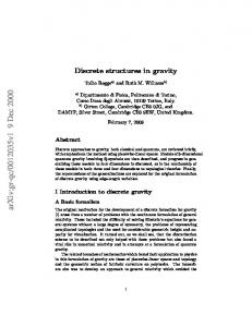
The possibility of particles crossing is introduced on the linear chain by adding fingers of unit length at each site. The corresponding geometrical structure is the narrow comb lattice (NCL) represented in Fig. 2 a. Let us consider two particles starting at t = 0 from the adjacent sites x1 = 0 and x2 = 1 on the backbone of the comb. The particles move on the NCL according to the following rules: i) each particle can jump from site i to one of its nearest neighbors sites with probability 1/zi , zi being the number of nearest neighbors of site i. This means that when a particle is on one of the fingers, it is forced to jump to the backbone with probability equal to one. ii) When the two particles occupy two adjacent sites on the backbone (contact), the particles are forced to move in one of the following ways: a) the two particles jump on the backbone following opposite directions b) both particles jump on the fingers corresponding to their positions c) only one of the particles jumps on the finger while the other moves on the backbone. This can be done in four different ways. Two of them lead to what we shall call a ‘tower configuration’, where the particles occupy a site on the backbone and the site of the corresponding finger. iii) the only allowed evolution of a tower configuration consists in the lower particle taking a further step on the backbone, while the particle on the finger

4

drops down to the backbone. This means that particles have a probability 1/2 to cross each other, depending on the lower particle taking the step to the left or to the right. Now we can build the diffusion graphs for the center of mass cm and the relative distance dr , with cm and dr defined in (1) and (2), where x1 and x2 are the projections on the backbone of the positions of particles 1 and 2 respectively. When one of the particles is on a finger, cm and dr have non integer values and dr has negative values when x1 > x2 . The diffusion graphs of cm and dr are themselves narrow comb lattices, decorated with loops and triangles as in Fig. 3 and Fig. 4. The position of cm on the NCL can be easily deduced from the position of a random walker on the corresponding diffusion graph: when the random walker occupies a site on the backbone, its position corresponds to the value of cm ; when it stays on a finger, the value of cm is that of the position of that finger and both particles occupy sites on the fingers of the NCL. Finally, when the walker is on the upper vertex of one of the triangles, cm has a semiinteger value corresponding to the projection of the vertex on the backbone. In this situation one of the particles is on the backbone and the other on the fingers. Loops are introduced on the diffusion graph of the NCL to represent waiting time probabilities for cm . The relative distance graph can be built in a similar way, taking contact into account. Point O represents the tower configuration which can evolve on point A (contact with x1 < x2 ) or in point A’ (contact with x1 > x2 ) and all the other points will be indicated with the value of their projection on the backbone (1/2, 1, 3/2, 2... and −1/2, −1, −3/2, −2..., depending on the walker being on the left or the right side of the graph with respect to point O). The diffusion graph with the corresponding jumping probabilities is represented in Fig. 4. The jumping probabilities not explicitly indicated are equal to the corresponding ones of the cm diffusion graph. Since points A and A’ represent contacts between particles, we can have particle crossing if A → A’ or A’ → A i.e. crossing can only be the consequence of a contact. Now we can study the motion of the two interacting particles analyzing random walks on the diffusion graphs. The first quantity we calculate is the probability of a contact between particles without crossing. This corresponds to the probability that a single walker starting from point A of the diffusion graph of dr returns to point A after t ′ steps without ever reaching point A′ . We call this quantity P (A ) (A, A; t) and ′ we define F (A ) (A, A; t) as the probability that a walker starting from point A returns to this same point for the first time after t steps without ever reaching point A′ . We have:  ′ 1 1 1 (A) 11 δt,2 + δt,2 + + P (1, 1; t − 2)+ F (A ) (A, A; t) = 32 6 9 6       1 1 1 1 1 1 , 1; t − 2 + P (A) 1, , t − 2 + P (A) , ;t− 2 (3) + P (A) 3 2 2 2 2 2 5

where the first term refers to the two steps A → O → A, the second to the probability of reaching the finger corresponding to point A and then going back to the backbone. P (n) (i, j; t) is the probability of a t steps walk from point i to point j never reaching point n. Let us introduce the generating function of a generic P (n) (i, j; t) as: Pe (n) (i, j; λ) =

∞ X

P (n) (i, j; t)λt

(4)

t=0

Using the relation Pe (n) (i, i; λ) = 1/[1 − Fe (n) (i, i; λ)][16], the calculation of one of the Pe (n) (i, i; λ) is reduced to that of the corresponding Fe (n) (i, i; λ) which is, ′ in general, a much easier task. In the case of F (A ) (A, A; t) we obtain:  ′ λ2 λ2 λ2 1 e (A) Fe(A ) (A, A; λ) = P (1, 1; λ)+ + + 6 6 9 6       1 1 e (A) 1 1 1 e (A) 1 (A) e 1, ; λ + P , 1; λ + P , ;λ (5) + P 3 2 2 2 2 2 The generating functions of Pe (A) (1, 1; λ) and Pe (A) (1/2, 1/2; λ) can in turn be expressed as functions of the corresponding first time generating functions: 2 2 1 Fe (A) (1, 1; λ) = λ 27 1 −

where:

Fe (A)



λ 3

+x

 1 1 1 2 1 , ; λ = λ + λ2 2 2 3 27 1 − x

2 λ2 λ2 + λ+ 9 9 9     2 3 3 1 + Pe (1) , 2; λ + Pe (1) 2, ; λ + 9 2 3 2 x = Fe (A,1/2) (1, 1; λ) =

(6)

(7)



1 e(1) P (2, 2; λ)+ 9   2 e (1) 3 3 P , ;λ 3 2 2

Moreover since Pe(n) (i, j; λ) = Fe(n) (i, j; λ)Pe(n) (j, j; λ) we also have:   λ 1 1 · Pe (A) (1, 1; λ) Pe(A) , 1; λ = 2 1 − λ3 3     1 2λ e (A) 1 1 1 (A) e P · , ;λ 1, ; λ = P 2 1−x 9 2 2

(8)

(9) (10)

Using the translation invariance in the backbone direction of the comb, we get the equalities: Pe (1) (2, 2; λ) = Pe (A) (1, 1; λ); Pe (1) (3/2, 2; λ) = Pe (A) (1/2, 1; λ); 6

Pe (1) (2, 3/2; λ) = Pe(A) (1, 1/2; λ) and Pe (1) (3/2, 3/2; λ) = Pe (A) (1/2, 1/2; λ). We obtain from (8) an equation for x:   λ2 3 + 3λ + 18(1 − x) 2 λ2 x= (11) + λ+ 9 9 9 9(3 − λ)(1 − x) − 2λ2 Now we can substitute the value of x and obtain the final expression:   3 + 3λ + 18(1 − x) λ2 λ2 (A′ ) e 1+ + F (A, A; λ) = 6 6 9(3 − λ)(1 − x) − 2λ2

(12)

′

The asymptotic behavior of P (A ) (A, A; t) can be derived from that of the corresponding generating function considering the limit λ → 1 and then applying Tauberian theorems [16]: r 2 − 32 (A′ ) P (A, A; t) ∼ 12 t→∞ (13) t π

This asymptotic law shows a dramatic difference with respect to the case of the simple linear chain where particle crossing is forbidden and the probability of a contact decays as t−1/2 . Notice that the deep change in the asymptotic behavior, originated by the new geometry, has no analogous if we consider the motion of a single particle, since in this case the linear chain and the NCL have the same asymptotic diffusion laws. In a similar way, we can calculate the probability of particles crossing. This is the probability P (A, A′ ; t) that a random walker starting from point A of the diffusion graph of dr reaches point A′ after a t steps walk. Since Pe (A, A′ ; λ) = Fe (A, A′ ; λ)Pe(A′ , A′ ; λ)

we find after some calculations:

3 P (A, A ; t) ∼ 8 ′

r

2 −1 t 2 π

t→∞

(14)

(15)

A key quantity is the average number of contacts without particles crossing. This is given by the average number of returns to point A after t steps on the dr diffusion graph without reaching point A′ : ′

M (A ) (A, A; t) ∼ const

(16)

Finally, the mean number of particles crossing follows the asymptotic law r 3 2 1 ′ M (A, A , t) ∼ t→∞ (17) t2 4 π For a better description of the diffusion properties of the two particles on the NCL, we study the mean square dispersions ∆x21 and ∆x22 , defined as ∆x21 = ∆x22 =< x21 > − < x1 >2 =< x22 > − < x2 >2 7

(18)

In [3] the mean square dispersions of two hard core interacting particles on a one dimensional lattice was studied. In this case, particle crossing was forbidden by the potential and by the geometry of the system and it was found that   1 2 2 ct (19) ∆x1 = ∆x2 = 1 − π c being the diffusion constant, while for a single particle moving freely on a one dimensional lattice we have ∆x21 = c t (20) From the previous results it follows that the interaction inhibits through the factor (1 − 1/π) the spreading. In the NCL case, from (1) and (2) it follows that: < x1 >=< cm − dr > (21) < x2 >=< cm + dr > +1

(22)

The expressions of < cm > and < dr >, due to the diffusion graph transform, can be calculated as the mean displacement < d > of a single walker moving on the correspondent diffusion graph, d being the coordinate of the projection of the position of the walker on the backbone of the diffusion graphs. Using the equation P∞ d P (O, d; t) < d >= P−∞ (23) ∞ −∞ P (O, d; t)

and following the steps described in [17] we find < cm >=< dr >= 0: this also immediately follows from the fact that the diffusion graphs of cm and dr are symmetric with respect to point O so that < cm > and < dr > must be 0. Equations (21) and (22) become < x1 >=< cm − dr >= 0

(24)

< x2 >=< cm + dr > +1 = 1

(25)

∆x21 = ∆x22 =< c2m > + < d2r >

(26)

and we have also By straightforward calculations we find < c2m >∼

1 t 4

t→∞

(27)

< d2r >∼

1 t 4

t→∞

(28)

so that ∆x21 = ∆x22 ∼ 8

1 t 2

t→∞

(29)

For a single particle diffusing on the NCL we have ∆x2 ∼

1 t 2

t→∞

(30)

where x is defined as the projection of the particle position on the backbone of the lattice (for a single walker on a linear chain ∆x2 ∼ t t → ∞). We can therefore conclude that the interaction between particles does not modify the spreading as a consequence of the possibility of particle crossing. This result is confirmed by equations (13) and (15), stating that a contact with crossing is much more frequent than a contact without crossing.

4

Two interacting particles on ladder lattices

The ladder lattice exhibits new features with respect to the previous cases due to the presence of loops. The ladder graph is made of two linear chains whose corresponding points are connected by links as in Fig. 2 b. The two particles start from the same site and then move on the ladder with jumping probabilities equal to 1/3. The relative distance is defined as dr = N/2, N being the chemical distance i.e. the number of links of the shortest path connecting the two particles. The dr diffusion graph is represented in Fig. 5; the value of dr is given by the projection on the lower chain of the position of a random walker. When the walker is on the lower chain of the dr diffusion graph, particles on the real ladder lattice are on the same chain, while when the walker jumps on the upper chain of the dr diffusion graph it means that particles move on different chains. Point O represents the contact between particles and the link between A and A′ represents the possibility of particles crossing each other without direct contact, since it connects points with dr > 0 and dr < 0 without passing through point O. This is the direct consequence of the presence of loops and it represents a fundamental technical difference with respect to the previous case. The solution of the random walks problem on the diffusion graph can be simplified by the following considerations. As already shown in [18] the diffusion problem on a ladder-like lattice can be mapped into that of a linear chain. This follows from the fact that we are interested only in the walker displacement in the unbounded direction, and not in its position on the upper or on the lower chain. Then the ladder can be considered as a linear chain where we define additional staying probabilities corresponding to the steps spent for jumping from one chain to the other. In the present case this simplification can be applied to the two half-linear chains originating from the central loop. Notice that the central loop cannot be reduced to a couple of points of the linear chain and must survive our transformation since it breaks the translational symmetry of the network. This detail is crucial for the calculation of crossing without contact probability. The final graph obtained by this analysis is represented in Fig. 6. It reproduces 9

the main features of the dr diffusion graph for the probability of particles crossing with or without contact. From calculations analogous to the previous case we find that the probability of contact without crossing is: r 36 2 − 3 (A′ ) t→∞ (31) P (A, O; t) ∼ t 2 25 π and shows the same time dependence we found in the NCL case. The probability of crossing without contact is: r 48 2 − 3 (O) ′ t→∞ (32) t 2 P (A, A ; t) ∼ 25 π while the generic probability of crossing decays as: 3 1 P (A, A′ ; t) ∼ √ t− 2 2π

t→∞

(33)

The description of the steps leading to (31), (32), (33) can be found in Appendix A. We see that the probability of a contact without crossing on the ladder lattice follows the same law we found in the NCL case and this is also true for the crossing probability. On the ladder lattice however, a probability of crossing without contact can be defined. This particular feature of the ladder lattice can be extremely useful when the two processes representing contact and crossing are used to represent different physical situations.

5

Summary and Discussion

The diffusing graph transform introduced in this paper is a powerful technique which, combined with the universality properties of the long time asymptotic behavior of random walks return probabilities, provide a new tool for the analysis of interacting diffusing particles on discrete structures. The technique can be applied to decouple and analytically solve the problem on tree-like and quasi 1-dimensional structures also in presence of loops and crossing probabilities for the particles. This has been done for the case of two interacting particles on the Narrow Comb and on the Ladder lattice. Our solution shows that the asymptotic behavior of contact probabilities is sensitive to the local geometrical details of the underlying discrete structure.

Appendix A The explicit calculation of (31), (32), (33) is based on two properties of the generating functions [16]. The first states that the generating function of the 10

probability Pe (k) (i, j; λ) of going from point i to point j (i 6= j), without ever touching point k, is related to the corresponding first time arrival generating function by the relation Pe (k) (i, j; λ) = Fe (k) (i, j; λ) · Pe (k) (j, j; λ)

(A.1)

The second property is the well known relation between Pe (k) (i, i; λ) and Fe(k) (i, i; λ) we already used in the preceding sections; Pe (k) (i, i; λ) =

1 (k) e 1 − F (i, i; λ)

(A.2)

′ Let us start from the calculation of Pe (A ) (A, 0; λ): from (A.1) it follows that:

since:

′ ′ ′ Pe(A ) (A, 0; λ) = Fe (A ) (A, 0; λ) · Pe (A ) (0, 0; λ) ′ ′ λ Fe (A ) (A, 0; λ) = Pe (0,A ) (A, A; λ) 6

and ′ Pe (A ) (0, 0; λ) =

1 = (A e 1 − F ′ ) (0, 0; λ) 1−

1 λ2 e (O,A′ ) (A, A; λ) 12 P

(A.3)

(A.4)

(A.5)

′ ′ so that the calculation of Pe (A ) (A, 0; λ) is reduced to that of Pe (O,A ) (A, A; λ). ′ To obtain the expression of Pe (O,A ) (A, A; λ) we calculate the corresponding first time arrival generating function: ′ 5λ Fe (O,A ) (A, A; λ) = + 9



2λ 9

2

Pe (A) (1, 1; λ)

(A.6)

From the translational invariance of the lattice, we have that Pe(A) (1, 1; λ) = ′ Pe (O,A ) (A, A; λ). Using the preceding relation together with (A.2) we obtain: q 2 5λ 1 + λ9 − 10λ 1 − − ′ 9 9 (A.7) Pe (O,A ) (A, A; λ) 8λ2 81

In the limit λ → 1 − ǫ and ǫ → 0 we have:

and:

′ 9 Pe (O,A ) (A, A; 1 − ǫ) ∼ 2

r   ǫ 1−3 2

′ 6 72 √ 2ǫ Pe (A ) (A, 0; 1 − ǫ) ∼ − 5 25

11

(A.8)

(A.9)

Applying Tauberian theorems we obtain (31). For the determination of Pe(O) (A, A′ ; λ), ′ we follow the same technique writing this quantity as a function of Pe (O,A ) (A, A; λ), taking the limit λ → 1 − ǫ(ǫ → 0) and using Tauberian theorems. In conclusion we have: λ e (O,A′ ) P (A, A; λ) (A.10) Fe (O) (A, A′ ; λ) = 18  2 ′ 1 λ Fe (O) (A′ , A′ ; λ) = 1 − + Pe (O,A ) (A, A; λ) (A.11) ′) (O,A e 18 P (A, A; λ) and finally using (A.2) we have

Pe(O) (A, A′ ; λ) = Fe (O) (A, A′ ; λ) · Pe (O) (A′ , A′ ; λ)

(A.12)

Pe (A, A′ ; λ) = Fe (A, A′ ; λ)Pe(A′ , A′ ; λ)

(A.13)

For Pe (A, A′ ; λ) the corresponding steps can be resumed as: Fe(A′ , A′ ; λ) = 1 − 

1 + ′) (O,A e P (A, A; λ)

 1 e (O,A′ ) λ e(O,A′ ) P (A, A; λ) + P (A, A; λ) + 1 9 12 − λ2 Pe(O,A′ ) (A, A; λ) 27 (A.14)   e(O,A′ ) (A, A; λ) P 2λ (A.15) + λ2 Fe (A, A′ ; λ) = 12 − λ2 Pe (O,A′ ) (A, A; λ) 3 λ2

References

[1] T. E. Harris, J. Appl. Prob. 2, 323 (1965) [2] M.E. Fisher, Jour. of Stat. Phys., 34, 669, (1984) [3] C. Aslangul, Eur. Lett., 44 , 284, (1998) [4] C. Aslangul, Cond. Mat. 9902142 (1999) [5] C. Aslangul, J. Phys. A, 32, 3993, (1999) [6] M. Bauer, C. Godreche,J.M. Luck, Cond. Mat. 9905252, to appear in Jour. Stat. Phys., (1999) [7] J.W. Essam and A.J. Guttmann, Phys. Rev. E 52 5849-5862, (1995) [8] D.K. Arrowsmith, P. Mason and J.W. Essam, Physica A, 177, 267-272, (1991)

12

[9] C. Krattenhaler, A. Guttmann and X. Viennot, Cond. Mat. 0006367, (2000) [10] J.W.Cahn, Jour. Chem. Phys. , 66, 3667, (1977) [11] P.M Richards, Phys. Rev. , B 16, 1393, (1977) [12] V. Kukla, J. Kornatowsky, D. Demuth, I. Girnus, H. Pfeifer, L.V.C. Rees, S.Schunk, K.K. Unger, J. Karger Science, 272, 702, (1996) [13] E. Nener, Science, 256, 498, (1992) [14] B. Sackman, Science,256, 503, (1992) [15] G. Giusiano, Diffusione di Particelle interagenti su strutture a bassa dimensionalit` a, Tesi di laurea Universit` a di Parma, (1999) [16] E.W. Montroll and G.H. Weiss, Jour. of Math. Phys., 6, 167, (1965) [17] D. Cassi Eur. Lett. 9, 627, (1989) [18] S.Revathi, V.Balakrishnam, Phys. Rev. E 47, 916, (1993)

13

Figure captions

Fig.1 The diffusion graphs of a linear chain: a) cm diffusion graph and b) dr diffusion graph Fig.2 a) ‘Truncated comb lattice’ b) ‘Ladder lattice’ Fig.3 cm diffusion graph and jumping probabilities for the truncated comb lattice Fig.4 dr diffusion graph and jumping probabilities for the ‘Truncated comb lattice’ Fig.5 dr diffusion graph and jumping probabilities for the ‘Ladder lattice’ Fig.6 Semplified dr diffusion graph for the Ladder lattice

14

1

a)

2

1 0 0 1

1 0 0 1

1 0 0 1

1 0 0 1 1 4

O

11 00 00 11

1 0 0 1

1 0 111111 000000 0 1

1 4

1

b)

2

1

11 00 00 11

O

1 0 0 1

1 0 0 1

1

1

4

4

1 0 0 1

11 00 00 11

1 0 0 1

11 00 00 11

1 0 0 1

1 0 0 1 00 11 00 11 00 11 0 1 0 1 0 1 00 11 0 1 0 1 0 1 0 1 0 1 0 1 0 1 0 1 0 1 0 1 00 11 00 11 00 11 0 1 0 1 0 1 00 11 1 1 1 1 1 1 1 1 0 0 0 0 0 0 0 0 0 1 0 1 00 11 00 11 00 11 0 1 0 1 0 1 00 11 1 1 1 1 1 1 1 1 0 0 0 0 0 0 0 0 0 1 0 1 0 1 0 1 0 1 0 1 0 1 0 1 0 1 0 1 0 1 0 1 0 1 0 1 0 1 0 1 1 1 1 1 1 1 1 1 0 0 0 0 0 0 0 0 0 1 0 1 0 1 0 1 0 1 0 1 0 1 0 1 1 1 1 1 1 1 1 1 0 0 0 0 0 0 0 0 0 1 0 1 0 1 0 1 0 1 0 1 0 1 0 1 1 1 1 1 1 1 1 1 0 0 0 0 0 0 0 0 0 1 0 1 00 11 00 11 00 11 0 1 0 1 0 1 00 0000 11 11111 00000 111111111111111111111111111111111111111111 000000000000000000000000000000000000000000 1111 1 1 1 1 1 1 1 1 0 0 0 0 0 0 0 0 0 1 0 1 00 11 00 11 00 11 0 1 0 1 0 1 00 11 0 1 0 1 00 11 00 11 00 11 0 1 0 1 0 1 00 11

a) 0 1 0 1 00 11 00 11 00 11 0 1 0 1 0 1 00 11 00000 11111 111111111111111111111111111111111111111111 000000000000000000000000000000000000000000 0 1 0 1 0 1 0 1 0 1 0 1 0 1 0 1 11111 00000 11 00 0 1 0 1 00 11 00 11 00 11 0 1 0 1 0 1 00 11 0 1 0 1 0 1 0 1 0 1 0 1 0 1 0 1 0 1 0 1 00 11 00 11 00 11 0 1 0 1 0 1 00 11 0 1 0 1 0 1 0 1 0 1 0 1 0 1 0 1 1 1 1 1 1 1 1 1 0 0 0 0 0 0 0 0 1 1 1 1 1 1 1 1 0 0 0 0 0 0 0 0 0 1 0 1 0 1 0 1 0 1 0 1 0 1 0 1 0 1 0 1 0 1 0 1 0 1 0 1 0 1 0 1 0 1 0 1 0 1 0 1 0 1 0 1 0 1 0 1 1 1 1 1 1 1 1 1 0 0 0 0 0 0 0 0 0 1 0 1 0 1 0 1 0 1 0 1 0 1 0 1 0 1 0 1 0 1 0 1 0 1 0 1 0 1 0 1 0 1 0 1 00 11 00 11 00 11 0 1 0 1 0 1 00 11 11111 00000 111111111111111111111111111111111111111111 000000000000000000000000000000000000000000 1111 0 1 0 1 00 11 00 11 00 11 0 1 0 1 0 1 00 0000 11

b)

1 3

1 0 0 1 0 1

11 00 00 11 00 11 1 0 0 1

1 0 0 1 0 1

2 9

1 0 0 1 0 1

1 3

2 9

11 00 00 11 11 00 00 11

1 9

11 00 00 11

O

11 00 00 11

1 9

1 0 0 1 0 1

11 00 00 11

11 00 00 11 00 11

11 00 00 11

1 0 0 1

O 1 0 0 1 0 1

11 00 00 11 00 11

-1

11 00 00 11 00 11

1 2

11 00 00 11 00 11

11 00 00 11 00 11 11 00 00 11 00 11

A’

1 3

1 3

1 0 0 1 0 1

A

1 0 0 1 0 1

1 0 0 1 0 1

1 6 1 6

11 00 00 11 00 11

1

11 00 00 11 00 11

1 3

11 00 00 11 00 11

1 0 0 1 0 1

00 A11 00 11 00 11

A’

1

1

9

9

1 0 0 1 0 1

2 9

9

2

1 3

11 00 00 11

1 3

O

1 0 0 1

1 0 0 1

1

9 2

9

9

11 00 00 11

1

1

6

6

1 9

1 3

2

1 0 0 1

2 18

2

11 00 00 11

9

-111 00 00 11

11 00 00 11

A’ 00 11 00 11

1 2

11 00 00 11

2

2

1

9

9

6

5

5

9

9

O

A 11 00 00 11

1 11 00 00 11

11 00 00 11

11 00 00 11