Two Matlab Functions for Understanding How Fast Fourier Transform Works Zhigang Xu (
[email protected]) Maurice Lanmontagne Institute Department of Fisheries and Oceans Canada 2013/Oct/03
Summary Two m-functions, sfft and sifft, are supplied as plain text counterparts to the Matlab binary built-in functions of fft and ifft. You can not only read their codes but also can step through their executions. The accompanied document derives and explains the Cooley-Tukey fast Fourier transform (FFT) algorithm. The programs and the document should be helpful to those who want clearly understand how the FFT works. The m-files can be downloaded from the mathworks file exchange center.1
Contents 1.
Introduction ........................................................................................................................................... 1
2.
Fourier Matrix, Discrete Fourier Transform (DFT) and its Inverse (IDFT) ......................................... 2
3.
Properties of wn e
4.
FFT Algorithm ...................................................................................................................................... 6
5.
Fourier Matrix Factorization ................................................................................................................. 9
6.
FFT on a Binary Tree ............................................................................................................................ 9
7.
SFFT and SIFFT, Text Counterparts of FFT and IFFT .................................................................... 12
8.
References:.......................................................................................................................................... 15
1.
1
2 i n
, Fast Fourier Transform, FFT and IFFT ....................................................... 4
Introduction
http://www.mathworks.ca/matlabcentral/fileexchange/?search_submit=fileexchange&query=sfft&term=sfft
1
Matlab has fft and ifft already to fast calculate discrete Fourier transform and it inverse. However they are binary built-in functions, hence their code is not visible, which is not helpful to someone who wants to understand how FFT works. For teaching and learning purposes, I think we should also have a pair of their readable counterparts, written and stored in plain text (the so-called the Matlab m-functions), which we can step through during their executions. I searched Mathworks file exchange center but did not find any one had contributed such m-functions. Therefore I hope that this contribution will be welcome to the Matlab user community. To avoid name conflicts, I name my pair of functions sfft and sifft. Using letter s as a prefix is learnt from Professor Gilbert Strang (Ref. 1) in MIT, who presented slu as readable counterpart to the Matlab builtin function lu for lower and upper triangular matrix factorization. I do not know why he chose s at the first place. Perhaps it was derived from the word script, something written in text.2 The contents of this article are more than its title suggests. I am sorry that I could not come up with a better title! The contents consist of more mathematics and algorithm of FFT than of the functions themselves. The best way to understand the functions is to understand their mathematical background. Presentation of the functions becomes much easier after presenting the mathematics and algorithm behind them. I will try my best to explain them in an easy-to-follow manner. If your original understanding about
n log 2 n number of multiplications instead of n 2 , this 2 n article will tell you that the actual number of multiplications is even less; it is (log 2 n 1) . The 2 FFT is that it goes fast because it only requires
butterfly diagram is a traditional choice to graphically explain the FFT algorithm. You will see the butterfly diagrams in most textbook. If you google with the key words “butterfly + FFT”, you will hit many pages. In this article I choose a different visual aid, the binary tree borrowed from the computer science, to explain the algorithm. Hope you will like this alternative. If you have any comments, please email me.
2.
Fourier Matrix, Discrete Fourier Transform (DFT) and its Inverse (IDFT)
An nth-order Fourier matrix, Fn , is a square matrix with entries given by
Fn ( j, k ) e
2 i jk n
,
with j, k 0,1,2,
,n 1
(1)
Take n=4 as an example, we can see F4 in a little nice square
2
So do not be confused with the special meaning of “script” assigned by Matlab. Matlab distinquishes between a
script and a function: a script is an external file that contains a sequence of MATLAB statements; a function has inputs and outputs and function declaration. The sfft and sifft are functions.
2
1 1 1 1 1 2 3 4 4 4 F4 2 4 1 4 4 46 3 6 9 1 4 4 4
(2)
where
4 e
i
2 4
i
(3)
The indices for the rows and the columns are from 0 instead of 1. The 0-based indexing is convenient for the discrete Fourier transform. It is called a Fourier matrix because it can convert an n-point data sequence into a harmonic frequency based sequence. For example, a 4-point data sequence, xk (k 0,1, 2, 3) , can be converted to four harmonic amplitudes, c j (j 0,1, 2, 3) , simply by its multiplication with the data vector
1 1 x0 c0 1 1 c 1 2 3 x 4 4 4 1 1 2 4 c2 1 4 4 46 x2 3 6 9 c3 1 4 4 4 x3
(4)
The c j (j 0,1, 2, 3) are also called the Fourier coefficients. They are complex valued, containing information of both amplitudes and phases of the harmonic oscillations. A property of the Fourier matrix is that they are column orthogonal:
FnH Fn nI
(5)
where FnH denotes the conjugate transpose of Fn and I is the nth-order identity matrix. Using this property, the data in physical space can be reconstructed with Fourier coefficients by.
x0 1 1 x 1 w 4 1 1 x2 4 1 w42 3 1 w4 x3 where w4 4 e
2 i 4
1 w42 w44 w46
1 c0 w43 c1 w46 c2 w49 c3
(6)
.
For an arbitrary n-point data sequence, we have the following pair of discrete Fourier transforms:
3
c Fx
x
(7)
1 H F c n
(8)
They transform the information between the time (or space) domain and the frequency (or wave number) domain. Although the two transforms are inverse to each other, customarily eq. (7) is called the discrete Fourier transform (dft) and the eq. (8) is called the inverse discrete Fourier transform (idft). Earlier versions of Matlab (versions 2, 3, or even earlier) included two m-functions, dft and idft, which carry out the Fourier matrix-vector multiplications in a for-loop. Let me quoted them here so that you can see how Eqs. (4) and (4) are implemented and later you can also compare them with their fft counterparts.
function y = dft(x) %DFT DFT(X) is the discrete Fourier transform of vector X. % See also IDFT, FFT, IFFT. % J.N. Little 11-25-85 % Copyright (c) 1985, 1986 by the % MathWorks, Inc.
function y = idft(x) %IDFT IDFT(x) is the inverse discrete Fourier transform of X. % See also DFT, FFT, IFFT.
n = max(size(x)); Wn = exp(-1i*2*pi/n); y = x; N = 0:n-1; for k=1:n y(k) = Wn.^((k-1)*N) * x(:); end
n = max(size(x)); Wn = exp(-1i*2*pi/n); y = x; N = 0:n-1; for k=1:n y(k) = Wn.^((1-k).*N) * x(:); end y = y / n;
Table 1 Two discrete Fourier transform functions, dft and idft, from earlier version of Matlab
3.
Properties of wn e2 i / n , and Fast Fourier Transform, FFT
With aid of eq (4), or from the functions in Table 1, we can easily see that to compute a n-point dft requires n 2 multiplications (and (n 1)2 number of additions, but we count the multiplications only for a measure of computational load). However Cooley and Tukey (1965) invented an ingenious algorithm which can compute the same Fourier transforms but only with
1 2
n log 2 n number of multiplications. Their
algorithm has been named as Cooley-Tukey FFT and IFFT. The FFT stands for fast Fourier transform, and the IFFT stands for its inverse. Properties of wn e2 i / n
4
The little element wn e2 i / n (and n e2 i /n as well) has some properties that play critical roles in the FFT algorithm. The wn is one of the roots of equation z n 1 . Take n=4 for example again, there are four roots, w4k (k 0,1,2,3) , distinct and equally distributed along a unit circle (Figure 1) with 90-degree angle apart from each other.
Any w4k with k>3 is also a root, but not distinct from the four basic ones
( w40 , w41 , w42 , w43 ) . As shown in the figure, w44 and w48 are the same as w40 , w45 and w49 are the same as
w41 , and so forth. In fact, any higher powers of w4 just cycle through the four basic roots. Around a circle, everything is periodic in 2𝜋, which makes wnk periodic in n:
wnk n wnk , (periodicity property)
(9)
because k n n
w
e
2 i ( k n ) n
e
2 i k 2 i n
e
e
2 i k n
wnk
(10)
Figure 1 Four basic roots of z 4 1 are equally spaced along a unit circle, they are w40 , w41 , w42 , and w43 with w4 e2 i /4 . Higher powers ( 4 ) of w4 are also the roots but cycle through the basic ones. The roots at the opposite ends of the same diameters are negative to each other. w40 and w42 are also the roots of z 2 1 , which equal to w20 and w21 .
5
The four basic roots are located at the ends of the two diameters. The roots paired by the same diameter have opposite signs, because their angles differ by . Generally, when n is a non-zero and even number, we can have n/2 diameters to pair the roots, (w kn , wnk n /2 ) , negative to each other:
wnk wnk n /2 ,
k 0,1, 2,
(11)
, n / 2 - 1, (skew symmetry property)
because
w e k n
2 i k n
i
e e
2 i k n
e
2 i ( k n /2) n
wnk n /2
(12)
This is another key property that the FFT algorithm is based on. This property is called the symmetry property in some texts (e.g, Ref 2), but I think to call it a skew symmetry property may be more appropriate, because this way we also convey the negative sign. The four basic roots are the elements of the 1st column (again, the counting here is 0-based) of the Fourier matrix, F4 . The elements in the 2nd column are w40 w44 1,and w42 w46 1 , distributed at the ends of the horizontal diameter.3 They are also the roots of z 2 1 , which are w20 1 and w21 1 . This leads us to the third property,
wn2k wnk/2 ,
n=2,4,6, , (connectivity property)
(13)
This is because
wn2 k e
2 i 2k n
2 i
e n /2
k
(14)
This property connects a higher order Fourier matrix to a lower one. I do not know if it has had a proper name already, but let me call it here a connectivity property. With it, we can connect Fn to Fn /2 . If
n 2l , we can recursively connect Fn to F1 in l steps. The properties of periodicity, skew symmetry and connectivity also hold for n k e
2 i k n
, which are also
the roots of z n 1 , but going around the unit circle clockwisely.
4.
3
FFT Algorithm
We may view the horizontal diameter an even-numbered diameter (the 0th diameter) and the vertical one an odd-
numbered diameter (the 1st diameter). When the basic roots
( w40 , w41 , w42 , w43 ) are raised to a 2nd power
( w40 , w41 , w42 , w43 )2 , or to any even-numbered power, those of the basic roots that are located at the ends of the oddnumbered diameters will be all relocated to the end of the even-numbered diameters.
6
Now we are ready to go for the FFT algorithm. Let us take the matrix-vector multiplication on the RHS of eq. (4) as an example and go through the following derivations step by step to see how the three properties highlighted above can help us to reduce the number of multiplications to
n log 2n from n 2 2
otherwise:
1 1 x0 x0 1 1 x 1 2 3 x 4 4 4 1 F4 1 2 4 x2 1 4 4 46 x2 3 6 9 x3 1 4 4 4 x3
(15)
1 1 1 1 1 2 x 3 x 4 0 4 1 = 42 4 1 4 x2 4 46 x3 3 6 9 1 4 4 4
(even-odd splitting)
(16)
1 1 1 1 1 1 2 x 1 2 x 4 0 4 4 1 = 4 2 4 1 4 x2 1 44 x3 6 43 1 46 1 4
(factoring)
(17)
1 1 1 1 1 1 2 x 1 2 x 4 0 4 4 1 = 2 4 1 1 x2 1 1 x3 2 43 1 42 1 4 1 1 1 1 1 1 x 1 x 2 0 4 2 1 = 2 4 1 1 x2 1 1 x3 43 1 2 1 2
1 1 1 1 x 2 0 4 = 1 1 x2 1 2
1 1 1 x 2 1 1 1 1 x3 4 1 2
(periodicity
nk n nk )
(18)
(connectivity
wn2k wnk/2 )
(skew symmetry
nk n /2 nk )
(19)
7
1 1 1 1 1 x 4 1 1 x1 0 = 1 2 x3 1 1 2 x2 1 4 1 1 1 1 x 4 x1 F2 F2 0 = x3 1 x2 1 4 1
( F2
F2x even D2F2x odd F2x even D2F2x odd
1 1 1 2
(20)
(21)
definition of Fourier matrix)
( D2
=
where a new symbol
(factoring)
1 4
(22)
new symbol)
D 2 has been introduced to denote the diagonal matrix diag (1, 4 ) . In general,
Dn /2 diag (1, n , n2 ,
, nn /21 ) with even n.
Thus a 4th order matrix-vector multiplication has been reduced to two of 2nd order matrix-vector multiplications,
F x D2F2x odd F4x 2 even F2x even D2F2x odd where
x [ x0 x1 x2 x3 ]T and x even and x odd are its sub-column vectors with even and odd indices respectively.
For the two multiplications of
where
(23)
F2 times vectors, we can apply the same decomposition:
F x D1F1 x2 x0 x2 F2x even 1 0 F1 x0 D1F1 x2 x0 x2
(24)
F x D1F1 x3 x1 x3 F2xodd 1 1 F1 x1 D1F1 x3 x1 x3
(25)
F1 1 and D1 1 by their definitions.
For the Fourier matrix order one,
Fn when n is an even number, we can follow the same procedure to connect it to a lower
Fn /2
8
I D Fn x n /2 Fn/2x even n /2 Fn /2x odd I n /2 Dn /2 where
(26)
I n /2 is an identity matrix of order n/2, x even and x odd are two sub-sequences extracted from x with even
and odd indices respectively, and
Dn /2 is a diagonal matrix with (1, n , n2 ,
, nn/21 ) as its diagonal entries. If
n 2l (l 1,2,3, ) , we can recursively connect Fn to F1 in l steps. I postpone counting of number of the multiplications after I link FFT to a binary tree.
5.
Fourier Matrix Factorization
From eq. (26) we can further derive a Fourier matrix factorization formula,
I D Fn x n /2 Fn/2x even n /2 Fn /2x odd I n /2 Dn /2 Dn /2 Fn /2 I n /2 Px Fn /2 n I n /2 Dn /2
(27)
from which we have the factorization,
I Fn n /2 I n /2
Dn /2 Fn /2 Dn /2
P Fn /2 n
(28)
where Pn is an nth-order permutation matrix for the needed even and odd permutation.
6.
FFT on a Binary Tree
Eq. (26) suggests that FFT is a recursive algorithm. To see graphically how the information flows during the recursion, a butterfly diagram is often used, which consists of a set of horizontal and diagonal lines for information pathways. (e.g., http://en.wikipedia.org/wiki/Butterfly_diagram). Here let me take a different visual aid, a binary tree borrowed from computer science, to see how the FFT works. A tree consists of nodes and edges as illustrated in Figure 2, where the nodes are shown as rectangular boxes and the edges are shown as the lines connecting the nodes. I have labelled the nodes with the some key contents to indicate what the nodes will do when the information flow reaches there. I have also put the arrows at the tip of the edges to indicate directions of the information flow. There should be arrows at the two ends of each edge, since the information comes in has to go back later on through the same edge. However I have split the same tree into two versions. The version of the left side of the figure focuses on the downwards information flow and the one on the right side focus on the upwards flow. I have also 9
labelled the same nodes differently in the left and in the right versions, to indicate what the main things nodes will do when information flows in and when the information flow returns. Without such splitting, the labels would be all jammed together.
Figure 2 The FFT algorithm can be explained by a binary tree. For clarity, the tree is presented in two versions, the version on the left focus on the tree traversal from top to bottom and the version on the right focus on the traversal from the bottom to the top. The numbers in the parentheses along the tree edges indicate the step numbers of the tree traversal. The traversal is interwoven between the left and the right versions of the tree.
A complete and full binary tree has a node at the top as the tree root. The root has two child nodes (the left child and right child) and each child has two children too, except those at the bottom where nodes no longer have children. Nodes without children are called leaves. Nodes have depths, measured by the number of edges from the nodes to the root. A non-leaf node can also be the root of a subtree which links all the nodes beneath it. Figure 2 is designed to show how the FFT algorithm recursively calculate the multiplication of the 4th order Fourier matrix, F4 times a 4-point vector x [ x0 x1 x2 x3 ]T . Let us begin our FFT journey starting from the root node at the left. The content of the root node shows a function call, F4 ( x0 , x1, x2 , x3 ) . Here I use “F” to stand for a function and its subscript 4 means it takes in a 4-point data. Evidently, F4 also closely resembles F4 of the 4th order Fourier matrix, indicating that the return from this function should be the result of F4 multiplying with the vector [ x0 x1 x2 x3 ]T . Upon receiving an input, the function will first detect the length of the input. If the length is greater than one, it will split the input into two halves, an even-indexed half, ( x0 , x2 ) , and an odd-indexed half, ( x1 , x3 ) , and then call the function itself (the so-called recursive function call) with the two halves respectively. To guide us where to go next, we follow a rule for tree traversal known as the-left-and-depth first. According to this rule, the even-indexed half is first passed to the left child (arrow 1). The odd-indexed half is not passed to the right child at this moment; it has to wait until the root receives a return from its left child. When the 10
left child receives the 2-point data input, it splits the input into two halves too. Now the even half contains only x0 and the odd half is only x2 . The 1-point even half is passed to its left child (arrow 2), where the bottom of the tress is reached, and the input cannot be split anymore. The function F1 there is very simple, it simply copies x0 as its output (the 1st-order Fourier matrix is 1!). The output is then returned to the parent node (arrow 3). Having received the return from its left child, the parent now can issue the 1-point odd half, x2 , to its right child (arrow 4). The right leaf node also simply copies the input as its return to the parent (arrow 5). Having received the returns from its both children, the parent now can assemble the returns according to the matrix formula indicated by the content of the parent node. The assembled result is then returned to the root node (arrow 6). Having received the return from its left subtree, the root can now release the odd half data ( x1 , x3 ) to let it traverse the right subtree (arrow 7). The right subtree traversal repeats the same procedure as the left subtree traversal (arrows 7 to 12). The root assembles the returns from its left subtree and the right subtree and completes the calculation of the multiplication the matrix with the vector F4 x . Now it is time to count the number of multiplications. The nodes at the depth immediately above the bottom can be also viewed as roots of subtrees. Each of the subtrees has two leaves, the left and the right leaves. The leaf nodes do not need any multiplications; all the operations there are simply copying the inputs as the outputs. When the leaf nodes return their outputs, each of their parent nodes need a multiplication of D1 times the return from its right child. For example, the root of the left subtree shown in the right side of Figure 2 needs a multiplication of D1 times x2 and the root of the right subtree has to multiply D1 with x3 . At this depth, there are 2l1 parent nodes, each of which needs 1-multiplication, so the total number of multiplications is 2l1 . At the next depth up, each of the nodes there needs to multiply D 2 with the return from its right child. There are only 2 nonzero elements in diagonal matrix D 2 and there are two elements in the return from the right child. Therefore it takes 2 multiplications to compute D2xodd . There are 2l2 nodes at this depth, and each node needs 2 multiplications, making the total multiplications still be 2l1 . At the next depth up, there are 2l3 nodes but the D4xodd requires 4multiplications, so the total number of multiplications is still 2l1 . Continue this analysis, you will find that all the depths (except the very bottom) share the same number of multiplications. At the very top, where there is only one node (the tree root), however the Dn /2xodd needs n / 2 2l 1 multiplications. From the root to the depth just above the leaves, there are l depths. So the total number of the multiplications through the whole tree is 2l 1 l
n n l log2 n . 2 2
Actually the count could be still less. If we notice that D1 1 , we can skip all the multiplications at the depth of 2l1 . This makes the number of multiplications become
n (l 1) . I will take this advantage in 2
coding my version FFT and IFFT functions.
11
7.
SFFT and SIFFT, Text Counterparts of FFT and IFFT
Shown in Table 2 is Matlab code for sfft, which has its sub-function called recur_sfft. The main function serves as a user interface to allow for different formats of inputs. Row or column vectors, or matrix inputs are allowed. When the length of an input is not equal to a power of 2, zeros will be padded to the input to increase its length to the next power of 2. The sub-function carries out the iterative calculations. There is also a global variable, count, to count the number of multiplication. function [c, count]=sfft(x) % sfft: Readable text version of fft to fast calculate the discrete % Fourier transform of the input x. % % Input: x, can be a vector (row or column) or matrix. When x is % matrix, the Fourier transform is performed columnwise. % The length of x is expected to be a power of 2. If not, % zeros will be padded to the end of x to increase its length % the next power of 2. Multidimensional array inputs are not % supported. % % Output: c, the complex Fourier coefficients. Its preserves the % dimensions of the x when zero-padding is not applied to x. % If zero-padding is applied, c will be longer or taller % than x. % % Also see sifft. % % Zhigang Xu, 2013/Sept/29 1. 2. 3. 4. 5. 6. 7. 8. 9. 10. 11. 12. 13. 14. 15. 16. 17. 18. 19. 20. 21.
global count
% for counting the number of multiplications.
%% Prepare for the recursive call. count=0; zeropad=false; [siz1 siz2]=size(x); if siz1==1 % x is a row vector n=siz2; ell=log2(n); if mod(ell, 1)~=0, ell=ceil(e); n=2^ell; x(end+1:n)=0; zeropad=true; end x=x(:); % recur_sfft requires a column vector. c=recur_sfft(x); c=c.'; else % x is a column vector or matrix n=siz1; ell=log2(n); if mod(ell, 1)~=0,ell=ceil(e); n=2^ell; x(end+1:n,:)=0; end c=recur_sfft(x); end
12
22. 23. 24. 25. 26. 27. 28. 29. 30. 31. 32. 33. 34. 35. 36. 37. 38. 39. 40. 41. 42. 43. 44. 45. 46. 47. 48. 49. 50. 51. 52.
if zeropad warning('The input has been zero-padded to increase its length to the next power of 2.') end
function c=recur_sfft(x) global count n=size(x,1); if n>2 c_even=recur_sfft(x(1:2:n,:)); % (0:2:n-1)+1 c_odd=recur_sfft(x(2:2:n,:)); % (1:2:n-1)+1 % even means (0:2:n-1),and odd means 1:2:n-1 but they need to be added by 1 to meet Matlab's 1-based indices. k=1:n/2; w=exp(-pi*2i/n); D=spdiags(w.^(k-1).', 0, k(end), k(end)); c_odd=D*c_odd; count=count+k(end)*size(c_odd,2); % counting number of multiplications % fill in the second half of c first c(k+n/2,:)=c_even-c_odd; % which has also pre-allocated RAM for the first half of c % now do the first half of X. c(k,:)=c_even+c_odd; else % the bottom is reached, 2-point of x. c=[x(1,:)+x(2,:) x(1,:)-x(2,:)]; end
Table 2 Function sfft, a text version of the Matlab built-in function fft, to understand how the Cooley-Tukey fast Fourier transform algorithm works.
The sub-function starts from line 27 and ends in line 52. Its structure follows the binary tree described above. Line 29 is n=size(x,1). If n2 as the branching
point. This way, we actually need
When
n n (log2 n 1) multiplications, instead of log 2 n as most textbooks say. 2 2
n 2 , the recur_sfft enters into the branch consisting of lines 31 to 47. In this branch, recur_sfft repeatedly
split its input in to even and odd halves and call itself first with the even half (line 24) and then with the odd half (line
13
25). It then follows the procedures exactly as shown by the binary tree in Figure 2 (except that in the tree n=1 signifies the bottom whereas in the code n=2 signifies the bottom). The inverse function sifft is shown in Table 3. It shares the same structure as the sfft. To call sfft and sifft is the
same as to call fft and ifft if the inputs are vectors or matrices. However sfft and sifft do not take multidimensional arrays. Also, fft and ifft support arbitrary n-point data, whereas sfft and sifft expect the
n 2l . If the length of input is not a power of 2, sfft will pad zeros to the end of the input to increase its length to the next power of 2. In this case, the output of sfft(x) will not be the same as fft(x), but will be the same as fft(x, m) where m 2l , l nextpow2(n) . The function sifft will simply give an error when the length of the input is not a power of 2. Reference 3 gives a good discussion on FFT zero padding. 1. 2. 3. 4. 5. 6. 7. 8. 9. 10. 11. 12. 13. 14. 15. 16. 17. 18. 19. 20. 21. 22. 23. 24. 25.
26. 27. 28. 29. 30. 31. 32. 33. 34. 35.
function x=sifft(c) % sifft: Readiable text version of ifft for inverse Fourier % transform. % % Input: c, is a vector (row or column) or matrix of % complex-valued Fourier coefficients. When c is a matrix, % the inverse is performed columnwise. The length or row % number of c should be a positive integer power of 2. % Multidimensional array inputs are not supported. % % Output: x, the inverse Fourier transform of the input. % Also see sfft. % % Zhigang Xu, 2013/Sept/29 [siz1 siz2]=size(c); if siz1==1 % x is a row vector n=siz2; ell=log2(n); if mod(ell, 1)~=0 error('The length of c should be a power of 2.'); end c=c(:); % recur_sifft takes a column vector. x=recur_sifft(c); x=x.'; else % the input is a column vector or matrix n=siz1; ell=log2(n); if mod(ell, 1)~=0, error('The number of rows of c should be a power of 2.'); end x=recur_sifft(c); end x=x/n;
14
36. 37. 38. 39. 40. 41. 42. 43. 44. 45. 46. 47. 48. 49. 50. 51. 52. 53. 54. 55. 56. 57. 58.
function x=recur_sifft(c) n=size(c,1); if n>2 x_even=recur_sifft(c(1:2:n,:)); x_odd=recur_sifft(c(2:2:n,:)); % even means (0:2:n-1), and odd % have to be added by 1 to meet k=1:n/2; w=exp(pi*2i/n); D=spdiags(w.^(k-1).',0, k(end), x_odd=D*x_odd;
% (0:2:n-1)+1 % (1:2:n-1)+1 means 1:2:n-1, however they Matlab's 1-based indices. k(end));
% fill in the second half of x first. x(k+n/2,:)=x_even-x_odd; % which has also pre-allocated the memory for the first % half of x % now fill in the first half of x. x(k,:)=x_even+x_odd; else % the bottom is reached, and c becomes 2-point long. x=[c(1)+c(2) c(1)-c(2)]; end Table 3 Matlab function sifft, sifft: Readiable text version of ifft for inverse Fourier transform.
8.
References
1) Strang G. 2009. Introduction to Linear Algebra, Fourth Edition. Wellesley-Cambridge Press. 574 pp.
ISBN: 978-0-9802327-1-4. The teaching code, slv, can be found in http://web.mit.edu/18.06/www/Course-Info/Tcodes.html. 2) Fast Fourier Transform (FFT) http://www.cmlab.csie.ntu.edu.tw/cml/dsp/training/coding/transform/fft.html 3) Hilbert Shannon, 2013, FFT Zero Padding. http://www.bitweenie.com/listings/fft-zero-padding/
15