Two-particle spatial correlations in superfluid nuclei

Two-particle spatial correlations in superfluid nuclei N. Pilleta , N. Sandulescub , P. Schuckc,d,e , J.-F. Bergera (a)

CEA/DAM/DIF, F-91297 Arpajon, France Institute of Physics and Nuclear Engineering, 76900 Bucharest, Romania (c) Institut de Physique Nucl´eaire, CNRS, UMR8608, Orsay, F-91406, France (d) Universit´e Paris-Sud, Orsay, F-91505, France Laboratoire de Physique et Mod´elisation des Milieux Condens´es, CNRS and Universit´e Joseph Fourier, Maison des Magist`eres, Boˆıte Postale 166, 38042 Grenoble Cedex, France (Dated: February 25, 2010) (b)

arXiv:1002.4428v2 [nucl-th] 25 Feb 2010

(e)

We discuss the effect of pairing on two-neutron space correlations in deformed nuclei. The spatial correlations are described by the pairing tensor in coordinate space calculated in the HFB approach. The calculations are done using the D1S Gogny force. We show that the pairing tensor has a rather small extension in the relative coordinate, a feature observed earlier in spherical nuclei. It is pointed out that in deformed nuclei the coherence length corresponding to the pairing tensor has a pattern similar to what we have found previously in spherical nuclei, i.e., it is maximal in the interior of the nucleus and then it is decreasing rather fast in the surface region where it reaches a minimal value of about 2 fm. This minimal value of the coherence length in the surface is essentially determined by the finite size properties of single-particle states in the vicinity of the chemical potential and has little to do with enhanced pairing correlations in the nuclear surface. It is shown that in nuclei the coherence length is not a good indicator of the intensity of pairing correlations. This feature is contrasted with the situation in infinite matter. I.

INTRODUCTION

According to pairing models, in open shell nuclei the nucleons with energies close to the Fermi level form correlated Cooper pairs. One of the most obvious manifestation of correlated pairs in nuclei is the large cross section for two particle transfer. In the HFB approach, commonly employed to treat pairing in nuclei, the pair transfer amplitude is approximated by the pairing tensor. In coordinate space the pairing tensor for like nucleons is defined by

κ (r~1 s1 , r~2 s2 ) = hHF B|Ψ (r~1 s1 ) Ψ (r~2 s2 ) |HF Bi

(1)

where |HF Bi is the HFB ground state wave function while Ψ (~rs) is the nucleon field operator. By definition, the pairing tensor κ (r~1 s1 , r~2 s2 ) is the probability amplitude to find in the ground state of the system two correlated nucleons with the positions r~1 and r~2 and with the spins s1 and s2 . This is the non-trivial part of the twobody correlations which is not contained in the HartreeFock approximation. In spite of many HFB calculations done for about half a century, there are only few studies dedicated to the non-local spatial properties of pairing tensor in atomic nuclei [1–4]. One of the most interesting properties of the pairing tensor revealed recently is its small extension in the relative coordinate ~r = r~1 − r~2 . Thus in Ref. [3] it is shown that the averaged relative distance, commonly called the coherence length, has an unexpected small value in the surface of spherical nuclei, of about

2-3 fm. This value is about two times smaller than the lowest coherence length in infinite matter. Similar small values of coherence length have been obtained later for some spherical nuclei [4] and for a slab of non-uniform neutron matter [5]. The scope of this paper is to extend the study done in Ref. [3] and to investigate axially-deformed nuclei. It will be shown that in axially-deformed nuclei the pairing tensor has similar spatial features as in spherical nuclei, including a small coherence length in the nuclear surface. The paper is organized as follows. In section II, the general expression of the pairing tensor is derived in an axially deformed harmonic oscillator basis. Expressions of the pairing tensor coupled to a total spin S=0 or 1 and associated projection are also presented in three particular geometrical configurations. In section III, local as well as non-local part of the pairing tensor are discussed for few axially deformed nuclei, namely 152 Sm, 102 Sr and 238 U . Results concerning coherence length are also presented and interpreted in a less exclusive way compared to Ref. [3]. Summary and conclusions are given in section IV.

II. PAIRING TENSOR FOR AXIALLY-DEFORMED NUCLEI

As in Ref.[3], we calculate the pairing tensor in the HFB approach using the D1S Gogny force [6]. To describe axially-deformed nuclei we take a single-particle basis formed by axially-deformed harmonic oscillator (HO) wave functions. In this basis the nucleon field operators can be written as

2

x Ψ (~r, s) =

X

c+ r) msν φmν (~

(2)

mν

R

where the HO wave function is φmν (~r) = eimθ ℜ|m|ν (e r)

ϕnz (z, αz ) =

z

π

1 2nz nZ !

1/2

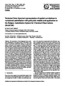
FIG. 1: The geometrical configuration (a) corresponding to two neutrons in the xz plane. R and r indicate the c.o.m position and the relative distance of the two neutrons.

(4)

where  α  14 

y 2 √ 1 e 2 αz z Hnz (z αz )

−r/2 r/2

(5)


1/2 h n⊥ ! i1/2 ϕn⊥ |m| (r⊥ , α⊥ ) = απ⊥ (n⊥ +|m|)!
2 √
|m| |m| 1 2 Ln⊥ α⊥ r⊥ × e 2 α⊥ r⊥ r⊥ α⊥

x (6)

In the above equations, αz and α⊥ are the HO parameters in the z and perpendicular directions, which are related to the HO frequencies by αz = M ωz /~ and α⊥ = M ω⊥ /~, respectively with M the nucleon mass, and Hnz and Ln⊥ are Hermite and Laguerre polynomials, respectively. Using the expansion (2) it can be shown that the pairing tensor in coordinate representation can be written in the following form (the spin up is donoted by ”+” and the spin down by ”-”) X κ (r~1 +, r~2 −) = ℜ|m1 |ν1 (re1 ) ℜ|m1 |ν2 (re2 ) m1 ≥0 ν1 ν2  m +1/2 (7) eim1 (θ1 −θ2 ) κ em11 ν1 ,m1 ν2  m −1/2 + (1 − δm1 ,0 ) e−im1 (θ1 −θ2 ) κ em11 ν1 ,m1 ν2 X κ (r~1 +, r~2 +) = − m1 ≥0 ν1 ν2  eim1 θ1 −i(m1 +1)θ2 ℜ|m1 |ν1 (re1 ) ℜ|m1 +1|ν2 (re2 ) m +1/2

×e κm11 ν1 ,m1 +1ν2

 (8) ℜ|m1 |ν1 (re2 ) ℜ|m1 +1|ν2 (re1 )

In the above expressions we have introduced the pairing tensor in the HO basis e e eΩ κα1 α2 ≡ κ e m1 ν1 ,m2 ν2 = 2s2 h0|cm1 s1 ν1 c−m2 −s2 ν2 |0i =κ eα2 α1

z=0

R

and

−e−i(m1 +1)θ1 +im1 θ2

z

(3)

The quantum numbers m and s are the projection of the orbital and spin momenta on symmetry (z) axis; ν are the radial quantum numbers ν = (n⊥ , nz ). The function ℜ|m|ν (e r ) ≡ ℜ|m|ν (r⊥ , z) is given by ℜ|m|ν (r⊥ , z) = ϕnz (z, αz ) × ϕn⊥ m (r⊥ , α⊥ )

r/2 −r/2

FIG. 2: The geometrical configuration (b) corresponding to two neutrons in the xy plane. R and r indicate the c.o.m position and the relative distance of the two neutrons.

in Figs.1-3; they have the advantage of a simple separa~ = (r~1 + r~2 )/2 tion between the center of mass (c.o.m) R and the relative ~r = r~1 − r~2 coordinates.

For a finite range force, as the D1S Gogny force used here, the pairing tensor has non-zero values for the total spin S = 0 and S = 1. How these two channels are related to the pairing tensors (7)-(8) depends on the geometrical configuration. Thus it can be shown that for the configuration displayed in Fig.1 the following rela-

y −r/2 r/2 R

z

(9)

where Ω = m1 + s1 = m2 + s2 . In the present study we calculate the pairing tensor corresponding to three geometrical configurations shown

FIG. 3: The geometrical configuration (c) corresponding to two neutrons in the yz plane. R and r indicate the c.o.m position and the relative distance of the two neutrons.

3 tions are satisfied: [κ (r~1 s1 , r~2 s2 )]00 =

√ 2 κ (r~1 +, r~2 −)

[κ (r~1 s1 , r~2 s2 )]10 = 0

(10) (11)

[κ (r~1 s1 , r~2 s2 )]11 = [κ (r~1 s1 , r~2 s2 )]1−1 = κ (r~1 +, r~2 +) (12) where the notation [..]ij means that the pairing tensor is coupled to total spin S = i with the projection Sz = j. For the configuration shown in Fig.2 the pairing tensor κ (r~1 s1 , r~2 s2 ) is a complex quantity and we have the relations √ [κ (r~1 s1 , r~2 s2 )]00 = 2 Re (κ (r~1 +, r~2 −)) (13) √ [κ (r~1 s1 , r~2 s2 )]10 = i 2 Im (κ (r~1 +, r~2 −))

(14)

[κ (r~1 s1 , r~2 s2 )]11 = [κ (r~1 s1 , r~2 s2 )]1−1 = κ (r~1 +, r~2 +) (15) Finally, for the configuration (c) of Fig.3, we have √ (16) [κ (r~1 s1 , r~2 s2 )]00 = 2 Re (κ (r~1 +, r~2 −)) [κ (r~1 s1 , r~2 s2 )]10 = 0

(17)

[κ (r~1 s1 , r~2 s2 )]11 = κ (r~1 +, r~2 +)

(18)

[κ (r~1 s1 , r~2 s2 )]1−1 = κ (r~1 −, r~2 −) = κ∗ (r~1 +, r~2 +) (19) The results for the pairing tensor shown in this paper are obtained by solving the HFB equations in a HO basis with 13 major shells for deformed nuclei. We have checked that by increasing the dimension of the basis the spatial properties of the pairing tensor do not change significantly up to distances of about 10 fm in the nuclei studied here. This shows that a finite discrete 13 major shell HO basis correctly describes these nuclei in the domain of interest of this work, in particular that continuum coupling effects can be ignored. III. A.

RESULTS AND DISCUSSION

Local and non-local parts of the pairing tensor

We shall start by shortly discussing the local part of the neutron pairing tensor. To illustrate the effect of the deformation, in Fig.4 is displayed the neutron local part of the pairing tensor for 152 Sm calculated in the spherical configuration β = 0 and in the deformed ground state β = 0.312, where β is the usual dimensionless deformation parameter. The color scaling on the right side of

FIG. 4: (Color online) The local part of the pairing tensor for 152 Sm. The upper and lower panels correspond to the spherical configuration and the deformed ground state, respectively.

plots indicates the intensity of the local part of the pairing tensor. In the spherical state the spatial structure of the local part of the pairing tensor can be simply traced back to the spatial localisation of a few orbitals with energies close to the chemical potential [7]. For 152 Sm the most important orbitals are 2f7/2 , 1h9/2 , 3p3/2 and 2f5/2 . As seen in Fig.4, in the deformed state the spatial pattern of the pairing tensor is more complicated. This stems from the fact that it requires quite many singleparticle configurations to explain its detailed structure. The spatial distribution of the configurations contributing the most to the pairing tensor are shown in Fig.5 ; the plots correspond to the contribution of single-particle states of given Ω and parity, with a different scaling for each panel. We shall focus now on the spatial structure of the nonlocal neutron pairing tensor. In Figs.6-8 are shown some

4

FIG. 5: (Color online) The spatial structure of the singleparticle blocks Ωπ which have the largest contribution to the pairing tensor shown in the bottom panel of Fig.4.

  ~ ~r |2 in the three geometrical contypical results of |κ R, figurations (a), (b) and (c) described in Fig.1-3 and for 152 Sm, 102 Sr and 238 U. At the spherical deformation, the 102 three geometrical configurations are equivalent.   For Sr 2 ~ ~r | is shown that manifests coexistence feature, |κ R,

only for the prolate minimum. For 238 U, the ground state as well as the isomeric state are displayed. The color scaling on the right side of plots indicates the intensity of the pairing tensor squared multiplied by a factor 104 . First of all we notice that the pairing tensor for S = 1 (Fig.6, bottom panel) is much weaker than for S = 0 (Fig.7, top panel) by a factor ∼ 20. This is a general feature in open shell nuclei (the pairing channel S=1 is significant in halo nuclei such as 11 Li). Therefore, in what follows we shall discuss only the channel S = 0. Figs.6-8 show that with deformation the pairing tensor is essentially confined along the direction of the c.o.mall coordinate. As in spherical nuclei, the pairing tensor can

~ ~r)2 for the isotope FIG. 6: (Color online) Non local κ(R, 152 Sm. The deformation is indicated by β and S is the spin. ~ ~r) is averaged over For the spherical case (upper panel), κ(R, ~ and ~r. For the deformed case (lower panel), the angles of R geometrical configuration (a) of Fig.1 has been adopted.

be preferentially concentrated either in the surface or in the bulk, depending on the underlying shell structure. The most interesting fact seen in Figs. 6-8 is the small spreading of pairing tensor in the relative coordinate. This is a feature we have already observed in spherical nuclei. In Ref.[3], it is discussed that the predilection for small spreading in the relative coordinate is caused by parity mixing. We will go back to this point in section III B. Quantitatively the spreading of the pairing tensor in the relative coordinate can be measured by the local coherence length (CL) defined in Ref.[8]. In the present study of deformed nuclei, as particular angular dependences are assumed according to the three geometrical configurations (a), (b) and (c), the following formula has

5

~ ~r)2 for the isotope FIG. 7: (Color online) Non local κ(R, 152 Sm. The deformation is indicated by β and S is the spin. (a), (b) and (c) indicate the geometrical configurations shown in Figs 1-3.

~ ~r)2 for isotopes 102 Sr FIG. 8: (Color online) Non local κ(R, 238 and U. For the latter are shown two cases corresponding to the ground state (middle panel) and to the fission isomer (bottom panel). Calculations have been made assuming configuration (a) of Fig.1.

6 been used: 12

(20)

The pairing tensor κ(R, r) corresponds to a given total spin S= 0 and a given geometrical configuration. For spherical nuclear configurations, the expression adopted for the CL is the standard one defined in Ref.[3] where ~ and ~r. averages are taken over both the angles of R In Fig.9, we present the neutron CL calculated for various deformed nuclei and configurations (a), (b) and (c) described in Fig.1-3. We notice that inside the nucleus the CL has large values, up to about 10-14 fm. This order of magnitude was already found in spherical nuclei. However, the CL displays much stronger oscillations compared to spherical nuclei, especially for the geometrical configurations (a) and (b). This behaviour can be attributed to the large number of different orbitals implied in pairing properties for deformed nuclei. An interesting feature seen in Fig.9 is the pronounced minimum of about 2 fm far out in the surface which appears for all isotopes and all geometrical configurations. The minimum found here has a similar magnitude as in spherical nuclei. A small coherence length of ∼ 2 fm in the surface of nuclei we have also found for the protons. In the proton case, the Coulomb force has not been taken into account in the pairing interaction but it is not expected to change the CL strongly.

(a)

10

(fm)

r4 |κ(R, r)|2 dr R r2 |κ(R, r)|2 dr

8 6 4 2 0 1 2 3 4 5 6 7 8 9 10

R(fm) 12

(b)

10

(fm)

ξ(R) =

sR

238

U Sm 102 Sr 102 Sr 152

8

=0.283 =0.312 =0.442 =-0.232

6 4 2

B.

0 1 2 3 4 5 6 7 8 9 10

Discussion of the coherence length

R(fm)

~ and where averages are taken over both the angles of R ~r. A possibility explaining the small CL in the surface of finite nuclei could be, as, e.g., suggested in [3], that pairing correlations are particularly strong there. Indeed, in the surface the neutron Cooper pairs have approximatively the same size as the deuteron, a bound pair. This is a situation similar to the strong coupling regime of pairing correlations. However, it is generally believed

14

(c)

12 10

(fm)

Compared to the smallest values of the CL in nuclear matter, of about 4-5 fm (see Fig.10 for symmetric and neutronic matter), the minimal values (∼ 2 fm) of the CL in nuclei are astonishingly small. The question which then arises is what causes such small values of the CL in the surface of nuclei. Since, as we have just mentioned, the general behaviour of the CL is similar in spherical and deformed nuclei, in what follows we shall focus the discussion on spherical nuclei. As a benchmark case, we will consider the isotope 120 Sn. In this case, the CL will be calculated as in Ref.[3], v uR 2 3 u 2 ~ ~ = t Rr |κ(R, ~r)| d r ξ(R) (21) ~ ~r)|2 d3 r |κ(R,

8 6 4 2 0 1 2 3 4 5 6 7 8 9 10

R(fm) FIG. 9: Coherence length for various isotopes. β denotes the deformation while (a),(b),(c) are the geometrical configurations shown in Figs. 1-3.

7 0.0 40

120

2.0

Sn -0.2

D1S

(fm)

30

1.5

Symmetric Neutronic

-0.4 1.0

20

0.5

10

0 0.001

-0.6

0.0 0 0.01

0.1

/

-0.8

2

1.

4

6

-1.0 10

8

R(fm)

0

0.0 60

2.0 FIG. 10: Coherence length in symmetric and neutronic matter according to the density normalized to the saturation density and calculated with the D1S Gogny force.

-0.2

Ec (R) = −

Ec (MeV) av (MeV) -0.4 n (R) / n(R=0)

1.5 1.0

that nuclei are with respect to pairing in the weak coupling limit [9]. In what follows, we shall examine whether there exists a correspondence between the magnitude of the CL and an enhancement of pairing correlations in the nuclear surface. Even though a local view can only give an incomplete picture because of fluctuations, a quantity which can be used to explore the spatial distribution of pairing correlations is the local pairing energy Z

Ni

-0.6

0.5 0.0 0

-0.8

2

4

6

-1.0 10

8

R(fm) 0.0

~ ~r)κ(R, ~ ~r), d3 r∆(R,

136

2.0

(22)

Sn -0.05

1.5

~ ~r) is the nonlocal pairing field. In practice where ∆(R, in Eq.(22), we use the angle-averaged quantities. The localisation properties of Ec (R) can be seen in Fig.11 (black line) where we show the results for several spherical nuclei. We notice that in the surface region where the minimum of the CL is located there is a local maximum of |Ec (R)| present for all nuclei considered. The largest value of Ec (R) (in absolute value) is not necessarily located in the surface region and the oscillations of the inner part of the distributions seem mostly due to shell fluctuations. In order to better exhibit a surface enhancement of pairing correlations, we have to consider a normalized pairing energy, otherwise the strong fall off of the density will mask to a great deal the local increase of pairing. One could divide Ec (R) by the local density, as done in [1]. However, here we prefer to divide by the local pairing density κ(R) = κ(R, 0), leading to the following definition of an average local pairing field Z 1 ~ ~r)κ(R, ~ ~r) ∆av (R) = d3 r∆(R, (23) κ(R)

-0.1

1.0

-0.15

0.5 0.0 0

2

4

6

-0.2 10

8

R(fm) 0.0 2.0

212

Pb -0.05

1.5 -0.1

1.0

-0.15

0.5 0.0 0

2

4

6

8

-0.2 10

R(fm) FIG. 11:

(Color online) Pairing correlation energies (right

8

In order to understand if this local enhancement of pairing correlations is able to explain the minimum value of ∼ 2 fm of the CL in the surface of finite nuclei, we have calculated the CL under the same conditions as before but with a variable factor α in front of the (S=0, T=1) pairing intensity of the D1S Gogny force (and only there). The result is shown in Fig.12 for α between 1.0 and 0.5 (top panel) for 120 Sn. It should be mentioned that for α = 1.0, the 120 Sn pairing energy is equal to ∼ 19MeV whereas for α = 0.5 it is ∼ 0.5MeV which can be considered as a very weak pairing regime. In spite of these extreme variations of the pairing field, the values of the CL are changing overall very little, except for R ≤ 1 fm. At R ≃ 6 fm, the variation is less than 0.2 fm. As we will see, this behavior is completely different in nuclear matter. From this study, it becomes clear that the CL is practically independent of the pairing intensity, in particular in the surface of finite nuclei. Therefore, we must revisit the interpretation proposed in our preceding paper [3], that the minimal size of ∼ 2 fm of Cooper pairs in the nuclear surface is a consequence of particularly strong local pairing correlations. From the fact that a completely different behavior is obtained in infinite nuclear matter (see below and Fig.16), the small size of the CL in the surface of nuclei seems to be strongly related to the finite size of the nucleus. At this stage of our analysis, it is important to clar-

12 120

10

(fm)

Sn =1.0 =0.9 =0.8 =0.7 =0.6 =0.5

8 6 4 2 0

2

4

6

8

10

R(fm)

12

120

Sn

10 Even Odd

8 (fm)

In practice in Eq.(23) we again use the angle-averaged quantities. We remark that with a zero range pairing force the above definition of the average pairing field gives the local pairing field. The localisation properties of ∆av (R) can be seen in Fig.11 (red line). We notice a qualitatively similar behavior as for Ec (R). However, due to the normalization, the average pairing field has significant values out in the surface region. A closer inspection of Fig.11 shows that the averaged pairing field reaches by 20% further out into the surface of the nucleus compared to the particle density (blue line). This can be quantified by the corresponding root mean squared values. This push of pairing correlations to the external region is determined by the localization properties of orbitals from the valence shell, which give the main contribution to the pairing tensor and pairing field. Since these states are less bound they are more spatially extended than the majority of states which determine the particle density and the nuclear radius. Moreover, the increase of the effective mass in the surface also probably plays an important role. Like the local pairing energy Ec (R), the average pairing field ∆av (R) presents a generic local maximum in the surface region with a local enhancement of pairing correlations (at tenth the matter density in 120 Sn, the average pairing field still reaches a relatively large value of ∼ 0.5MeV). On the other side, this maximum is not necessarily an absolute one and higher pairing field values can appear in the interior of nuclei, depending on the underlying shell structure.

6 4 2 0

2

4

6

8

10

R(fm) FIG. 12: (Color online) Coherence length calculated with total pairing tensor κ (top panel), even κe and odd κo part of the total pairing tensor (bottom panel) for different intensity of pairing strength, in the case of 120 Sn.

ify the role of parity mixing which was put forward in our preceding work [3] on the behaviour of the CL. In the bottom panel of Fig.12, is displayed the CL calculated either with the even part of the pairing tensor κe or with the odd one κo , for the same values of α as before. One sees that, in both cases, the value of the CL does not depend much on the intensity of the pairing. This conclusion holds here for all the values of R. Comparing the curves in the two panels of Fig.12, one sees that the even/odd CL’s have sensibly larger values in the center of the nucleus (around ∼ 10 fm) than the CL calculated with the full κ (6-8 fm), almost independently of the value of α. In the surface region they are practically of the same magnitude (2-3 fm). These results indicate that the parity mixing discussed in Ref. [3] influences the CL essentially for small values of R. Therefore, parity mixing cannot be the main reason for the small value

9 strength decreases, the height of the peak at r = 10 fm increases. In contrast, for R = 3, 6, 9 fm the influence of the parity mixing is very modest and the behaviour of X(R, r) is determined essentially by κ2e and κ2o . From R ≃ 3 fm to R ≃ 6 fm, one observes a sensitive reduction of the magnitude of X(R, r) leading to a lowering of the CL. In the vicinity of the surface (R ≥ 6 fm), the oscillatory behaviour of X(R, r) disappears. Here, single particle wave functions have almost reached their exponential regime. This explains why at R ≥ 6 fm, X(R, r) is characterized by only one major peak. The width of this major peak is minimum at the nuclear surface. Its broadening for R = 9 fm explains the increase of the CL beyond the nuclear surface.

FIG. 13: (Color online) Non-local part of the pairing tensor κ2 , even κ2e and odd κ2o part of the non-local part of the pairing tensor and the interference term 2κe κo for 120 Sn.

of the CL in the surface region. The trends observed in Fig.12 can be traced back to the variations of κ2 as well as κ2e , κ2o and the interference term 2κe κo plotted in Fig.13. One sees that the interference term is large only along the axes r = 0 and R = 0. However, in calculating the CL, |κ|2 is multiplied by a factor r4 in the numerator of Eq.(21). Hence, the large values of this interference term near r = 0 axis will not come into play significantly. Therefore, as observed previously, parity mixing will be significant essentially for R . 1 fm. This observation is confirmed by looking at the quantity X(R, r) =

r4 |κ (R, r) |2 N (R)

(24)

R∞ where N (R) = 0 dr r2 κ(R, r)2 . This quantity, once integrated over rR yields the square of the CL, Eq.(21) ∞ namely, ξ 2 (R) = 0 X(R, r)dr. X(R, r) is presented in Fig.14 for four values of R namely, 0, 3, 6 and 9 fm corresponding to the interior of the nucleus and the vicinity of the surface. The results are displayed for various values of the pairing factor α. Except for R = 0, X(R, r) and hence ξ(R) is not really sensitive to the strength of the pairing interaction. The large dependence of X(R, r) on the pairing strength at R = 0 comes from the comparatively large parity mixing already mentioned in connection with Fig.13, which is negative and maximum in absolute value for r ≃ 10 fm. Since the parity mixing tends to disappear as the pairing

A more global way to analyze the behavior of the CL is to consider directly the dependence on R of the numerator and the denominator of Eq.(21). This is shown in Fig.15. One sees, that independently of the value of α (the color code is the same as for Fig.12), the denominator decreases faster than the numerator around R = 6 fm and beyond. This sudden change in the slope of the denominator is accountable for the minimum value of CL. A similar analysis of the CL and of the influence of pairing correlations has been carried out in infinite matter. In Fig.16, we show the CL in infinite symmetric nuclear matter as a function of the density ρ normalized to its saturation value ρ0 , for the same α values as in the HFB calculations for finite nuclei. In the nuclear matter case, we see that the CL depends very strongly on the pairing intensity, whatever the density. For instance, the minimum value of CL increases a lot as pairing decreases. This behavior can be understood from an approximate analytic evaluation of the CL in infinite nuclear matter based on the definition Eq.(21) which differs only slightly from the usual Pippard expression [10] (see Appendix A):  
a2 2 3 1+ 3b − 12b + 4 + O(a ) ξnm 8 (25) ′ ′ where a = |∆F |/|ǫF |, b = kF ∆F /∆F with ∆F and ∆F the pairing field and its derivative for the Fermi momentum kF . As discussed in Appendix A, the correction terms in Eq.(25) are very small. ~2 kF = √ 2 2m∗ |∆F |

We see that the CL in infinite matter varies approximatively inversely proportional to the gap at the Fermi surface. This behavior is at variance with the results in finite nuclei and particularly where the CL shows the minimum, see Fig.12. This clearly indicates that the behavior of the CL, in particular the small value obtained in the surface of finite nuclei, is strongly influenced by the structure of the orbitals and that pairing plays a secondary role. In order to examine this question in more detail, we show in Fig.17 the extension of completely uncorrelated pairs made of Hartree-Fock neutron single particle wave functions. We use a definition of the extension of the pair

10

4.0

0.5

120

Sn

120

Numerator

2.0

1.0

0.0 0

0.08

0.3

Numerator

0.06

Denominator

0.04

0.2

0.02

0.1 2

4

6

8

10 12 14

r(fm)

0.0 0

2

4

6

8

0.0 10

R(fm)

3.0

R=3fm 120

FIG. 15: Evolution of numerator and denominator of ξ(R) for various values of α, in the case of 120 Sn.

Sn

X(R,r)

2.0

size similar to the CL of Eq.(21) namely, R

1.0

0.0 0

2

4

6

8

10 12 14

r(fm)

0.6

R=6fm 120

Sn

0.4 X(R,r)

=1.0 =0.9 =0.8 =0.7 =0.6 =0.5

0.2

0.0 0

2

4

6

8

10 12 14

r(fm)

0.8

R=9fm 0.6 X(R,r)

Sn

0.4

Denominator

X(R,r)

3.0

R=0fm

0.4

0.2

0.0 0

2

4

6

8

10 12 14

r(fm) FIG. 14: (Color online) X(R, r) for R=0, 3, 6 and 9 fm in the case of 120 Sn.

1/2 ~ ~r)|2 d3 r r2 |Ai (R, ξorb (R) =  1/2 R ~ ~r)|2 d3 r |Ai (R,

(26)

~ ~r) is defined The uncorrelated pair wave function Ai (R, as X ~ ~r) = 1 (2ji + 1) Ai (R, Cnnαi li ji Cnnβi li ji 4π nα nβ 1/2 X √ √ (27) (2l + 1) unl (r/ 2)uN l ( 2R) × (−)l 2li nN l × Pl (cosθ)hnlN l; 0|nα li nβ li 0i where Cnnαi li ji is the component of the (ni li ji ) neutron single-particle orbital on the HO basis function (nα li ji ). This equation is the same as Eq. (3) of Ref. [3] with the matrix κnliαjinβ of the pairing tensor replaced with the product of the two C coefficients. Since ξorb (R) corresponds to two non-interacting neutrons put into the same orbit and coupled to (L=0, S=0), it contains only the correlations induced by the confinement of the single-particle wave functions. As Fig.17 shows, ξorb has a pattern rather similar to the global CL displayed in Figs. 9 and 12, except for the 3s1/2 orbital. Thus, provided this orbital is not strongly populated, a change in the relative contributions of the single-particle states in the pairing tensor,e.g., induced by varying the intensity of pairing correlations, will not cause significant modifications in the global CL. This result has also been found by Pastore [11]. From Fig.17 we see that (except for 3s1/2 ), ξorb (R) exhibits a minimum in the surface of the order of ≃ 3.5 fm. This is indeed small but still larger than the 2.3 fm found with Eq.(21) for α = 1 (or 2.5 fm for α = 0.5). The reduction by about 30 percent from

11

(fm)

20

10

1.0 0.9 0.8 0.7 0.6

0.001

orb.

sm

(fm)

30

0.01

/

0.1

1.0

13 12 11 10 9 8 7 6 5 4 3 0

3s1/2 2d3/2 2d5/2 1g7/2 1h11/2

1

2

3

FIG. 16: (Color online) Coherence length calculated with different intensity of pairing strength in symmetric nuclear matter.

3.5 fm to 2.3 fm of the minimum of the CL is very likely due to the fact that even for very small pairing some orbit mixing takes place (remember that the influence of pairing is compensated in the ratio of numerator and denominator and that the chemical potential becomes not necessarily locked to a definite level but may stay in-between the levels). The cross terms of the wave functions can be negative yielding a possible explanation of the effect. Let us also point out that the CL implying only the even part of the pairing tensor (or the odd one), see [3], is of the order of ∼ 2.7 fm for 120 Sn, see Fig.12. Therefore, there should exist a slight influence of parity mixing in the CL calculated with the full κ. Nonetheless, the above discussion clearly indicates that the small value of the CL in the surface of finite nuclei is essentially due to the structure of the single particle wave functions. Our conclusion is somewhat different from the one put forward in our early paper [3]. There, we had not explored the behavior of the CL as a function of the pairing strength, which led us to conclude that the small size of Cooper pairs stems from a local strong coupling pairing regime. However, the other results and conclusions of Ref. [3] still hold. One may speculate about the reason for this radically different behavior of the CL in nuclei and infinite nuclear matter. One issue which certainly can be invoked, is that in macroscopic systems the number of single particle states in an energy range of the order of the gap is huge whereas in nuclei we only have a few states/MeV. In order to examine more precisely such an effect, let us consider, for convenience, the example of a spherical harmonic oscillator potential. We want to keep the essential finite size effects but eliminate unessential shell effects. It is well known that this can be achieved via the so-called Strutinsky smoothing. Single shells are washed

4

5

6

7

8

R(fm)

0

FIG. 17: Coherence length for Hartree-Fock single particle orbitals of the neutron valence shell of 120 Sn.

out and what remains is a continuum model with energy as variable, instead of individual discrete quantum states. We therefore can write for the pairing tensor in Wigner space: ~ ~p) = κ(R,

Z

~ p~) dEκ(E)f (E; R,

(28)

E

where κ(E) = uE vE is the Strutinsky averaged pair~ p~) is the Strutinsky averaged ing tensor [12] and f (E; R, Wigner transform of the density matrix on the energy shell E [13]. Integration of this quantity over energy up to the Fermi level yields the Strutinsky averaged density matrix in Wigner space. The latter quantity is shown in Fig. 1 of Ref. [14]. A particularity of the Strutinsky smoothed spherical ~ harmonic oscillator is that all quantities depend on R ~ and p~ only via the classical Hamiltonian Hcl. (R, ~p). We see that the Wigner transform of the density matrix is approximately constant for energies below the Fermi energy and drops to zero within a width of order ~ω. The corresponding density matrix on the energy shell can then be obtained from the quantity shown in Ref. [14] by differentiation with respect to energy. We, therefore, deduce that f (E; Hcl. ) is peaked around E ∼ Hcl. with a width of order ~ω. ~ p~) is, therefore, a The above integral over E in κ(R, convolution of two functions, one of width ∼ ∆ and the other one of width ∼ ~ω. As long as the gap is smaller ~ and ~p behavior of κ will be dominated than ~ω, the R by f (E; Hcl. ), i.e. by the oscillator wave functions. This is what happens in finite nuclei. On the contrary, in ~ ~p) is a infinite matter or in LDA descriptions, f (E; R, ~ δ-function, δ(E − Hcl. ), and then the R, p~ behavior of ~ ~p) is entirely determined by the width of κ(E), i.e. κ(R,

12 by the intensity of pairing. This interpretation qualitatively explains the very different behaviors of the CL with respect to the magnitude of pairing in finite nuclei and infinite matter. It also explains why the value of the CL in the surface of finite nuclei can be much smaller than the one calculated in infinite nuclear matter at any density. More quantitative investigations along this line are in preparation [15].

IV.

CONCLUSIONS

In this paper we have continued our study of the spatial properties of pairing correlations in finite nuclei. We first generalized our previous work [3] to deformed nuclei and found that the spatial behaviour of pairing is rather similar to the spherical case. This concerns, for instance, the remarkably small value of the coherence length (CL) (≃ 2 fm) in the nuclear surface. More inside the nucleus, sometimes more pronounced differences appear. We then concentrated on the reason for this strong minimal extension of the CL in the surface of nuclei. It was found that this feature is practically independent of the intensity of pairing and even seems to survive in the limit of very small pairing correlations. A detailed analysis of the quantities entering the definition of the CL indicates that, in finite nuclei, the latter is mainly determined by the single particle wave functions, i.e. by finite size effects. This eliminates suggestions that the strong observed lowering of the CL in the nuclear surface has something to do with especially strong pairing correlations in the surface [3], or in a surface layer, i.e. with a 2D effect [16]. A particular situation seems to prevail in the two neutron halo state of 11 Li [17]. We also made the same study in infinite nuclear matter. We found that in that case the CL strongly depends on the gap and an approximate inverse proportionality between the gap and the CL could be established. Concerning the reason why nuclei and infinite matter behave so differently with respect to the CL, we put forward the fact that the number of levels in the range of the gap value is huge in a macroscopic system whereas there are only a handfull of levels in finite nuclei. In such situations the numerator and denominator in the definition of the coherence length have a similar dependence on pairing and its influence tends to cancel. From this work, it appears that the CL may not be a good indicator of the spatial structure of pairing correlations in the case of nuclei or of other finite systems with a weak coupling situation like certain superconducting ultra small metallic grains [18]. This fact should not make us forget that on other quantities pairing in nuclei can have, as well known, a strong effect. For example the pairing tensor itself, as studied in this work, is very sensitive to parity mixing, see Fig.13, where a strong redistribution, i.e. a concentration of pairing strength along the c.o.m positions of the pairs takes place. Such a feature probably is

responsible for the strong enhancement of pair transfer into superfluid nuclei [19]. This small extension of the pairing tensor in the relative coordinate may not only be present in the surface but also in the bulk, depending somewhat on the shell structure. However, on average a generic but moderate enhancement of pairing correlations (obtained with the D1S Gogny force) is present in the nuclear surface, see Fig.11. Further elaboration of these aspects will be given in a forthcoming paper [15]. Acknowledgement We thank A. Pastore for sending us clarifying informations and for fruitfull discussions. We acknowledge also K. Hagino, Y. Kanada-Enyo, M. Matsuo, A. Machiavelli, H. Sagawa and X. Vi˜ nas for useful discussions. This work was partially supported by CNCSIS through the grant IDEI nr. 270. Appendix A: Neutron coherence length in infinite nuclear matter

Introducing the Wigner transform Z ~ ~k) = d3 r κ(R, ~ ~r)ei~k~r κW (R,

(A1)

~ ~r), the coherence of the HFB neutron pairing tensor κ(R, length (CL) defined by Eq. (21) can be rewritten v uR → ~ ~k)|2 u d3 k|− ∇ k κW (R, ~ ξ(R) = t R (A2) 3 ~ ~k)|2 d k|κW (R,

~ deIn infinite nuclear matter, κW is independent of R, ~ ~ pends on k only through the length k = |k|, and is given by κW (k) = ∆(k)/2E(k), where p ∆(k) is the HFB neutron pairing field and E(k) = (e(k) − µ)2 + ∆(k)2 the neutron quasiparticle energies with e(k) the singleneutron energies and µ the neutron chemical potential. Substituting these expressions into (A2) yields ξnm = p N/D with

Z ∞ 2 (e(k) − µ)2 (∆′ (k)(e(k) − µ) − ∆(k)e′ (k)) N= k 2 dk 3 [(e(k) − µ)2 + ∆(k)2 ] Z0 ∞ 2 ∆(k) D= k 2 dk (e(k) − µ)2 + ∆(k)2 0 (A3) The primed quantities are first derivatives. In order to be able to express the integrals analytically, we introduce the three following approximations 1. µ ≃ e(kF ) ≡ eF where kF is the neutron Fermi momentum, 2. e(k) ≃ ~2 k 2 /(2m∗ ) where m∗ is the kF -dependent neutron effective mass, 3. in the usual situation of nuclear physics where the gap values are much smaller than the Fermi energy,

13 the functions under the two integrals (A3) are sufficiently peaked around k = kF so that one can take ∆(k) ≃ ∆(kF ) ≡ ∆F and ∆′ (k) ≃ ∆′ (kF ) ≡ ∆′F .

Usually, a is much smaller than one, even at small densities. Expanding the above expressions around a = 0, one obtains

Using these assumptions and making the change of variables k = xkF , expressions (A3) become 2

N=a kF D=

a2 kF3

Z

∞

Z0

0

∞

 2 x2 (x2 − 1)2 b(x2 − 1) − 2x [(x2 − 1)2 + a2 ]3 x2 dx (x2 − 1)2 + a2

ξnm ∼ dx

1 √

akF

  a2 1 + (3b2 − 12b + 4) + O(a3 ) (A7) 8 2

(A4)

with a = |∆F /eF |, b = kf ∆′F /∆F . Assuming a 6= 0, the integrals on the right hand sides of (A4) can be calculated analytically using contour integration in the complex plane and the method of residues (more precisely, the integrand for N can be broken into an even function for which the integration range, as the one for D, can be extended from −∞ to +∞ and integrated by the method of residues, and an odd function which is easily integrated after the change of variable y = x2 ). One gets:   s  s √ √ 2 2 1 + 1 + a −1 + 1 + a  N=a2 kF 2π aY −X 2 2  # b 3π a −1 − + 3 cot (a) − 4a 2 1 + a2 s √ π 3 1 + 1 + a2 D= akF 2 2 (A5) where X and Y are functions of a and b given by a2 b2 (4a2 + 5) − 2(1 + a2 )(5a2 + 2) 64 a2 (1 + a2 )2 2 2 4 a b (21a + 35a2 + 12) + 4(1 + a2 )(7a2 + 4) Y = 128 a4 (1 + a2 )2 (A6) X=

[1] M.A. Tischler, A. Tonina, G.G. Dussel, Phys. Rev. C58 (1998) 2591. [2] M. Matsuo, K. Mizuyama, Y. Serizawa, Phys. Rev. C71 (2005) 064326. [3] N. Pillet, N. Sandulescu, P. Schuck, Phys. Rev. C76 (2007) 024310. [4] A. Pastore, F. Barranco, R. A. Broglia, E. Vigezzi, Phys. Rev. C78, (2008) 024315. [5] S. S. Pankratov, E. E. Saperstein, M. V. Zverev, M. Baldo, U. Lombardo, Phys. Rev. C79 (2009) 024309. [6] J. Decharg´e and D. Gogny, Phys. Rev. C21, (1980) 1568; J.-F. Berger, M. Girod, D. Gogny, Comp. Phys. Comm. 63 (1991) 365. [7] N. Sandulescu, P. Schuck, X. Vinas, Phys. Rev. C71 (2005) 054303. [8] F. V. De Blasio, M. Hjorth-Jensen, O. Elgaroy, L. En-

With a = |∆F |/(~2 kF2 /2m∗ ), the leading term yields 1 ~2 kF ξnm ∼ √ 2 2 m∗ |∆F |

(A8)

This expression is very close to the Pippard approximation of the CL [10]

ξP ippard =

1 ~2 kF π m∗ |∆F |

(A9)

√ the pre-factor being 1/2 2 ∼ 1/2.8 instead of 1/π. Usual values of a and b show that the first correction term in (A7) is very small. For instance, in symmetric nuclear matter at one tenth the normal density, one gets kF ≃ 0.6 fm−1 , a ≃ .2 and b ≃ .3 with the Gogny effective force, which yields 3.10−3 for this term. The next terms can be shown to be even smaller. Moreover, numerical evaluations of the integrands in (A3) for the Gogny force show that the three above approximations employed for deriving (A5), in particular the third one, are extremely well justified for densities ranging from zero to twice the normal density in symmetric nuclear matter.

[9] [10] [11] [12] [13] [14] [15] [16]

gvik, G. Lazzari, M. Baldo, H.-J. Schulze, Phys. Rev. C56 (1997) 2332. A. Bohr and B. Mottelson, Nuclear Structure, Vol. II, p.398. A.L. Fetter and J.D. Walecka, Quantum Theory of Manyparticle Systems, McGraw-Ill, New York, 1971. A. Pastore, PhD thesis, Milano, 2008; A. Pastore, private communications. M. Brack, P. Quentin, Nucl. Phys. A361(1981) 35 X. Vi˜ nas, P. Schuck, M. Farine, M. Centelles, Phys. Rev. C67(2003)054307. M. Prakash, S. Shlomo, V.M. Kolomietz, Nucl. Phys. A370 (1981) 30. X. Vi˜ nas, P. Schuck, N. Pillet, arXiv:1002.1459 [nucl-th]. Y. Kanada-Enyo, N. Hinohara, T. Suhara, P. Schuck, PRC 79(2009) 054305.

14 [17] K. Hagino, H. Sagawa, J. Carbonell, P. Schuck, Phys. Rev. Lett. 99 (2007) 022506 and arXiv:0912.4792 [nuclth].

[18] J. von Delft, D. C. Ralph, Phys. Rep., 345 (2001) 61. [19] W. von Oertzen, A. Vitturi, Rep. Prog. Phys. 64 (2001) 1247.