Type-2 Fuzzy Set Overview in Computational Intelligence Magazine

IE E Pr E oo f

IE E Pr E oo f

This article, "Type-2 Fuzzy Sets and Systems: An Overview," by Prof. Jerry M. Mendel (IEEE Computational Intelligence Magazine, vol. 2, no. 1, pp. 20-29, February 2007) presents an excellent overview of type-2 fuzzy sets and systems. As originally published in the February 2007 issue of IEEE Computational Intelligence Magazine, the article contained errors in mathematics that were introduced by the publisher. This

IE E Pr E oo f

corrected version is reprinted in its entirety.The IEEE regrets this error and extends its deepest apologies.We are deeply indebted to the author who has presented such a comprehensive survey.

IE E Pr E oo f

Jerry M. Mendel

IE E Pr E oo f

University of Southern California, USA

20

IEEE COMPUTATIONAL INTELLIGENCE MAGAZINE | FEBRUARY 2007

© 1994 DIGITALSTOCK CORP.

Abstract: This paper provides an introduction to and an overview of type-2 fuzzy sets (T2 FS) and systems. It does this by answering the following questions: What is a T2 FS and how is it different from a T1 FS? Is there new terminology for a T2 FS? Are there important representations of a T2 FS and, if so, why are they important? How and why are T2 FSs used in a rule-based system? What are the detailed computations for an interval T2 fuzzy logic system (IT2 FLS) and are they easy to understand? Is it possible to have an IT2 FLS without type reduction? How do we wrap this up and where can we go to learn more?

1556-603X/07/$25.00©2007IEEE

A T2 FS and How It is Different From a T1 FS

was recently asked “What’s the difference between the popular term fuzzy set (FS) and a type-1 fuzzy set (T1 FS)”? Before I answer this question, let’s recall that Zadeh introduced FSs in 1965 and type-2 fuzzy sets (T2 FSs) in 1975 [12]. So, after 1975, it became necessary to distinguish between pre-existing FSs and T2 FSs; hence, it became common to refer to the pre-existing FSs as “T1 FSs.” So, the answer to the question is “There are different kinds of FSs, and they need to be distinguished, e.g. T1 and T2.” I will do this throughout this overview article about T2 FSs and T2 fuzzy systems. Not only have T1 FSs been around since 1965, they have also been successfully used in many applications. However, such FSs have limited capabilities to directly handle data uncertainties, where handle means to model and minimize the effect of. That a T1 FS cannot do this sounds paradoxical because the word fuzzy has the connotation of uncertainty. This paradox has been known for a long time, but it is questionable who first referred to "fuzzy" being paradoxical, e.g. [3], p. [12]. Of course, uncertainty comes in many guises and is independent of the kind of FS or methodology one uses to handle it. Two important kinds of uncertainties are linguistic and random. The former is associated with words, and the fact that words can mean different things to different people, and the latter is associated with unpredictability. Probability theory is used to handle random uncertainty and FSs are used to handle linguistic uncertainty, and sometimes FSs can also be used to handle both kinds of uncertainty, because a fuzzy system may use noisy measurements or operate under random disturbances. Within probability theory, one begins with a probability density function (pdf) that embodies total information about random uncertainties. However, in most practical applications, it is impossible to know or determine the pdf; so, the fact that a pdf is completely characterized by all of its moments is used. For most pdfs, an infinite number of moments are required. Unfortunately, it is not possible, in practice, to determine an infinite number of moments; so, instead, enough moments are computed to extract as much information as possible from the data. At the very least, two moments are used—the mean and variance. To just use firstorder moments would not be very useful because random uncertainty requires an understanding of dispersion about the mean, and this information is provided by the variance. So, the accepted probabilistic modeling of random uncertainty focuses, to a large extent, on methods that use at least the first two moments of a pdf. This is, for example, why designs based on minimizing mean-squared errors are so popular. Just as variance provides a measure of dispersion about the mean, an FS also needs some measure of dispersion to capture more about linguistic uncertainties than just a single membership function (MF), which is all that is obtained when a T1 FS is used. A T2 FS provides this measure of dispersion.

What is a T2 FS and how is it different from a T1 FS? A T1 FS has a grade of membership that is crisp, whereas a T2 FS has grades of membership that are fuzzy, so it could be called a “fuzzy-fuzzy set.” Such a set is useful in circumstances where it is difficult to determine the exact MF for an FS, as in modeling a word by an FS. As an example [6], suppose the variable of interest is eye contact, denoted x, where x ∈[0, 10] and this is an intensity range in which 0 denotes no eye contact and 10 denotes maximum amount of eye contact. One of the terms that might characterize the amount of perceived eye contact (e.g., during an airport security check) is “some eye contact.” Suppose that 50 men and women are surveyed, and are asked to locate the ends of an interval for some eye contact on the scale 0–10. Surely, the same results will not be obtained from all of them because words mean different things to different people. One approach for using the 50 sets of two end points is to average the end-point data and to then use the average values to construct an interval associated with some eye contact. A triangular (other shapes could be used) MF, M F(x), could then be constructed, one whose base end points (on the x-axis) are at the two end-point average values and whose apex is midway between the two end points. This T1 triangular MF can be displayed in two dimensions, e.g. the dashed MF in Figure 1. Unfortunately, it has completely ignored the uncertainties associated with the two end points. A second approach is to make use of the average end-point values and the standard deviation of each end point to establish an uncertainty interval about each average end-point value. By doing this, we can think of the locations of the two end points along the x-axis as blurred. Triangles can then be located so that their base end points can be anywhere in the intervals along the x-axis associated with the blurred average end points. Doing this leads to a continuum of triangular MFs sitting on the x-axis, as in Figure1. For purposes of this discussion, suppose there are exactly N such triangles. Then at each value of x, there can be up to N MF values (grades), M F1 (x), M F2 (x), …, M FN (x) . Each of the possible MF grades has a weight assigned to it, say w x1 , w x2 , …, w xN (see the top insert in Figure 1). These weights can be thought of as the possibilities associated with each triangle’s grade at this value of x. Consequently, at each x, the collection of grades is a function {(M F i (x), w x i ), i = 1, …, N } (called secondary MF). The resulting T2 MF is 3-D. If all uncertainty disappears, then a T2 FS reduces to a T1 FS, as can be seen in Figure 1, e.g. if the uncertainties about the left- and right-end points disappear, then only the dashed triangle survives. This is similar to what happens in probability, when randomness degenerates to determinism, in which case the pdf collapses to a single point. In brief, a T1 FS is embedded in a T2 FS, just as determinism is embedded in randomness. It is not as easy to sketch 3-D figures of a T2 MF as it is to sketch 2-D figures of a T1 MF. Another way to visualize a T2 FS is to sketch (plot) its footprint of uncertainty (FOU) on

I

IE E Pr E oo f

Introduction

FEBRUARY 2007 | IEEE COMPUTATIONAL INTELLIGENCE MAGAZINE 21

IE E Pr E oo f

FIGURE 1 Triangular MFs when base end points (l and r) have uncertainty intervals associated with them. The top insert depicts the secondary MF (vertical slice) at x , and the lower insert depicts embedded T1 and T2 FSs, the latter called a wavy slice.

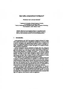
the 2-D domain of the T2 FS, and this is easy to do. The heights of a T2 MF (its secondary grades) sit atop its FOU. In Figure 1, if the continuum of triangular MFs is filled in (as implied by the shading), then the FOU is obtained. Another example of an FOU is shown in Figure 2. It is for a Gaussian primary MF whose standard deviation is known with perfect

certainty, but whose mean, m, is uncertain and varies anywhere in the interval from m1 to m2 . The uniform shading over the entire FOU means that uniform weighting (possibilities) is assumed. Because of the uniform weighting, this T2 FS is called an interval type-2 FS (IT2 FS). Almost all applications use IT2 FSs because, to date, it is only for such sets (and systems that use them) that all calculations are easy to perform. Additionally, although general T2 FSs have more design degrees of freedom (parameters) than IT2 FSs, no one knows yet how to best choose their secondary MFs. So, at this time there has been a logical progression from T1 to IT2. Although most applications use IT2 FSs, there is research underway about general T2 FSs and systems, e.g. [1] and [10]. New Terminology for a T2 FS

FIGURE 2 FOU for a Gaussian primary MF whose mean varies in the interval [m1 , m2 ] and whose standard deviation is a constant.

22

IEEE COMPUTATIONAL INTELLIGENCE MAGAZINE | FEBRUARY 2007

Is there new terminology for a T2 FS? Just as probability has much new terminology and definitions that must be learned in order to use it as a model of unpredictability, a T2 FS has new terminology and definitions that must be learned in order to use it as a model of linguistic uncertainty. New terms (some of which have already been used above) and definitions are summarized in Box 1. Note that in order to distinguish a T2 FS from a T1 FS, a tilde is used over the former, e.g. A˜ . Note, also, that an

BOX 1. New Terms for T2 FSs Term

Literal Definition (see Figure 1 for many of the examples)

Primary variable— x ∈ X Primary membership— J x

The main variable of interest, e.g. pressure, temperature, angle Each value of the primary variable x has a band (i.e., an interval) of MF values, e.g. J x  = [MF1 (x  ), MFN (x  )] An element of the primary membership, J x , e.g. u1 , . . . , uN The weight (possibility) assigned to each secondary variable, e.g. f x  (u1 ) = wx  1 A three-dimensional MF with point-value (x, u, µA˜ (x, u)), where x ∈ X, u ∈ J x , and 0 ≤ µA˜ (x, u) ≤ 1. Note that f x (u) ≡ µA˜ (x, u) A T1 FS at x, also called a vertical slice, e.g. top insert in Figure 1 ˜ the area between UMF (A) ˜ and The union of all primary memberships; the 2-D domain of A; ˜ LMF (A), e.g. lavender shaded regions in Figure 1 ˜ (see Figure 1) The lower bound of FOU(A) ˜ (see Figure 1) The upper bound of FOU(A)

Secondary variable— u ∈ J x Secondary grade— f x (u) Type-2 FS— A˜ Secondary MF at x Footprint of Uncertainty of ˜ A˜ − FOU(A) ˜ or µ (x) Lower MF of A˜ − LMF(A) A˜ ˜ ˜ or µ ˜ (x) Upper MF of A − UMF(A) A Interval T2 FS

IE E Pr E oo f

Embedded T1 FS— Ae (x) Embedded T2 FS— A˜e (x) Primary MF

A T2 FS whose secondary grades all equal 1, described completely by its FOU, e.g. Figure 3; ˜ where this notation means that the secondary grade equals 1 for all A˜ = 1/FOU(A) ˜ elements of FOU(A) Any T1 FS contained within A˜ that spans ∀x ∈ X; also, the domain for an embedded T2 FS, e.g. ˜ and UMF(A) ˜ the wavy curve in Figure 3, LMF(A) Begin with an embedded T1 FS and attach a secondary grade to each of its elements, e.g. see lower insert in Figure 1 Given a T1 FS with at least one parameter that has a range of values. A primary MF is any one of the T1 FSs whose parameters fall within the ranges of those variable parameters, e.g. the dashed MF in Figure 1

IT2 FS is completely characterized by its 2-D FOU that is bound by a lower MF (LMF) and an upper MF (UMF) (Figure 3), and, its embedded FSs are T1 FSs. Important Representations of a T2 FS

Are there important representations of a T2FS and, if so, why are they important? There are two very important representations for a T2 FS; they are summarized in Box 2. The vertical-slice representation is the basis for most computations, whereas the wavyslice representation is the basis for most theoretical derivations. The latter is also known as the Mendel-John Representation Theorem (RT) [8]. For an IT2 FS, both representations can also be interpreted as covering theorems because the union of all vertical slices and the union of all embedded T1 FSs cover the entire FOU.

FIGURE 3 Interval T2 FS and associated quantities.

BOX 2. Two Very Important Representations of a T2 FS Name of Representation Vertical-Slice Representation

Statement  Vertical slices (x) A˜ =

Comments Very useful for computation

∀x∈X

Wavy-Slice Representation

 A˜ = Embedded T2 FS ( j) ∀j

Very useful for theoretical derivations; also known as the Mendel-John Representation Theorem [8]

FEBRUARY 2007 | IEEE COMPUTATIONAL INTELLIGENCE MAGAZINE

23

FIGURE 4 Type-2 FLS.

Type-2 Fuzzy Logic Systems (FLS)

How and why are T2 FSs used in a rule-based system? A rulebased FLS [5, Ch. 1] contains four components—rules, fuzzifier, inference engine, and output processor—that are inter-connected, as shown in Figure 4. Once the rules have been established, a FLS can be viewed as a mapping from inputs to outputs (the solid path in Figure 4, from “Crisp inputs” to “Crisp outputs”), and this mapping can be expressed quantitatively as y = f (x). This kind of FLS is widely used in many engineering applications of fuzzy logic (FL), such as in FL controllers and signal processors, and is also known as a fuzzy controller or fuzzy system. Rules are the heart of an FLS. They may be provided by experts or extracted from numerical data. In either case, the rules can be expressed as a collection of IF–THEN statements, e.g. IF the total average input rate of real-time voice and video traffic is a moderate amount, and the total average input rate of the non-realtime data traffic is some, THEN the confidence of accepting the telephone call is a large amount. The IF-part of a rule is its antecedent, and the THEN-part of a rule is its consequent. FSs are associated with terms that appear in the antecedents or consequents of rules, and with the inputs to and output of the FLS. MFs are used to describe these FSs, and they can be

IE E Pr E oo f

Although the RT is extremely useful for theoretical developments, it is not yet useful for computation because the number of embedded sets in the union can be astronomical. Typically, the RT is used to arrive at the structure of a theoretical result (e.g., the union of two IT2 FSs), after which practical computational algorithms are found to compute the structure. For an IT2 FS, the RT states that an IT2 FS is the union of all of the embedded T1 FSs that cover its FOU. The importance of this result is that it lets us derive everything about IT2 FSs or systems using T1 FS mathematics [9]. This results in a tremendous savings in learning time for everyone.

BOX 3. How T1 FS Mathematics Can Be Used to Derive IT2 FS Fired-Rule Outputs [9]

In order to see the forest from the trees, focus on the single rule “IF x is F˜1 THEN y is G˜ 1 .” It has one antecedent and one consequent and is activated by a crisp number (i.e., singleton fuzzification). The key to using T1 FS mathematics to derive an IT2 FS fired-rule output is a graph like the one in Figure 5. Observe that the antecedent is decomposed into its nF T1 embedded FSs and the consequent

is decomposed into its nG T1 embedded FSs. Each of the nF × nG paths (e.g., the one in lavender) acts like a T1 inference. When the union is taken of all of the T1 firedrule sets, the result is the T2 firedrule set. The latter is lower and upper bound, because each of the T1 fired-rule sets is bound. How to actually obtain a formula for B(y) is explained very carefully in [9], and just requires computing these lower and upper bounds—and they only involve lower and upper MFs of the antecedent and consequent FOUs. How this kind of graph and its associated analyses are extended to rules that have more than one antecedent, more than one rule, and other kinds of fuzzificaFIGURE 5 Graph of T1 fired-rule sets for all possible nB = nF × nG combinations of embedded tions is also explained in [9]. T1 antecedent and consequent FSs, for a single antecedent rule.

24 IEEE COMPUTATIONAL INTELLIGENCE MAGAZINE | FEBRUARY 2007

Box 4. Pictorial Descriptions for T1 and T2 Inferences Figure 6 depicts input and antecedent operations for a two-antecedent single-consequent rule, singleton fuzzification, and minimum tnorm. When x1 = x1 , µF1 (x1 ) occurs at the intersection of the vertical line at x1 with µF1 (x1 ); and, when x2 = x2 , µF2 (x2 ) occurs at the intersection of the vertical line at x2 with µF2 (x2 ). The firing level is a number equal to min [µF1 (x1 ), µF2 (x2 )]. The main thing to observe from this figure is that the result of input and antecedent operations is a number—the firing level f (x ). This firing level is then t-normed with the entire consequent set, G. When µG (y) is a triangle and the t-norm is minimum, the resulting fired-rule FS is the trapezoid shown in red. Figure 7 shows the comparable calculations for an IT2 FLS. Now when x1 = x1 , the vertical line at x1 intersects FOU(F˜1 ) everywhere in the interval [µF˜ (x1 ), µ¯ F˜1 (x1 )]; and, when x2 = x2 , the vertical line at x2 intersects FOU(F˜2 ) everywhere in the interval 1 ¯  ), where [µF˜ (x2 ), µ¯ F˜2 (x2 )]. Two firing levels are then computed, a lower firing level, f(x ), and an upper firing level, f(x   2 ¯  ) = min[µ¯ ˜ (x  ), µ¯ ˜ (x  )]. The main thing to observe from this figure is that the result of input f(x ) = min[µF˜ (x1 ), µF˜ (x2 )] and f(x 1 2 F F 1 2 1 2 ¯  )]. f(x ) is then t-normed with LMF(G) ˜ and antecedent operations is an interval—the firing interval F(x ), where F(x ) = [f(x ), f(x  ¯ ˜ ˜ and f(x ) is t-normed with UMF(G). When FOU(G) is triangular, and the t-norm is minimum, the resulting fired-rule FOU is the yel-

IE E Pr E oo f

low trapezoidal FOU.

FIGURE 6 T1 FLS inference: from firing level to rule output.

x1

x1

FOU (B )

x2

x2

FIGURE 7 IT2 FLS inference: from firing interval to rule output FOU.

FEBRUARY 2007 | IEEE COMPUTATIONAL INTELLIGENCE MAGAZINE

25

BOX 5. A comparison of COS defuzzification and TR Center-of-Sets (COS) Defuzzification, ycos (x) 1. Compute the centroid of each rule's consequent T1 FS. Call it c l (l = 1, ..., M) 2. Compute the firing level for each (fired) rule. Call it f l (l = 1, ..., M)  M M   cl f l fl 3. Compute ycos (x) = l=1

l=1

Center-of-Sets (COS) TR, Ycos (x) l l 1. Compute the centroid of each rule's consequent IT2 FS,  using  the KM algorithms (see Box 6). Call it [yl , yr ] (l = 1, ..., M) l 2. Compute the firing interval for each (fired) rule. Call it f , f¯l (l = 1, ..., M) 3. Compute Ycos (x) = [yl (x), yr (x)], where yl (x) is the solution to the following minimization problem, yl (x) =    M M   min yll f l f l , that is solved using a KM Algorithm (Box 6), and yr (x) is the solution to the following maximization problem, l ∀f l ∈[f ,f¯l ] l=1  l=1   M M   yr (x) = max yrl f l f l , that is solved using the other KM Algorithm (Box 6). l=1

l=1

IE E Pr E oo f

l ∀f l ∈[f ,f¯l ]

BOX 6. Centroid of an IT2 FS and its computation

Consider the FOU shown in Figure 8. Using the RT, compute the centroids of all of its embedded T1 FSs, examples of which are shown as the colored functions. Because each of the centroids is a finite number, this set of calculations leads to a set of centroids ˜ C(B). ˜ C(B) ˜ has a smallest value c l that is called the centroid of B, ˜ ˜ So, to compute ˜ and a largest value cr , i.e. C(B) = [c l (B), cr (B)]. ˜ C(B) it is only necessary to compute c l and cr . It is not possible to

using two iterative algorithms that are called the Karnik-Mendel (KM) algorithms. ˜ Note that c l = min (centroid of all embedded T1 FSs in FOU(B)). Analysis shows that: L

c l = c l (L) =

i=1

L

˜ i )+ N ˜ yi UMF(B|y i=L+1 yi LMF(B|yi ) N ˜ ˜ UMF(B|yi ) + LMF(B|yi )

i=1

i=L+1

do this in closed form. Instead, it is possible to compute c l and cr

One of the KM algorithms computes switch point L (see Figure 9). Note also that cr = max (centroid of all embedded T1 FSs in ˜ Analysis shows that: FOU(B)). R

cr = cr (R) =

˜

i=1 yi LMF(B|yi ) + R ˜ i=1 LMF(B|yi ) +

N

i=R+1

N

i=R+1

˜ i) yi UMF(B|y ˜ i) UMF(B|y

The other KM algorithm computes switch point R (see Figure 10).

Derivations and statements of the KM algorithms are found, e.g., in [2, pp. 204–207] and [5, pp. 258–259 or pp. 308–311].

FIGURE 8 FOU and some embedded T1 FSs.

FIGURE 9 The red embedded T1 FS is used to compute c l (L).

26

IEEE COMPUTATIONAL INTELLIGENCE MAGAZINE | FEBRUARY 2007

FIGURE 10 The red embedded T1 FS is used to compute cr (R).

either T1 or T2. The latter lets us quantify different kinds of uncertainties that can occur in an FLS. Four ways in which uncertainty can occur in an FLS are: (1) the words that are used in antecedents and consequents of rules can mean different things to different people; (2) consequents obtained by polling a group of experts will often be different for the same rule, because the experts will not necessarily be in agreement; (3) only noisy training data are available for tuning (optimizing) the parameters of an IT2 FLS; and (4) noisy measurements activate the FLS. An FLS that is described completely in terms of T1 FSs is called a T1 FLS, whereas an FLS that is described using at least one T2 FS is called a T2 FLS. T1 FLSs are unable to directly handle these uncertainties because they use T1 FSs that are certain. T2 FLSs, on the other hand, are very useful in circumstances where it is difficult to determine an exact MF for an FS; hence, they can be used to handle these uncertainties.

Almost all applications use IT2 FSs because all calculations are easy to perform. Returning to the Figure 4 FLS, the fuzzifier maps crisp numbers into FSs. It is needed to activate rules that are in terms of linguistic variables, which have FSs associated with them. The inputs to the FLS prior to fuzzification may be certain (e.g., perfect measurements) or uncertain (e.g., noisy measurements). The MF for a T2 FS lets us handle either kind of measurement. The inference block of the Figure 4 FLS maps FSs into FSs. The most commonly used inferential procedures for a FLS use minimum and product implication models. The resulting T2 FLSs are then called Mamdani T2 FLSs. TSK T2 FLSs are also available [5].

BOX 7. Uncertainty Bounds and Related Computations

IE E Pr E oo f

1. Compute Centroids of M Consequent IT2 FSs yli and yri (i = 1, ..., M), the end points of the centroids of the M consequent IT2 FSs, are computed using the KM algorithms (Box 6). These computations can be performed after the design of the IT2 FLS has been completed and they only have to be done once. 2. Compute Four Boundary Type-1 FLS Centroids  M M i i f yli f yl(0) (x) = i=1

yl(M) (x) =

M

i=1

f¯i yli

M

f¯i yri

 M

i=1

 M

i=1

yr(()) (x) =

f¯i

yr(M) (x) =

i=1

M

f¯i

i=1

i

f yri

 M

i=1

f

i

i=1

3. Compute Four Uncertainty Bounds y (x) ≤ yl (x) ≤ y¯ l(x) l

y (x) ≤ yr (x) ≤ y¯ r (x) r

 y¯ l(x) = min yl(0) (x), yl(M) (x) 

 y (x) = max yr()) (x), yr(M) (x) r

M  i ¯i  (f − f )  i=1 y (x) = y¯ l(x) −  l M M    i f f¯i i=1

M  i ¯i  (f − f )  i=1 y¯ r (x) = y (x) +  r M M    i f f¯i

i=1

i=1

 M    f yli − yl1 f¯i ylM − yli   i=1 i=1 ×  M M    M   i i 1 i ¯ i f yl − yl f yl − yl + M 

i=1

i



i=1

 M M     i f yrM − yri  f¯i yri − yr1  i=1 i=1 ×  M M      i M ¯ i i 1 i f yr − yr + f yr − yr

i=1

i=1

i=1

Note: The pair y¯ t (x), yr (x) are called inner (uncertainty) bounds, whereas the pair yl (x), y¯ r (x) are called outer (uncertainty) bounds. 4. Compute Approximate TR Set [yl (x), yr (x)] ≈ [yˆ l(x), yˆ r (x)] = [(y (x) + y¯ l(x))/2, (y (x) + y¯ r (x))/2] l

r

5. ComputeApproximate Defuzzified Output ˆ y(x) ≈ y(x) = 12 [yˆ l(x) + yˆ r (x)]

FEBRUARY 2007 | IEEE COMPUTATIONAL INTELLIGENCE MAGAZINE

27

trol action. In a signal processing application, such a number could correspond to a financial forecast or the location of a target. The output processor for a T1 FLS is just a defuzzifier; however, the output processor of a T2 FLS contains two components: the first maps a T2 FS into a T1 FS and is called a type-reducer [that performs type-reduction (TR)], and the second performs defuzzification on the type-reduced set. To date, practical computations for a T2 FLS are only possible when all T2 FSs are IT2 FSs, i.e. for an IT2 FLS.

There are two very important representations for a T2 FS vertical-slice and wavy-slice representations. In many applications of an FLS, crisp numbers must be obtained at its output. This is accomplished by the output processor, and is known as defuzzification. In a control-system application, for example, such a number corresponds to a con-

Computations in an IT2 FLS Firing Level (FL) Type-Reduction (TR) −j Upper f (x) FL Input x Lower FL

f j (x) −

Up to M Fired Rules (j = 1,..., M)

yl (x)

Center-of Sets TR (Uses KM Consequent IT2 FS Centroids Algorithms) yj l Left End Associated Consequent

y(x)

Right End

y rj

AVG

yr (x)

with Fired Rules (j = 1,..., M)

Memory

FIGURE 11 Computations in an IT2 FLS that use center-of-sets TR.

Input x

Firing Level (FL) Uncertainty Bounds −j Upper f (x) FL yl Left − LB j Lower f− (x) FL

Left UB

y−l

Defuzzification

∧

yl (x)

AVG

∧

y (x)

AVG

Consequent IT2 FS Centroids

Consequent UMFs and LMFs

Left End

Right End

yj l

Right LB

yr −

∧

AVG

y rj

Right UB

yr (x)

y−r

Memory FIGURE 12 Computations in an IT2 FLS that use uncertainty bounds instead of TR. LB = lower bound, and UB = upper bound.

28

What are the detailed computations for an IT2 FLS and are they easy to understand? As mentioned above, the RT can be used to derive the input-output formulas for an IT2 FLS. How the formulas are derived from the (see Figure 4) input of the Inference block to its output is explained in Box 3. Because practitioners of T1 FLSs are familiar with a graphical interpretation of the inference engine computation, T1 computations are contrasted with T2 computations in Box 4. Comparing Figures. 6 and 7, it is easy to see how the uncertainties about the antecedents flow through the T2 calculations. The more (less) the uncertainties are, then the larger (smaller) the firing interval is and the larger (smaller) the fired-rule FOU is. Referring to Figure 4, observe that the output of the Inference block is processed next by the Output Processor that consists of two stages, Type-reduction (TR) and Defuzzification. All TR methods are T2 extensions of T1 defuzzification methods, each of which is based on some sort of centroid calculation. For example, in a T1 FLS, all fired-rule output sets can first be combined by a union operation after which the centroid of the resulting T1 FS can be computed. This is called centroid defuzzification. Alternatively, since the union operation is computationally costly, each firing level can be combined with the centroid of its consequent set, by means of a different centroid calculation, called center-of-sets defuzzification (see top portion of Box 5). The T2 analogs of these two kinds of defuzzification are called centroid TR and center-of-sets TR (see bottom portion of Box 5 and also [5] for three other kinds of TR). The result of TR for IT2 FSs is an interval set [y l (x), y r (x)].

IE E Pr E oo f

UMFs and LMFs

Defuzzification

IEEE COMPUTATIONAL INTELLIGENCE MAGAZINE | FEBRUARY 2007

Regardless of the kind of TR, they all require computing the centroid of an IT2 FS. Box 6 explains what this is and how the centroid is computed. The two iterative algorithms for doing this are known as the Karnik-Mendel (KM) algorithms [2], and they have the following properties: 1) they are very simple, 2) they converge to the exact solutions monotonically and super-exponentially fast, and 3) they can be run in parallel, since they are independent. Defuzzification, the last computation in the Figure 4 IT2 FLS, is performed by taking the average of y l (x) and y r (x). The entire chain of computations is summarized in Fig. 11. Firing intervals are computed for all rules, and they depend explicitly on the input x. For center-of-sets TR (see Box 5), off-line computations of the centroids are performed for each of the M consequent IT2 FSs using KM algorithms, and are then stored in memory. Center-of-sets TR combines the firing intervals and pre-computed consequent centroids and uses the KM algorithms to perform the actual calculations. An IT2 FLS for Real-Time Computations

tainties about words. It is anticipated that by using more general T2 FSs and FLSs it will be possible to capture higher-order uncertainties about words. Much remains to be done. For readers who want to learn more about IT2 FSs and FLSs, the easiest way to do this is to read [9]; for readers who want a very complete treatment about general and interval T2 FSs and FLSs, see [5]; and, for readers who may already be familiar with T2 FSs and want to know what has happened since the 2001 publication of [5], see [7].

IE E Pr E oo f

Is it possible to have an IT2 FLS without TR? TR is a bottleneck for real-time applications of an IT2 FLS because it uses the iterative KM algorithms for its computations. Even though the algorithms are very fast, there is a time delay associated with any iterative algorithm. The good news is that TR can be replaced by using minimax uncertainty bounds for both y l (x) and y r (x). These bounds are also known as the Wu-Mendel uncertainty bounds [11]. Four bounds are computed, namely lower and upper bounds for both y l (x) and y r (x). Formulas for these bounds are only dependent upon lower and upper firing levels for each rule and the centroid of each rule’s consequent set, and, because they are needed in two of the other articles in this issue, are given in Box 7. Figure 12 summarizes the computations in an IT2 FLS that uses uncertainty bounds. The front end of the calculations is identical to the front end using TR (see Figure 11). After the uncertainty bounds are computed, the actual values of y l (x ) and y r (x ) (that would have been computed using TR, as in Figure 11) are approximated by averaging their respective uncertainty bounds, the results being yˆ l (x ) and yˆ r (x ). Defuzzification is then achieved by averaging these two approximations, the result being yˆ (x), which is an approximation to y(x). Remarkably, very little accuracy is lost when the uncertainty bounds are used. This is proven in [11] and has been demonstrated in [4]. See [7] for additional discussions on IT2 FLSs without TR. In summary, IT2 FLSs are pretty simple to understand and they can be implemented in two ways, one that uses TR and one that uses uncertainty bounds.

FIGURE 13 Educational perspective of T2 FSs and FLSs.

Conclusions

How do we wrap this up and where can we go to learn more? In school, we learn about determinism before randomness. Learning about T1 FSs before T2 FSs fits a similar learning model (Figure 13). IT2 FSs and FLSs let us capture first-order uncer-

Acknowledgements

The author acknowledges the following people who read the draft of this article and made very useful suggestions on how to improve it: Simon Coupland, Sarah Greenfield, Hani Hagras, Feilong Liu, Robert I. John and Dongrui Wu. References

Note: This is a minimalist list of references. For many more references about T2 FSs and FLSs, see [5] and [7]. Additionally, the T2 Web site http://www.type2fuzzylogic.org/ is loaded with references and is being continually updated with new ones.

[1] S. Coupland and R.I. John, “Towards more efficient type-2 fuzzy logic systems,” Proc. IEEE FUZZ Conf., pp. 236–241, Reno, NV, May 2005. [2] N.N. Karnik and J.M. Mendel, “Centroid of a type-2 fuzzy set,” Information Sciences, vol. 132, pp. 195–220, 2001. [3] G.J. Klir and T.A. Folger, “Fuzzy Sets, Uncertainty, and Information,” Prentice Hall, Englewood Cliffs, NJ, 1988. [4] C. Lynch, H. Hagras and V. Callaghan, “Using uncertainty bounds in the design of an embedded real-time type-2 neuro-fuzzy speed controller for marine diesel engines,” Proc. IEEE-FUZZ 2006, pp. 7217–7224, Vancouver, CA, July 2006. [5] J.M. Mendel, “Uncertain Rule-Based Fuzzy Logic Systems: Introduction and New Directions,” Prentice-Hall, Upper-Saddle River, NJ, 2001. [6] J.M. Mendel, “Type-2 fuzzy sets: some questions and answers,” IEEE Connections, Newsletter of the IEEE Neural Networks Society, vol. 1, pp. 10–13, 2003. [7] J.M. Mendel, “Advances in type-2 fuzzy sets and systems,” Information Sciences, vol. 177, pp. 84–110, 2007. [8] J.M. Mendel and R.I. John, “Type-2 fuzzy sets made simple,” IEEE Trans. on Fuzzy Systems, vol. 10, pp. 117–127, April 2002. [9] J.M. Mendel, R.I. John, and F. Liu, “Interval type-2 fuzzy logic systems made simple,” IEEE Trans. on Fuzzy Systems, vol. 14, pp. 808–821, Dec. 2006. [10] J.T. Starczewski, “A triangular type-2 fuzzy logic system,” Proc. IEEE-FUZZ 2006, pp. 7231–7238, Vancouver, CA, July 2006. [11] H. Wu and J.M. Mendel, “Uncertainty bounds and their use in the design of interval type-2 fuzzy logic systems,” IEEE Trans. on Fuzzy Systems, vol. 10, pp. 622–639, Oct. 2002. [12] L.A. Zadeh, “The concept of a linguistic variable and its application to approximate reasoning–1,” Information Sciences, vol. 8, pp. 199–249, 1975.

FEBRUARY 2007 | IEEE COMPUTATIONAL INTELLIGENCE MAGAZINE

29

IE E Pr E oo f

IE E Pr E oo f