Birkhauser, Boston, 1997. [6] Dmitri Chiriaev and G. William Walster. ... [7] William D. Clinger. How to read floating ... [10] Charles Farnum. Compiler support for ...
Type System Support for Floating-Point Computation E. Jason Riedy For Cs279, Spring 2001 May 25, 2001 Abstract Floating-point arithmetic is often seen as untrustworthy. We show how manipulating precisions according to the following rules of thumb enhances the reliability of and removes surprises from calculations: • Store data narrowly, • compute intermediates widely, and • derive properties widely. Further, we describe a typing system for floating point that both supports and is supported by these rules. A single type is established for all intermediate computations. The type describes a precision at least as wide as all inputs to and results from the computation. Picking a single type provides benefits to users, compilers, and interpreters. The type system also extends cleanly to encompass intervals and higher precisions.
1
Introduction
Programmers are generally wary of floating-point arithmetic. Most consider it an unfortunate approximation. Programmers are generally advised never to trust floating-point computations unless they are very precise. Even then, most avoid ever testing numbers for equality, and almost all consider unexpected results a problem of the arithmetic. Why is that? The features in Ieee754 [13] were developed to ensure that programmers could create accurate, safe, and unsurprising code. Yet many of these features remain unavailable to programmers, trapped under levels of programming systems that consider them unimportant or even ill-conceived. Here we consider one aspect of how floating-point computations are exposed to programmers, through control of the precisions available. We find that higher precisions do not provide a solution on their own, but that combining precisions judiciously can reduce or even eliminate the need for recriminations against floating-point arithmetic. We should not simply throw higher precisions against
1
Type Single Double Extended∗ Quadruple
Significand width
ε −24
2 ≈ 6.0 × 10⁻⁸ −53 2 ≈ 1.1 × 10⁻¹⁶ −64 2 ≈ 1.1 × 10⁻¹⁹ −113 2 ≈ 9.6 × 10⁻³⁵
24 bits 53 bits 64 bits 113 bits
Table 1: Ieee754 floating-point precisions, where extended is the doubleextended type as implemented by Intel and Motorola problems but rather consider the interplay between wide and narrow precisions when choosing data types for reliable software. We maintain that the following rules of thumb help reduce the incidence of surprises [19]: • Store data in the narrowest representation reasonable, • compute intermediate results in the widest representation feasible, and • derive important properties in wider precisions. Each rule supports the others, although at first they appear contradictory. Assisting these rules in language systems requires an examination of evaluation disciplines. A language or its compiler must specify to which precision any given floating-point arithmetic expression is evaluated. There are only three sensible evaluation disciplines: strict, widest needed, and widest feasible. Strict evaluation is a local typing; every subexpression’s result is delivered in the widest precision of its immediate inputs. Widest need generalizes this to the entire expression. The widest input to a given expression determines the result type of all subexpressions. Evaluating to the widest feasible type finds the widest needed precision and then expands that if possible to the widest precision available that runs quickly. On many architectures, this corresponds to double precision. Intel architectures provide an extended scalar precision at the same speed, so there the widest feasible precision is no narrower than extended. Note that if not all variables are annotated with types, or if they are annotated with an expression type, expressions can span large amounts of the source code. Section 2 demonstrates how applying these rules of thumb helps make some simple calculations accurate. Then Section 3 describes type system support for these rules of thumb. We demonstrate that the widest feasible and widest needed disciplines not only make numeric sense, they also make traditional arithmetic typing problems simpler. Section 4 presents implementation considerations, including some subtleties and possible optimizations. Extending the type system to intervals and further precisions is covered in Section 5. Finally, Section 6 offers concluding remarks, and Section 7 points to problems that remain. The precisions used through most of the discussions are defined by Ieee 7541 and are given in Table 1. The ε term is half the distance from 1.0 to the next 1 I’m
taking for granted that quadruple precision will be included in the revision.
2
largest floating-point number in the same precision. Numerical errors in single are generally modeled as multiplicative perturbations by 1 + δ with |δ| ≤ ε [9].
2
Motivation
As in [27], examine what happens when we compute2 f (x) = sin2 x + cos2 x from single-precision inputs ranging from 0 to π/4 in steps of 2−20 . If all intermediate quantities are computed in single-precision, we find that 91 579 of the computed values are not equal to one! Computing everything and returning a result in double and quad precision produces 88 169 and 90 623 surprising values, respectively. Increasing the precision does not significantly improve the results. Now compute a single-precision result from f and a single-precision x evaluating all intermediate terms to double precision. How many values are not one? None. The same lack of surprise comes from quadruple precision. Computing with more precision than the data and output appeared to ‘deserve’ produced the result users should expect. Increasing precision does not remove the effects of finite precision, but higher precision can forestall their onset when used appropriately. Simple problems can then be handled simply.
2.1
Evaluate Widely and Examine Narrowly
Do narrow data deserve wider intermediates? Consider Figure 1. The graphs depict the polynomial p(x) = x3 − 45x2 + 675x − 3375
(1)
with single-precision coefficients and around 4 000 single-precision inputs x from 14.8 to 15.2. The coefficients can be converted to binary floating point exactly. Now p(x) = (x − 15)3 algebraically, so the interval spans a triple root. Evaluating expanded polynomials near roots involves a good deal of cancellation. The higher the root’s multiplicity, the wider the region of arguments where cancellation occurs. If the intermediate variables are too narrow, all the information that cancellation would reveal is lost. The cancellation is accused of being destructive, while the information was lost to a too-narrow precision. Figure 1(a) depicts this graphically. The polynomial is evaluated simply. Each term is individually evaluated in single precision by multiplying the coefficient with x repeatedly, then the term is added into a single-precision accumulator. Clearly, a great deal of information is lost. Imagine passing this evaluation to a root finding routine that finds roots by identifying sign changes. How many roots can this routine find? Such routines require tolerances to avoid finding huge numbers of roots, increasing the range of numbers treated as zero. What users would suspect a polynomial representable 2 On
a Sun UltraSparc iie running Solaris 8
3
0.01
0.01
0.008
0.008
0.006
0.006
0.004
0.004
0.002
0.002
0
0
-0.002
-0.002
-0.004
-0.004
-0.006
-0.006 -0.008
-0.008 -0.01 14.8
14.85
14.9
14.95
15
15.05
15.1
15.15
-0.01 14.8
15.2
(a) Simple evaluation in single precision
14.85
14.9
14.95
15
15.05
15.1
15.15
15.2
(b) Horner’s rule in single precision
0.008 0.006 0.004 0.002 0 -0.002 -0.004 -0.006 -0.008 14.8
14.85
14.9
14.95
15
15.05
15.1
15.15
15.2
(c) Simple evaluation in double precision
Figure 1: The polynomial x3 − 45x2 + 675x − 3375 = (x − 15)3 evaluated near its root, 15. The graphs show values from single-precision intermediates without and with Horner’s rule, and double-precision intermediates without Horner’s rule. exactly in single precision would require a tolerance around 2 × 10⁻³ when normalized single precision extends to almost 10−38 ? People with some training in computer science might remember a faster way to evaluate a polynomial, Horner’s rule. With Horner’s rule, we re-write the polynomial as p(x) = ((x − 45) ∗ x + 675) ∗ x − 3375. (2) Evaluation proceeds by evaluating the simple expressions into an accumulator from the inside out. Not only is it faster, it is also more stable in floating-point arithmetic. Figure 1(b) demonstrates the improved stability. An error analysis of both evaluation techniques gives error bounds that are fairly tight; the bounds match each plot’s deviation well. If p(x) is the exact value of the polynomial, and psimple (x) and pHorner0 s (x) are the values resulting from the corresponding evaluations in single precision, then |p(x) − psimple (x)| ≤ 18εsingle κ(p, x), and |p(x) − pHorner0 s (x)| ≤ 6εsingle κ(p, x),
(3) (4)
where κ(p, x) = |x3 | + | − 45x2 | + |675x| + | − 3375|. Given error bounds like these, how then can we generate the smooth, clean plot in Figure 1(c)? The trick is that both bounds include a multiplicative factor of εsingle = 2−24 . Computing the intermediate values to double replaces this with εdouble = 2−53 < 4
ε2single . Storing the result in single precision commits one more error, giving an error bound for the simple method with double intermediate precision as |p(x) − pdouble (x)| ≤ εsingle + 18εdouble κ(p, x).
(5)
If 18εdouble κ(p, x) � εsingle , as it is here, this is roughly the same as computing p(x) exactly and rounding it to single precision. This produces the plot in Figure 1(c) and provides excellent input to a root finder. There are polynomials p of degree d where the necessary 2d2 εdouble κ(p, x) � εsingle does not hold in regions around their multiple roots. Higher intermediate precision still improves the evaluation of those polynomials, and it decreases the number of polynomials that misbehave. In general, using higher precision intermediate results reduces the number of problems that produce surprising results. Storing the results back to a narrower precision further reduces the number of surprises, often giving the result expected from the input data.
2.2
Wider Precisions for Properties
So why would you want results more precise than an expression’s inputs? We just argued that narrowing results to the input precisions reduces surprise, so why do we maintain that wider results can be less surprising? The difference is in a computation’s intent. When results are computed to stand on their own, they should be narrowed appropriately. Results computed to express derived properties should be maintained in higher precisions. Consider two different representations of a quadratic polynomial with one as the first coefficient, p(x) = pc (x) = x2 − 9x − 10.25 ! ! √ √ 9 − 122 9 + 122 x− pr (x) = x − 2 2
(6)
≈ (x − 10.02)(x − (−1.02)). The first is a representation by coefficients, denoted pc , and the last is by its roots, denoted pr . What properties relate the different representations? One obvious relationship is that either representation should evaluate to zero at the roots. Now consider deriving pr from pc through the quadratic equation. In other words, we let p˜r (x) = (x − r+ )(x − r− ) with √ 9 ± 9 ∗ 9 − 4 ∗ 10.25 r± = (7) 2 evaluated to finite precision. Let the inputs be given in single precision, and calculate all intermediate quantities to double precision. If the resulting roots are returned in single precision, evaluation at the larger gives pc (r+,single ) ≈ −2.50 × 10⁻⁶ . (8) 5
The value −2.50 × 10⁻⁶ feels a bit large for something that should be zero. Someone who has been presented with very little numerical analysis and Table 1 might consider 4 · 10.25 · εsingle ≈ 2.46 × 10⁻⁶ a reasonable knee-jerk threshold and not feel too cheated. Someone who simply typed in a number and expected zero would feel quite cheated. If the root is maintained in double precision, the same evaluation gives pc (r+,double ) ≈ 1.77 × 10⁻¹⁶ .
(9)
This feels much better. Most people would consider this reasonably close to zero when the inputs are around one to ten, so the computed roots feel reasonably close to the actual roots of pc . Indeed, when the same procedure is carried out in extended or quadruple precision, evaluating at the computed roots of this quadratic actually produces zero. Another maintainable property is found through identifying terms in pc (x) = x2 + bx + c = x2 − (r+ + r− )x + r+ r− = pr (x).
(10)
In the case given above, rounding the true roots to single precision√does maintain 2 this √ property. For the polynomial q(x) = x −2x+0.5 = (x−(1+ 2/2))(x−(1− 2/2)), however, the third coefficient, 0.5, suffers an error of almost 6.0 × 10⁻⁸ when computed from roots rounded to single precision. Rounding the roots to double precision produces the exact coefficient representation. So computing alternative representations of input data to the same precision as that data may result in a surprising loss of fidelity between representations. This occurs frequently in graphics and simulations, where successive transformations of a model may change edge lengths and angles. Standard practice there is to hold the model and the cumulative transformations separately and to a coarse precision. Alternative representations, like the transformed model’s coordinates, are computed as needed and to enough precision to make shading or intersection decisions. In these cases, the additional precision is necessary to maintain relevant properties held by the input data.
2.3
Shrinking Artificial Singularities
Mathematical expressions sometimes include singularities, inputs around which the expression diverges or becomes degenerate [29]. For example, the function f (x) = 1/x has a singularity around x = 0. Floating-point implementations of mathematical expressions also include singularities. These are inputs where the computational result differs from the mathematical result significantly. The mathematical result may be well-defined, but the implementation produces a divergent result, ±∞, or a NaN. Alternately, the computational result may be a number at a mathematical singularity. Every mathematical singularity is enclosed in a region of floating-point singularities. A particular implementation of an expression may also introduce artificial singularities, ones which do not enclose a mathematical singularity.
6
Computing intermediate quantities to wider precisions than their inputs reduces not only surprise at the numerical results but also the region of floatingpoint singularities and the number of artificial singularities. Consider the quadratic formula employed for finding the roots of ax2 + bx + c = 0 with √ a 6= 0. The quadratic formula involves the square root of the discriminant, b2 − 4ac. In real arithmetic, negative numbers induce a singularity under square roots, so one would expect a singularity when b2 − 4ac < 0 mathematically. Assume again that the coefficients are kept in single precision. If all computation proceeds in single precision as well, we may have the computed b2 −4ac = 0 when mathematically b2 −4ac < 0, introducing a floatingpoint singularity. The mathematical singularity corresponds to a parabola that does not cross the x axis. The floating-point singularity is that a few parabola which do not cross the x axis are considered to be tangent to that axis. Now if the computations are carried out in double precision, the multiplications b2 and ac are exact. Disregard overflow for the moment and note that the floating-point singularity occurs when b2 ≈ 4ac. In this case, subtraction with a guard digit will produce the exact answer, and the singularity vanishes. Overflow in either b2 or 4ac introduces an artificial floating-point singularity, producing any of ∞, −∞, or NaN depending on which quantities overflow. Computing in double precision from single-precision coefficients removes this artificial singularity as well.
3
Type System Support
Traditionally, number types have been poorly modeled by record-based object systems and their subtyping relationships. These systems either deny any implicit relationships between different number types [25] or rely on complex patterns that delay most type decisions until run-time [11]. Systems based on generic functions, like Clos and Dylan, or typeclasses, like Haskell [17], avoid the issue through making all precisions sub-types of a float class and employing complex “rules of precision contagion” [3]. Others address numeric types in adhoc fashions, mandating strict evaluation [1] or providing numerous possibilities of silent conversions. And some systems pretend that floating-point numbers fit in a tower of types stretching from arbitrary-length integers to floating-point complex numbers [21], although there is no real subtype relationship spanning that range. Kernighan and Ritchie’s C definition [22] offered a hardware-driven alternative. The Pdp-11 on which C was conceived offered only double-precision registers, while the language provided both single- and double-precision variables. The implementation simply converted all single-precision operands into double-precision in any expression, so all operators in an expression worked only with double-precision data. This widest-feasible evaluation over a limited type domain allowed the language to support multiple precisions without complicated dispatching rules. Unfortunately, later versions of C allow strict evaluation [2]. This necessitates
7
single (24, 8)
/ double (53, 11)
/ extended (64, 15) /
quad (113, 15)
Figure 2: The floating-point types in Table 1 fit into a natural hierarchy. Precision exponent bit lengths are given in parentheses. a complicated system of potential conversions scattered throughout a sequence of expressions. Both widest-need and widest-feasible evaluation disciplines offer the ability to model floating-point types cleanly without multiple dispatching or convoluted conversions. A sequence of operations is given a single input and output type; all data entering the operations are expanded to that type implicitly. Results stored to narrower precision must be converted explicitly. There are no operations which rely on more than one input type; multiple dispatch and ad-hoc conversion rules are unnecessary. Section 2 demonstrated that wide evaluation and explicit narrowing helps delay the onset of floating-point artifacts. The widest-feasible expression discipline unifies single-dispatch typing semantics with helpful floating-point semantics.
3.1
Floating-Point Types
The Ieee floating-point types fall into a natural hierarchy. Each single-precision value corresponds to exactly one double-precision value, which then corresponds to exactly one extended-precision value and one quad-precision value. This gives the subtype relationship shown in Figure 2. Let the set of floating-point types be denoted as Prec. Mathematical operations on floating-point types must be overridden to support each precision. Traditionally, if precisions are to be mixed, some form of multiple dispatch is provided. If precisions are segregated, however, single dispatch suffices. Languages limited to single dispatch either require explicit conversions or provide ad-hoc conversion rules. If all downward conversions are explicit, either through assignments to typed variables or static casts, these are unnecessary. A sequence of operations sharing the same variables can share an expression type τ . All data are converted to type τ on input to the sequence of operations, and all output are in type τ unless explicitly narrowed. The basic operations on floating-point types are given in Table 2. The signatures are given as sets of overloads as in the λ&-calculus [5]. The arithmetic and comparison operations’ types are not related through any subtype relationship; they do not obey the contravariant-covariant rule for arrow types. The up conversions are natural operations in a subtyping system with overloading. However, it must be noted that these are full conversions and not simple substitutions of a subtype for a supertype. The up conversion is inserted whenever a variable with known type is used within an expression. It serves to introduce a type constraint that bounds the expression type τ from below.
8
Category
Signature
Examples
Binary Arithmetic Unary Arithmetic
{τ → τ → τ | τ ∈ Prec}
addition, division, etc.
{τ → τ | τ ∈ Prec}
negation, square root
Comparison
{τ → τ → bool | τ ∈ Prec}
Up Conversion
{τ → α | τ, α ∈ Prec, τ ≤ α}
introduction into an expression
{decimal → α | α ∈ Prec}
introduction into an expression
Decimal Introduction Down Conversion
{α → τ | τ, α ∈ Prec, α ≤ τ }
greater than or unordered, equals, less than, etc.
narrowing assignment, explicit casts
Table 2: Floating-point operator types, where Prec is the set of floating-point types.
c = 5/9 * (f - 32) ⇒ c = int(5/9) ∗ (f − 32) ⇒ c = int(0) ∗ (f − 32) ⇒ c = 0.0 Figure 3: Treating decimal strings as integers creates surprises.
3.2
Decimal Literals and Integers
When introducing decimals, both decimal floating-point literals and values of integral types, they must be converted to the expression type. Algorithms exist to convert decimal floating-point strings to properly rounded binary floatingpoint values of any precision [7], so literals can be converted to the expression precision. Because not every decimal floating-point value can be converted to a finite-precision binary value, the desired binary floating-point precision must be set before conversion. Thus, these conversions cannot impose lower bounds on the binary precisions in general. Integral types are often provided in 32- and 64-bit varieties. Thirty-two bit integers can be converted to double-precision floats with no information loss. Sixty-four bit integers require at least the extended precision implemented by Intel and Motorola. Language systems may wish to introduce lower-bound constraints on τ when 32-bit integers are encountered. Because only a few platforms support precisions higher than double, cross-platform languages may require explicit conversions of 64-bit quantities to floating-point. Also, the discussion so far assumes all arithmetic is carried out in floatingpoint. Mixing integers and floating-point in expressions can have surprising effects like the one shown in Figure 3. To avoid this, languages like Objective
9
Caml [24] denote floating-point operators differently than integer operators. Other languages, like Standard Ml [25], require explicit casts to move between integral and floating-point types. If integral types possess fundamentally different semantics than floatingpoint types, as when arithmetic wraps around, these are reasonable choices. Alternately, if a language gives integral types semantics defined similarly to floating-point, converting integers to wide enough floats for type checking would avoid the problem in Figure 3. Purely integral expressions can be converted back during code generation, although some floating-point instructions may run more quickly than the equivalent integer instructions on current processors.
3.3
Inferring the Expression Type
General type inference under subtyping is undecidable [4, 26]. In the limited system of precisions introduced, however, inference is quite simple. There is only a single type to infer for all expressions involving the same programmer-typed variables. Moreover, each typed variable introduced into an expression provides a simple lower bound, so the least upper bound can be found by simply scanning the leaves of the typing proof. The only difference between widest-needed and widest-feasible disciplines is that widest-feasible begins with a single constraint of τ ≥ τ0 , where τ0 is the widest fast type, and widest-need begins with a single constraint τ ≥ τ⊥ , where τ⊥ is the narrowest type3 . A compiler or language that requires type annotations for every variable need only carry out inference within single line expressions. A simple implementation can insert a type tag, here called tempfloat, denoting an unknown type into components of an expression tree and accumulate lower bounds from the input data. Once the tree is completed, another pass downwards fills in the intermediate types. An implementation within a past Fortran compiler was completed in under 80 man-hours [10]. Such a language can also introduce a limited form of type inference beyond single expressions. Styled after the TEMPREAL type of an Intel Fortran compiler [16], a language can introduce an intermediate type, perhaps called tempfloat, the same as the tag used above. Variables annotated with that type can have their types inferred. If the tempfloat type is restricted to function bodies and not their interfaces, no support for general polymorphism is required. Current simple languages could be easily extended with this type. A compiler front-end could infer a lower bound during its pass and write it into a block or function description. A back-end can then use the information in the description to type all tempfloat-annotated operations. 3 Without the initial constraint in widest-need, a compiler would not be able to infer types on unused variables.
10
4
Implementation Considerations
The type system above serves to annotate input to a compiler or a dynamic environment. Compilers can find optimizations to make conversions less expensive. Further, dynamic environments can find optimizations using the widest feasible or needed typings that would be must less profitable with strict evaluation. Implementations on most architectures are also vulnerable to double roundings.
4.1
Compiler Use of the Types
Annotating the expressions and operations with types as described is one step in compiling reliable floating-point software. A compiler must also generate fast code obeying those type annotations. This requires examining the expressions serving as expression input during code generation. For example, if an operation has inputs converted from single-precision binary data and is immediately stored into a single-precision result, a compiler should narrow the type of the operation and eliminate conversions. This does not necessarily apply when inputs are converted from decimal literals; results could differ if, say, 0.1 were converted to a narrower precision than otherwise inferred.
4.2
Benefits in Dynamic Environments
The wider evaluation disciplines offer substantial benefits in dynamic environments. The type of all expressions can be derived upon entry into a routine. Relevant methods and functions need only be looked up once rather than on every invocation. This is true in general, but the fact that there is only one evaluation type makes this practical in every situation. Compilers for these environments can also benefit. Each routine can be broken into three phases: input conversion, computation, and output conversion. With a widest-feasible evaluation strategy, the vast majority of cases can share a single computation phase, reducing memory overhead and compilation time, both critical resources for dynamic compilers. Also, the common supertype selection routines in the input conversion can be compiled once for all floatingpoint types. The conversions themselves still require a dynamic dispatch, but the total overhead is still reduced drastically. Automatic inlining and polymorphism benefit in similar ways.
4.3
Double Rounding
There is a more subtle issue lurking in the wider evaluation schemes. Computing and rounding a result to one precision and then rounding again to a narrower precision could produce a result different than if the result were initially rounded to the narrower precision. This phenomenon is called either double rounding or step error [23].
11
single (24, 8)
/ double
/ extended
�
� / interval2
� / interval 2
interval single2
(53, 11)
double
/
(64, 15)
quad (113, 15)
/ float(172,20)
/ ...
� / interval 2
� / interval2
/ . .� .
quad
extended
(172,20)
(172,20)
Figure 4: Floating-point type hierarchy with intervals and further precisions A compiler should emit an operation followed immediately by a conversion as a single operation, and an interpreter should behave similarly. To the author’s knowledge, only the Ia-32 and Ia-64 architectures offer the ability to round an operation to a selected precision. All other architectures will require either two steps or software emulation. If any of these architectures provide the direction of the previous rounding, the correct result can be obtained in two steps [23]. Otherwise, rounding correctly when storing to a narrower precision requires software emulation of the operation. The effects of double rounding are mitigated by carrying intermediate computations with higher precision. One could argue that if any reasonable number of operations occur, the effects of double rounding are negligible. Effects of step error are most apparent when the double rounding is frequent, as with doubled double types. They must be much less apparent when double rounding is infrequent, as many compilers use the Kernighan and Ritchie evaluation semantics outlined in Section 3 without instructions that can narrow their outputs. This is only an argument, however, and not a proof.
5
Extensions
The type system presented in Section 3 includes only the most common instances of real-valued floating-point numbers. People also want to compute with complex numbers, and with intervals and higher precisions. The latter fit cleanly into the type system, but the complex numbers do not and should not.
5.1
Complex Arithmetic
In each precision, there is precisely one complex floating-point number associated with each real floating-point number. This suggests a subtyping relationship with the possibility of a most-complex expression evaluation discipline. However, unlike the case with precisions, there is no reasonable way to cast a general complex number to a single real number. Casting to a lower precision introduces only a rounding error. Casting a complex number to a single real number loses an entire component, introducing possibly unbounded error. Not only is there no sensible way to cast from complex to real, there is no sensible way to cast all real values to complex values. Consider the real floatingpoint values ±∞. The correct conversion of an infinity into complex arithmetic 12
depends on the topology desired. A projective map, the most sensible for many complex analyses, maps the reals onto a circumference of a sphere, and so maps both infinities to one point. The affine map used with floating-point complex arithmetics instead has numerous infinities, and picking an appropriate one depends on the direction one intends to express [18]. A programming language supporting complex arithmetic also requires types representing imaginary numbers [20]. The imaginary number types are subtypes of the complex types. Square root, a basic Ieee754 arithmetic function, would need to map some reals to imaginaries and some to reals, so a single square root operator would require a complex return type. This would effectively promote many computations into the complex domain. For these reasons and others not outlined above, complex floating-point numbers should be treated as a type separate from real floating-point numbers. Conversions between the two types should be explicit, even in dynamically typed environments. Individual operations need to dynamically cast complex numbers downwards on input to avoid such nonsensical results as (∞ + 0 ı)2 = ∞ + NaN ı, but the result should always be typed as a complex number.
5.2
Interval Arithmetic
Interval arithmetic replaces single floating-point numbers with pairs representing intervals [6]. The idea is to capture exact numbers with small intervals. For example, 1/3 ∈ [0.333, 0.334], so that interval would be used to represent 1/3 in three decimal digit floating-point. Arithmetic operations on intervals produce intervals the result of operating exactly on every number in the input intervals. The resulting interval must be the tightest interval possible. Because intervals must be tight, each single-precision number corresponds to exactly one interval with single-precision endpoints. Likewise, each double corresponds to one double interval, and so on. The non-interval floating-point hierarchy induces a hierarchy between intervals as well, filling in the bottom of Figure 4. Interval types fit into the floating-point type framework cleanly. The subtype relationship in Figure 4 provides common supertypes for widest-need and widest-feasible evaluation strategies. It’s fair to wonder if a common supertype is necessary, or if the simple floating-point types should be downgraded to an interval of a less precise type. As an example of why that would produce poor results, consider the sum of double values into a single-precision interval by converting the double values into single-precision intervals. Any double less than 2−126 but at least 2−149 , the boundary between normalized and denormalized singles, will be converted to an interval spanning two denormalized single values. This loses as much precision as simply converting the double to a single, and it also incurs an unfair performance penalty on architectures that treat denormalized numbers as aberrations. And any double value less than 2−149 must be treated as the interval [+0, 2−149 ]. This loses a substantial amount of information, more than even rounding the double to a single. 13
Similar difficulties occur at the upper limit of the single-precision representation. Any doubles that occur at or beyond 2128 will be treated as an interval ≈ [3.4×1038 , +∞]. Once an infinity occurs in an interval summation, it does not leave, and all upper-bound information is effectively lost. If these values seem too extreme to occur in practice, consider a taking the norm of a vector. Then the summation is of squares of numbers, so the effective range of the routine is reduced to the square root of these bounds. The philosophy of storing ‘end’ results in the narrowest precision reasonable encourages collapsing intervals into corresponding simple floating-point types. This requires diligence in interval calculations, as the interval may span many, one, or none of the values in the destination format. If the interval is to be converted to a single number and error bounds, the error bounds must be stored the same simple precision as the interval’s bounds. That precision is enough to give the exact distance of the single, narrower value to each interval end point. Because they encompass consecutive round-off errors, intervals tend to grow quickly. Computations can be restructured to reduce the growth, but intervals can still be useful to common cases. Collapsing intervals to single numbers and examining the error bounds at controlled points in a program makes interval arithmetic useful. So in the interval case, narrowing results and deciding how much to trust them is already a good idea. Strict evaluation saps the strengths of interval arithmetic. Consider again the sum of squares of single-precision values into an interval accumulator. Each squaring will be followed by rounding the result back into single-precision. The error in rounding is lost, and the interval accumulator no longer bounds the true error.
5.3
Higher Precisions
Intervals are diagnostic. They can inform a user that a routine has potentially committed an intolerable numerical error, but intervals alone provide no method for computing an accurate answer. A standard technique requires increasing the precision and exponents in finite increments until the error is tolerable for the result’s intended use. Both the higher, fixed precisions and their intervals can fit into the type scheme presented here so long as the precisions nest. If those precisions extend the recommendations of Ieee854 [14], they will nest automatically. Figure 4 includes one such precision. The types so defined are parameterized by the number of bits in their significand and exponent. Until these types are standardized4 , programmers will need to annotate these types by providing minimums necessary for each field. A given nested set of precisions will have a unique minimal type that satisfies the requirements. This selection is also in line with the wider evaluation disciplines. The method for inferring types given in Section 3.3 can work for an unbounded number of fixed types. The optimizations outlined in Section 4.2 can 4 Standardization
beyond quad precision is not in the foreseeable future.
14
enhance the method of dynamically increasing precisions. In this situation, it is important to convert decimal literals at run time. If only one input is made more precise, widest-needed evaluation ensures that the computation proceeds in the intended manner. Automatically extensible precisions are available in many varieties, but each must be truncated to some precision for division and square root operations. If such a precision is to be encoded as a type in this system, either that length must be larger than the largest fixed precision provided, or else the extensible precision is not a supertype to all the precisions and intervals. Most extensible precision implementations allow for the length to be changed dynamically, and the implied subtyping relation cannot be determined statically for those implementations. Because extensible precisions behave substantially differently than fixed precisions, relating them in the same type system is of dubious value.
6
Conclusions
Repeating the rules of thumb from the introduction: • Store data in the narrowest representation reasonable, • compute intermediate results in the widest representation feasible, and • maintain relationships between important properties through wider precisions. The rules of thumb help simple computations remain simple, efficient, and reliable. We have seen how the a typing system based on widest feasible or needed evaluation works with these rules of thumb. The type system supports widestfeasible and widest-needed evaluation disciplines by automatically widening values within expressions and by requiring thoughtful casts back to narrow precisions. Similarly, the system extends naturally to interval arithmetic and higher precisions, while intervals require widening evaluation to maintain their properties. While there are some implementation issues, notably the occurrence of double rounding on most architectures, the inference algorithm provides a clean implementation to multiple-stage compilers. Also, the type system, along with widest-feasible evaluation, opens up many optimizations to dynamically dispatched environments and interpreters.
7
Future Directions
The impact of widest-need and widest-feasible evaluations on testing cannot be neglected in a real system. As outlined in Section 2, both schemes can make artificial singularities more difficult to detect. This is to be expected; as things get better, flaws are more difficult to find. However, widest-feasible 15
evaluation’s platform dependence can make the singularities depend not only on the algorithm but also on the platform. This problem unavoidable to some extent. As platforms begin to support fast arithmetic in quad precision, users will want to use it. Compilers that can provide the benefits without much effort are likely to be used more than those that require explicit casts and re-typing of variables. Characterizing how common sources of floating-point singularities behave as precision and exponent ranges increase would benefit designers of test cases. Characterizing when these rules of thumb fail would also be of use. Ways to bring the benefits of extended precisions to array and vector computations are also necessary. There is some work on using extended precision within single matrix computations [8], but then all matrix temporaries are stored in the narrower precision. Pushing matrix and vector expressions to the element level not only helps performance [28] but also may help bring the benefits of wider temporaries to some matrix computations. Also of interest is an analysis of the trade-offs between the speed of computation in vector registers with lower precision against the speed of simpler algorithms that use higher precision. For example, Intel’s Sse2 [15] vector registers can hold four single-precision or two double-precision values in one vector register. With eight of those registers available, the fastest way to compute an inner product accurately may be to use a more complex summation algorithm [12] rather than the eight double-extended scalar registers. The inevitability of double rounding with wider evaluation schemes warrants an investigation of step error’s impact on common computations. Experience with existing systems makes this appear negligible, but it would be appropriate to quantify the errors involved.
8
Acknowledgements
Neil Toda contributed valuable corrections and comments to aspects of this paper, and David Bindel gratiously helped obtain many of the references and provided more useful corrections.
References [1] American National Standards Institute. American National Standard programming language FORTRAN. American National Standards Institute, 1430 Broadway, New York, NY 10018, USA, 1978. [2] American National Standards Institute. ANSI/ISO/IEC 9899-1999: Programming Languages — C. American National Standards Institute, 1430 Broadway, New York, NY 10018, USA, 1999. [3] American National Standards Institute and Information Technology Industry Council. American National Standard for Information Technology:
16
programming language — Common LISP. American National Standards Institute, 1430 Broadway, New York, NY 10018, USA, 1996. [4] Luca Cardelli. Type systems. ACM Computing Surveys, 28(1):263–264, March 1996. http://citeseer.nj.nec.com/158977.html. [5] Giuseppe Castagna. Object-Oriented Programming: A Unified Foundation. Progress in Theoretical Computer Science. Birkhauser, Boston, 1997. [6] Dmitri Chiriaev and G. William Walster. Interval arithmetic specification. http://citeseer.nj.nec.com/chiriaev97interval.html, 1998. [7] William D. Clinger. How to read floating point numbers accurately. ACM SIGPLAN Notices, 25(6):92–101, 1990. http://citeseer.nj.nec.com/ william90how.html. [8] J. Demmel, X. Li, D. Bailey, et al. Design, implementation and testing of extended and mixed precision BLAS. Technical Report LBNL25991, Lawrence Berkeley National Laboratory, October 2000. http: //www.nersc.gov/~xiaoye/xblas.ps.gz. [9] James W. Demmel. Applied Numerical Linear Algebra. Society for Industrial and Applied Mathematics, Philadelphia, PA, USA, 1997. http: //www.siam.org/books/demmel/demmel_class. [10] Charles Farnum. Compiler support for floating-point computation. Software – Practice and Experience, 18(7):701–709, July 1988. [11] Erich Gamma, Richard Helm, Ralph Johnson, and John Vlissides. Design Patterns. Addison Wesley, Reading, MA, 1995. [12] Nicholas J. Higham. The accuracy of floating point summation. SIAM J. Sci. Comput., 14(4):783–799, 1993. http://citeseer.nj.nec.com/ higham93accuracy.html. [13] IEEE. Std 754-1985 IEEE Standard for Binary Floating-Point Arithmetic. Standards Committee of The IEEE Computer Society. 345 East 47th Street, New York, NY 10017, USA, 1985. [14] IEEE. Std 854-1987 IEEE Standard for Radix-Independent Floating-Point Arithmetic. Standards Committee of The IEEE Computer Society. 345 East 47th Street, New York, NY 10017, USA, 1987. [15] Intel. IA-32 Intel Architecture Software Developers Manual Volume 1: Basic Architecture. http://developer.intel.com/design/pentium4/ manuals/245470.htm. [16] Intel. X420 Fortran Compiler. [17] Simon Peyton Jones, John Hughes, et al. Haskell 98 Report, February 1999. http://www.haskell.org/onlinereport/. 17
[18] W. Kahan. Branch cuts for complex elementary functions, or much ado about nothing’s sign bit. In M. Powell and A. Iserles, editors, The State of the Art in Numerical Analysis. Oxford Press, 1987. [19] W. Kahan. Marketing v. Mathematics, 2000. http://www.cs.berkeley. edu/~wkahan/MktgMath.pdf. [20] W. Kahan and J. W. Thomas. Augmenting a programming language with complex arithmetics. Technical Report 91/667, University of California at Berkeley, Department of Computer Science, December 1991. [21] R. Kelsey, W. Clinger, and J.Rees (eds). Revised5 Report on the Algorithmic Language Scheme. ACM SIGPLAN Notices, 33(9), October 1998. http://www.schemers.org/Documents/Standards/. [22] Brian W. Kernighan and Dennis M. Ritchie. The C Progamming Language. Prentice Hall, Englewood Cliffs, first edition, 1978. [23] Corinna Lee. Multistep gradual rounding. IEEE Transactions on Computers, 38(4):595–600, April 1989. (from IEEE Explore). [24] Xavier Leroy et al. The Objective Caml system: Documentation and user’s manual, 2001. http://caml.inria.fr/. [25] Robin Milner, Mads Tofte, Robert Harper, and David B. MacQueen. The Standard ML Programming Language (Revised). MIT Press, 1997. [26] Benjamin C. Pierce. Bounded quantification is undecidable. In Conference Record of the Nineteenth Annual ACM SIGPLAN-SIGACT Symposium on Principles of Programming Languages, pages 305–315, 1992. http://citeseer.nj.nec.com/pierce93bounded.html. [27] D. E. Stevenson. A critical look at design, verification, and validation of large scale simulations. http://citeseer.nj.nec.com/183323.html. [28] Todd Veldhuizen and Kumaraswamy Ponnambalam. Linear algebra with C++ template metaprograms. Dr. Dobb’s Journal of Software Tools, 21(8):38–44, August 1996. http://www.ddj.com/ddj/1996/1996.08/ veld.htm. [29] Eric Weisstein. Eric Weisstein’s World of Mathematics. mathworld.wolfram.com/.
18
http://